The SSR Brightness Temperature Increment Model Based on a Deep Neural Network

Abstract

The SSS (sea surface salinity) is an important factor affecting global climate changes, sea dynamic environments, global water cycles, marine ecological environments, and ocean carbon cycles. Satellite remote sensing is a practical way to observe SSS from space, and the key to retrieving SSS satellite products is to establish an accurate sea surface brightness temperature forward model. However, the calculation results of different forward models, which are composed of different relative permittivity models and SSR (sea surface roughness) brightness temperature increment models, are different, and the impact of this calculation difference has exceeded the accuracy requirement of the SSS inversion, and the existing SSR brightness temperature increment models, which primarily include empirical models and theoretical models, cannot match all the relative permittivity models. In order to address this problem, this paper proposes a universal DNN (deep neural network) model architecture and corresponding training scheme, and provides different SSR brightness temperature increment models for different relative permittivity models utilizing DNN based on offshore experiment data, and compares them with the existing models. The results show that the DNN models perform significantly better than the existing models, and that their calculation accuracy is close to the detection accuracy of a radiometer. Therefore, this study effectively solves the problem of SSR brightness temperature correction under different relative permittivity models, and provides a theoretical support for high-precision SSS inversion research.

1. Introduction

The SSS is one of the three fundamental components of physical oceanography, and also an important factor affecting global climate changes, sea dynamic environments, global water cycles, marine ecological environments, and ocean carbon cycles. The SMOS satellite [1], Aquarius satellite [2], and SMAP satellite [3] have all demonstrated the feasibility of measuring SSS from space using an L-band microwave radiometer [4,5], and the key to retrieving SSS satellite products is to establish an accurate sea surface brightness temperature forward model [6]. However, the sea surface brightness temperatures calculated with different forward models, which are composed of different relative permittivity models and SSR brightness temperature increment models, are different, and the impact of this calculation difference has exceeded the accuracy requirement of the SSS inversion [7,8]. Therefore, it is necessary to research the SSR brightness temperature increment model under different relative permittivity models.

Empirical models and theoretical models are two types of SSR brightness temperature increment models that are frequently utilized. Empirical models, which are straightforward and convenient to use but typically only applicable to particular payloads and spatiotemporal factors, are fitted using a substantial amount of observational data, such as the Hollinger model [9], Camps 2003 model [10], WISE model [11], Gabarró model [12], Yueh 2013 model [13], etc. The theoretical model is based on the interaction between rough sea surfaces and electromagnetic waves, and the radiation model of the sea surface can be obtained by solving the theoretical solution of the electromagnetic wave scattering field on the sea surface, such as the Kirchhoff Approximation (KA) [14], Small Perturbation Method (SPM) [15], Two-Scale Model (TSM) [16], Small-Slope Approximation (SSA) [17], Integral Equation Method (IEM) [18], Advanced Integral Equation Method (AIEM) [19], etc. However, both types of models cannot match all the relative permittivity models, and can only obtain good results under the specific relative permittivity model, while the errors under other relative permittivity models are large. Therefore, different SSR brightness temperature increment models should be provided for different relative permittivity models to make the calculation results of different forward models as close to the actual sea surface situation as possible. As a result, the SSR brightness temperature increment models corresponding to different relative permittivity models are provided in this paper based on a deep neural network and offshore experiment data.

The rest of this paper is as follows: In Section 2, an offshore observation experiment is discussed, and the offshore experiment data were measured and processed. In Section 3, different SSR brightness temperature increment models for different relative permittivity models are constructed based on a deep neural network and the offshore experiment data. Finally, the discussion and conclusions are given in Section 4 and Section 5.

2. Offshore Observation Experiment and Data Processing

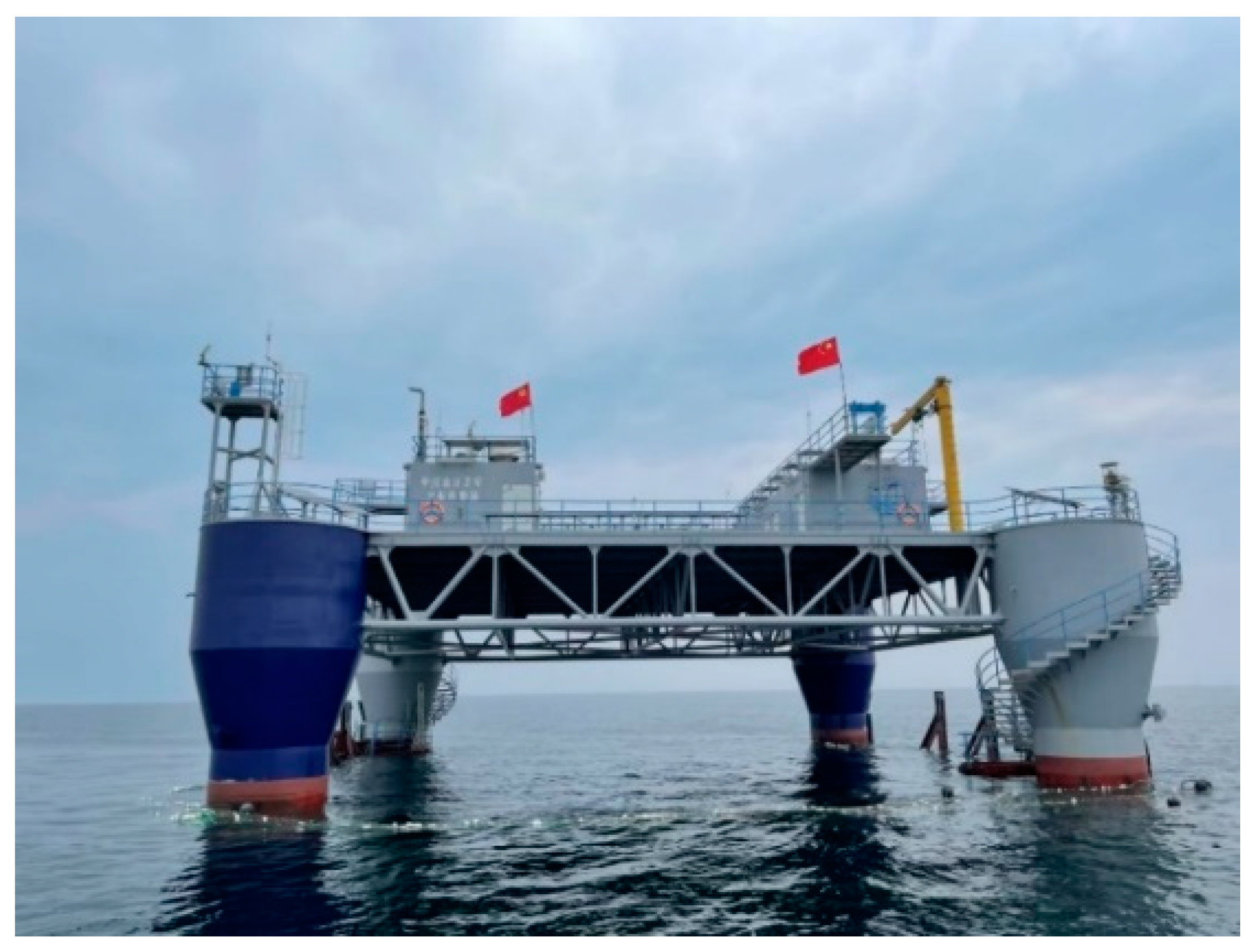
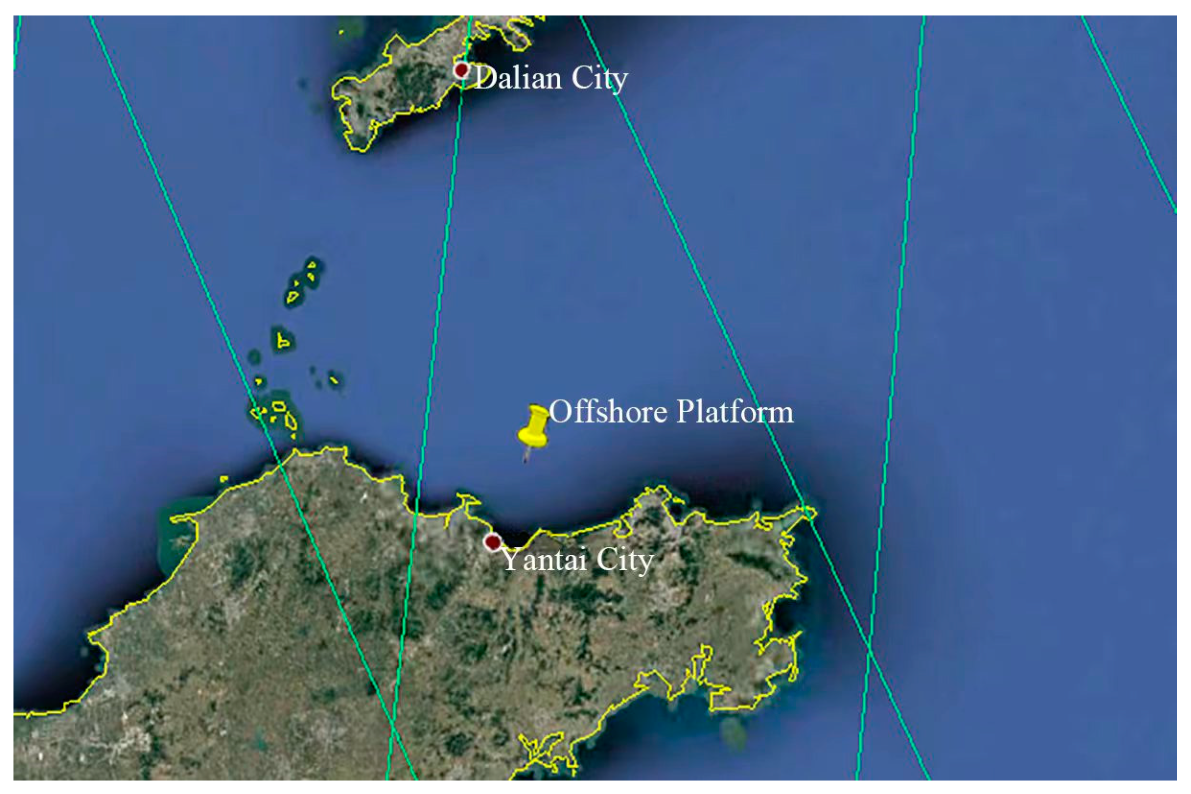
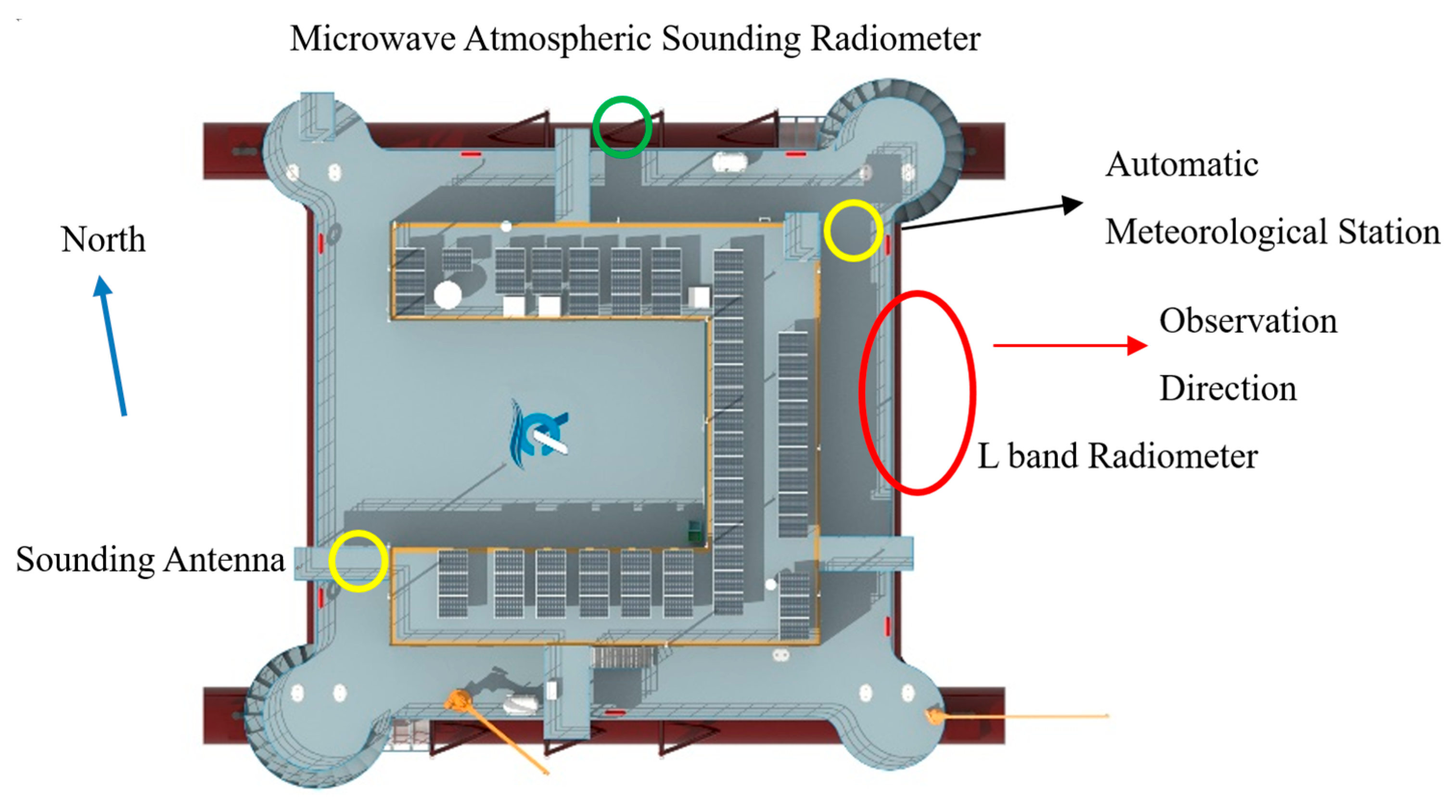
2.1. Offshore Observation Experiment

The 1.4~1.427 GHz frequency band has been accepted internationally for retrieving SSS [20], and the sea surface brightness temperature in this band is highly sensitive to SSS and can realize all-time and all-weather observation. This frequency band is also protected by international treaties and generally does not experience interference from human signals.

An experimental study was conducted on an offshore platform (as shown in Figure 1) from 11 August 2022 to 1 September 2022, with the observation platform situated about 30 km north of Yangma Island in Yantai, China (121.622°E, 37.695°N, as shown in Figure 2).

In the experiment, the sea surface brightness temperature was measured at different incident angles through a radiometer; the SST and SSS were synchronously obtained through the CTD (conductivity, temperature, and depth); the atmospheric pressure, atmospheric temperature, atmospheric relative humidity, wind speed, and wind direction were synchronously obtained through the automatic meteorological station. The primary technical indicators of the equipment are shown in

Table 1. Primary technical indicators of the radiometer.

Parameter	Indicator
Frequency Band	L
Central Frequency	1.415 GHz
3 dB Bandwidth	10 MHz
Polarization	H/V
Spatial Resolution	≤20°
Sensitivity	≤0.1 K@1 s Integration Time

,

Table 2. Primary technical indicators of the CTD.

Parameter	Measurement Range	Accuracy
Temperature	0~35 °C	0.002 °C
Conductivity	0~7 S/m	0.0003 S/m

and

Table 3. Primary technical indicators of the automatic meteorological station.

Parameter	Measurement Range	Accuracy
Atmospheric Pressure (hPa)	850~1050	±1
Atmospheric Temperature (°C)	−50~50	±0.3
Atmospheric Relative Humidity (%)	0~100	±3
Wind Speed (m/s)	0~70	±1
Wind Direction (°)	0~360	±10

.

To reduce the impact of the sun and RFI, the entire observing process was conducted with our backs to the sun and not towards the land, and the installation diagram of observation platform equipment is as follows (Figure 3):

2.2. Sea Salinity Data Processing

In the experiment, the CTD directly measures the conductivity of seawater, and it needs to be converted into seawater salinity using the following equation (2 psu ≤ S ≤ 42 psu, −2 °C ≤ T ≤ 35 °C) [21,22].

$$S={\displaystyle \sum _{i=0}^5{a}_i{R}_T^{i/2}}+\frac{T-15}{1+0.0162\left(T-15\right)}{\displaystyle \sum _{i=0}^5{b}_i{R}_T^{i/2}}$$

(1)

where T (°C) is the temperature of seawater, R_T is the ratio of the conductivity at a standard atmospheric pressure and a temperature of T (the superscript represents atmospheric pressure), and the coefficients of Equation (1) are shown in

Table 4. Coefficients of Equation (1).

Coefficient	Value	Coefficient	Value
a0	0.008	b0	0.0005
a1	−0.1692	b1	−0.0056
a2	25.3851	b2	−0.0066
a3	14.0941	b3	−0.0375
a4	−7.0261	b4	0.0636
a5	2.7081	b5	−0.0144
sum	35	sum	0

.

2.3. Wind Speed Data Processing

The wind speed data used in SSS inversion is generally the wind speed at a 10 m altitude; however, the installation height of the automatic meteorological station cannot fully meet this requirement. Therefore, the following equation needs to be used to convert the measured wind speed data into the wind speed at a 10 m altitude.

$$U_z=\frac{U_{\ast }}{0.4}\left(\ln \frac{z}{\frac{6.84\times {10}^{-5}}{U_{\ast }}+4.28\times {10}^{-3}{U}_{\ast }^2-4.43\times {10}^{-4}}\right)$$

(2)

where U_z (m/s) is the wind speed at z (m) altitude, and U_* is the wind friction velocity.

2.4. Removing the Effects of Atmospheric Radiation and Cosmic Radiation

Figure 4 depicts the complete transmission process of sea surface radiation to the offshore platform radiometer.

The sea surface brightness temperature that the offshore platform radiometer received was influenced by SSR, sea surface foam, the atmosphere, and cosmic radiation [23,24]. After removing all RFI-contaminated data and the data with large fluctuations, the brightness temperature data that the radiometer measured can be expressed as follows [25,26]:

$$T_{Bp\_MR}=T_{Bp\_SSR+Foam}+\left(1-e_{p\_SSR+Foam}\right)\cdot \left(T_{BD}+\Gamma T_{B\_COS}\right)$$

(3)

where T_{Bp_MR} is the p polarization brightness temperature received by the radiometer (p = H, V that stand for the horizontal polarization and vertical polarization of electromagnetic waves, respectively), T_{Bp_SSR+Foam} and e_{p_SSR+Foam} are the p polarization sea surface brightness temperature and the p polarization sea surface emissivity under the impact of SSR and sea surface foam, respectively, T_BD is the atmospheric downward radiation, Γ is the atmospheric transmittance, and T_{B_COS} = 3.7 K [27] is the cosmic radiation brightness temperature (there are also some papers that take T_{B_COS} = 2.73 K [26,28,29], and this article will explain the reason for not taking this value in subsequent sections). The equations for removing the effects of atmospheric radiation and cosmic radiation are as follows [30]:

$$T_{Bp\_SSR+Foam}=\frac{T_{Bp\_MR}-\left(T_{BD}+\Gamma T_{B\_\cos }\right)}{SST-\left(T_{BD}+\Gamma T_{B\_\cos }\right)}\cdot SST$$

(4)

$$T_{BD}=\sec \theta {\displaystyle {\int }_0^{\infty }\left[k_{O_2}\left(z\right)+k_{H_{2}O}\left(z\right)\right]\cdot T_a\left(z\right)\exp \left(-\tau \sec \theta \right)\mathrm{d}z}$$

(5)

$$\Gamma =\exp \left[-\sec \theta \cdot \tau \right]$$

(6)

$$\tau ={\displaystyle {\int }_0^h\left[k_{O_2}\left(z\right)+k_{H_{2}O}\left(z\right)\right]\mathrm{d}z}$$

(7)

$$k_{O_2}\left(z,f\right)=1.1\times {10}^{-2}{f}^2\left[\frac{P_a\left(z\right)}{1013}\right]\cdot {\left[\frac{300}{T_a\left(z\right)}\right]}^2\cdot \gamma \left[\frac{1}{{\left(f-f_0\right)}^2+{\gamma }^2}+\frac{1}{f^2+{\gamma }^2}\right]$$

(8)

$$\gamma ={\gamma }_0\left(\frac{P_a}{1013}\right){\left(\frac{300}{T_a}\right)}^{0.85}$$

(9)

$${\gamma }_0=\{\begin{array}{c}0.59,P_a\ge 333\\ 0.59\cdot \left[1+0.0031\cdot \left(333-P_a\right)\right],25\le P_a<333\\ 1.18,P_a\le 25\end{array}$$

(10)

$$k_{H_{2}O}\left(z,f\right)=k\left(f,22\right)+k_r\left(f\right)$$

(11)

$$k\left(f,22\right)=2f^2{\rho }_v\left(z\right){\left(\frac{300}{T_a\left(z\right)}\right)}^{2.5}\exp \left(-\frac{644}{T_a\left(z\right)}\right)\cdot \left[\frac{{\gamma }_1}{{\left(494.4-f^2\right)}^2+4f^2{\gamma }_1^2}\right]$$

(12)

$$k_r\left(f\right)=2.4\times {10}^{-6}{f}^2{\rho }_v\left(z\right){\left(\frac{300}{T_a\left(z\right)}\right)}^{1.5}{\gamma }_1$$

(13)

$${\gamma }_1=2.85\left[\frac{P_a\left(z\right)}{1013}\right]\cdot {\left[\frac{300}{T_a\left(z\right)}\right]}^{0.626}\cdot \left(1+0.018\frac{{\rho }_v\left(z\right)T_a\left(z\right)}{P_a\left(z\right)}\right)$$

(14)

$$T_a\left(z\right)=\{\begin{array}{c}{T}_0-6.5z,0\le z\le 11\\ T_a\left(11\right),11\le z\le 20\\ T_a\left(11\right)+\left(z-20\right),20\le z\le 32\end{array}$$

(15)

$$P_a\left(z\right)=P_0\cdot \exp \left(-\frac{z}{7.7}\right)$$

(16)

$${\rho }_v\left(z\right)={\rho }_0\exp \left(-\frac{z}{CH}\right)$$

(17)

where SST is the sea surface temperature in Kelvin, θ is the incident angle of the radiometer, k_a(z) is the atmospheric attenuation coefficient (a can be taken as O₂ and H₂O, representing oxygen and water vapor, respectively), z is the altitude in kilometers, τ is atmospheric optical depth, h is the upper boundary of the atmosphere (for most microwave remote sensing of the Earth, and certainly at the L-band, it is only the lower 30 km of the atmosphere that needs to be taken into consideration), f is the frequency of the radiometer (1.415 GHz), f₀ is the absorption line frequency (60 GHz), γ (GHz) is the line width parameter, γ₀ is the nonresonant line width, k(f, 22) is the absorption coefficient for the 22.235 GHz spectral line, k_r(f) is the residual absorption coefficient, γ₁ (GHz) is the line width parameter, T_a(z), P_a(z), and ρ_v(z) are the temperature profile, the pressure profile, and the water vapor density profile, respectively, T₀ is the atmospheric temperature in Kelvin at sea level, T_a(11) is the atmospheric temperature in Kelvin at z = 11 km, P₀ is the atmospheric pressure in millibars at sea level, ρ₀ is the water vapor density in g/m³ at sea level, and CH is the scale height, which is typically chosen to be between 2 and 2.5 km (in this article, CH = 2.25 km was taken).

2.5. Removing the Effects of Sea Surface Foam and Flat Sea Surface Brightness Temperature

After removing the effects of atmospheric radiation and cosmic radiation from the brightness temperature data received by the radiometer, the processed data can be expressed as follows [31,32]:

$$\begin{array}{ll}{T}_{Bp\_SSR+Foam}& =T_{Bp\_Sur}\cdot \left(1-F_r\right)+F_r\cdot T_{Bp\_Foam}\\ & =\left(T_{Bp\_Flat}+\Delta T_{Bp\_SSR}\right)\cdot \left(1-F_r\right)+F_r\cdot T_{Bp\_Foam}\end{array}$$

(18)

where T_{Bp_Sur} is the p polarization sea surface brightness temperature under the impact of SSR, F_r is the whitecap coverage rate, T_{Bp_Foam} is the p polarization brightness temperatures of the foam-covered sea surface, T_{Bp_Flat} is the p polarization flat sea surface brightness temperature, and ΔT_{Bp_SSR} is the p polarization brightness temperature increment generated by the SSR. The equation for removing the effects of sea surface foam and flat sea surface brightness temperature is as follows:

$$\Delta T_{Bp\_SSR}=\frac{T_{Bp\_SSR+Foam}-F_r\cdot T_{Bp\_Foam}}{1-F_r}-T_{Bp\_Flat}$$

(19)

F_r can be calculated using the following equation [33]:

$$F_r=1.95\times {10}^{-5}{U}_{10}^{2.55}\exp \left(0.0861\Delta T\right)$$

(20)

where U₁₀ is the wind speed at a 10 m altitude, and ΔT = SST − T₀ is the sea air temperature difference.

T_{Bp_Foam} can be calculated using the following equations [34]:

$$T_{BH\_Foam}=\left(208+1.29f\right)\cdot \left(1-1.748\times {10}^{-3}\theta -7.336\times {10}^{-5}{\theta }^2+1.044\times {10}^{-7}{\theta }^3\right)$$

(21)

$$\begin{array}{l}{T}_{BV\_Foam}=\left(208+1.29f\right)\cdot \\ \left(1-9.946\times {10}^{-4}\theta +3.218\times {10}^{-5}{\theta }^2-1.187\times {10}^{-6}{\theta }^3+7\times {10}^{-20}{\theta }^{10}\right)\end{array}$$

(22)

where f is the frequency of the radiometer, and θ is the incident angle of the radiometer.

T_{Bp_Flat} can be calculated using the following equations [35,36,37]:

$$T_{Bp\_Flat}=\left(1-r_{p\_Flat}\right)\cdot SST$$

(23)

$$r_{H\_Flat}={\left|\frac{\cos \theta -\sqrt{{\epsilon }_r-{\left(\frac{n}{n^{\prime }}\right)}^2{\sin }^2\theta }}{\cos \theta +\sqrt{{\epsilon }_r-{\left(\frac{n}{n^{\prime }}\right)}^2{\sin }^2\theta }}\right|}^2$$

(24)

$$r_{V\_Flat}={\left|\frac{{\epsilon }_r\cos \theta -\sqrt{{\epsilon }_r-{\left(\frac{n}{n^{\prime }}\right)}^2{\sin }^2\theta }}{{\epsilon }_r\cos \theta +\sqrt{{\epsilon }_r-{\left(\frac{n}{n^{\prime }}\right)}^2{\sin }^2\theta }}\right|}^2$$

(25)

where r_{p_Flat} is the p polarization flat sea surface reflectivity, θ is the incident angle of the radiometer, n = n′ − jn″ is the complex refractive index of seawater, and ε_r is the relative permittivity of seawater and can be described with the relaxation theory equation, such as the Cole–Cole equation [38] and the double debye equation [39], as shown below:

$${\epsilon }_r={\epsilon }_{\infty }+\frac{{\epsilon }_s-{\epsilon }_{\infty }}{1+{\left(j\omega \tau \right)}^{1-\alpha }}-j\frac{\sigma }{\omega {\epsilon }_0}$$

(26)

$$\begin{array}{cc}\hfill {\epsilon }_r& ={\epsilon }_{\infty }+\frac{{\epsilon }_s-{\epsilon }_1}{1+j\omega {\tau }_1}+\frac{{\epsilon }_1-{\epsilon }_{\infty }}{1+j\omega {\tau }_2}-j\frac{\sigma }{\omega {\epsilon }_0}\hfill \\ & ={\epsilon }_{\infty }+\frac{{\epsilon }_s-{\epsilon }_1}{1+j\frac{f}{f_1}}+\frac{{\epsilon }_1-{\epsilon }_{\infty }}{1+j\frac{f}{f_2}}-j\frac{\sigma }{\omega {\epsilon }_0}\hfill \end{array}$$

(27)

where ε_∞ is the relative permittivity at an infinite frequency, ε_s is the static relative permittivity, j is an imaginary unit, ω = 2πf is the radian frequency with f in hertz, τ is the relaxation time in seconds, α is an empirical parameter that represents the distribution of relaxation times, σ is the ionic conductivity in mhos/meter, ε₀ ≈ 8.85419 × 10⁻¹² is the permittivity of free space in farads/meters, ε₁ is the relative permittivity at an intermediate frequency, τ₁ and τ₂ are the first and second debye relaxation times in seconds, and f₁ and f₂ are the first and second debye relaxation frequencies in hertz.

The parameters of the Cole–Cole equation and the double debye equation can be expressed as a function of SST(T) and SSS(S) with the L-band relative permittivity model, such as KS (1977) [40], ModKS (2000) [41], BA (2003) [42], BA (2004) [43], GW (2017) [44], and GW (2021) [45] can all be used to depict the parameters in the Cole–Cole equation, and MW (2004) [46], FASTEM (2011) [47], and MW (2012) [48] can all be used to depict the parameters in the double debye equation. By way of illustration, the MW (2004) depicts the parameters in the double debye equation as the following functions of T and S:

$${\epsilon }_s\left(T,S\right)={\epsilon }_s\left(T,0\right)\cdot \exp \left[b_{0}S+b_1{S}^2+b_{2}TS\right]$$

(28)

$${\epsilon }_s\left(T,0\right)=\frac{3.70886\times {10}^4-8.2168\times {10}^{1}T}{4.21854\times {10}^2+T}$$

(29)

$$f_1\left(T,S\right)=f_1\left(T,0\right)\cdot \left[1+S\cdot \left(b_3+b_{4}T+b_5{T}^2\right)\right]$$

(30)

$$f_1\left(T,0\right)=\frac{45+T}{a_3+a_{4}T+a_5{T}^2}$$

(31)

$${\epsilon }_1\left(T,S\right)={\epsilon }_1\left(T,0\right)\cdot \exp \left[b_{6}S+b_7{S}^2+b_{8}TS\right]$$

(32)

$${\epsilon }_1\left(T,0\right)=a_0+a_{1}T+a_2{T}^2$$

(33)

$$f_2\left(T,S\right)=f_2\left(T,0\right)\cdot \left[1+S\cdot \left(b_9+b_{10}T\right)\right]$$

(34)

$$f_2\left(T,0\right)=\frac{45+T}{a_8+a_{9}T+a_{10}{T}^2}$$

(35)

$${\epsilon }_{\infty }\left(T,S\right)={\epsilon }_{\infty }\left(T,0\right)\cdot \left[1+S\cdot \left(b_{11}+b_{12}T\right)\right]$$

(36)

$${\epsilon }_{\infty }\left(T,0\right)=a_6+a_{7}T$$

(37)

$$\sigma \left(T,S\right)=\sigma \left(T,35\right)\cdot R_{15}\left(S\right)\cdot \frac{R_T\left(S\right)}{R_{15}\left(S\right)}$$

(38)

$$\begin{array}{c}\sigma \left(T,35\right)=2.903602+8.607\times {10}^{-2}T\\ +4.738817\times {10}^{-4}{T}^2-2.991\times {10}^{-6}{T}^3+4.3047\times {10}^{-9}{T}^4\end{array}$$

(39)

$$R_{15}\left(S\right)=S\cdot \frac{37.5109+5.45216S+1.4409\times {10}^{-2}{S}^2}{1004.75+182.283S+S^2}$$

(40)

$$\frac{R_T\left(S\right)}{R_{15}\left(S\right)}=1+\frac{{\alpha }_0\left(T-15\right)}{\left({\alpha }_1+T\right)}$$

(41)

$${\alpha }_0=\frac{6.9431+3.2841S-9.9486\times {10}^{-2}{S}^2}{84.850+69.024S+S^2}$$

(42)

$${\alpha }_1=49.843-0.2276S+0.198\times {10}^{-2}{S}^2$$

(43)

$${\epsilon }_0=\frac{1}{1.7975\cdot 2\pi }\times {10}^{-10}$$

(44)

The coefficients of Equations (28)–(44) are shown in

Table 5. Coefficients of Equations (28)–(44).

Coefficient	Value	Coefficient	Value
a0	5.7230	b0	−3.56417 × 10−3
a1	2.2379 × 10−2	b1	4.74868 × 10−6
a2	−7.1237 × 10−4	b2	1.15574 × 10−5
a3	5.0478	b3	2.39357 × 10−3
a4	−7.0315 × 10−2	b4	−3.13530 × 10−5
a5	6.0059 × 10−4	b5	2.52477 × 10−7
a6	3.6143	b6	−6.28908 × 10−3
a7	2.8841 × 10−2	b7	1.76032 × 10−4
a8	1.3652 × 10−1	b8	−9.22144 × 10−5
a9	1.4825 × 10−3	b9	−1.99723 × 10−2
a10	2.4166 × 10−4	b10	1.81176 × 10−4
		b11	−2.04265 × 10−3
		b12	1.57883 × 10−4

.

The equations of other relative permittivity models will not be listed in this article. Finally, 18 sets of SSR brightness temperature increment data (including 9 sets of H-polarization data and 9 sets of V-polarization data) were generated by using the aforementioned nine relative permittivity models to process the data.

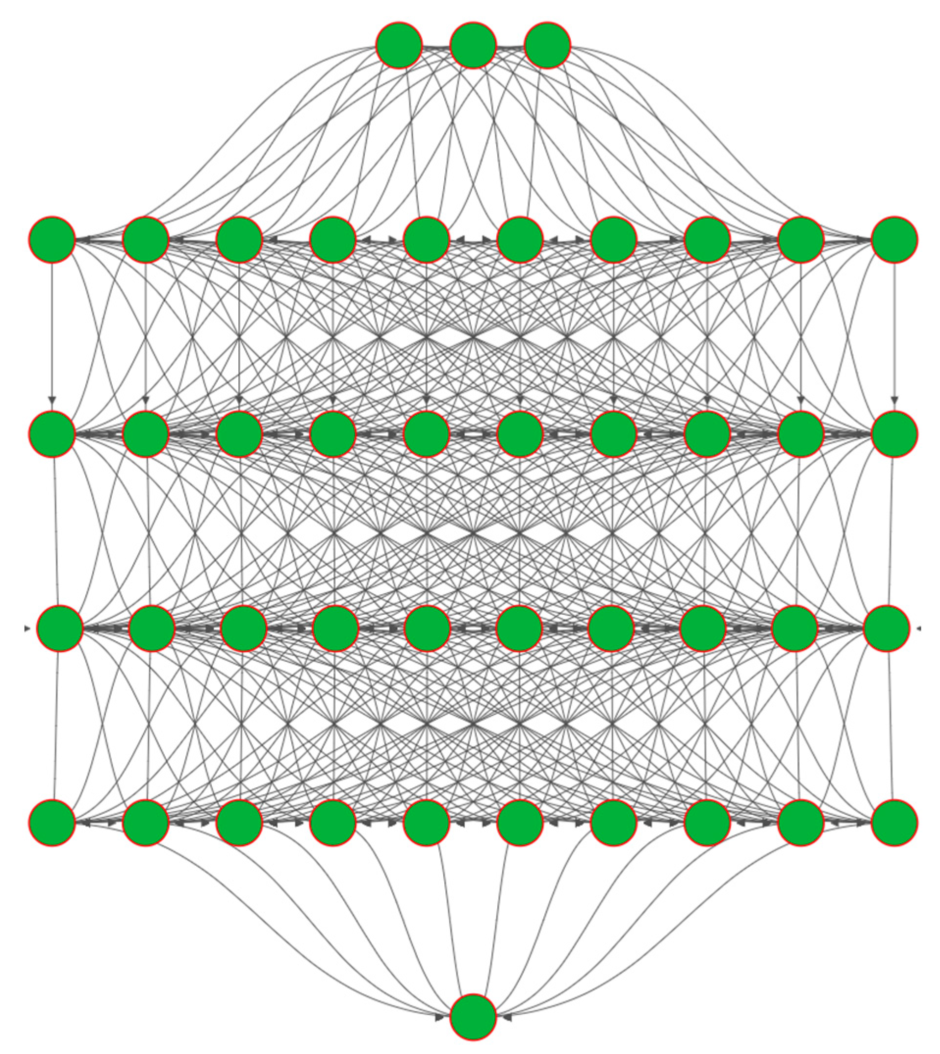
3. Deep Neural Network Model

The universal approximation theorem [49,50] shows that a feedforward neural network with a linear output layer and at least one hidden layer with any kind of “squeeze” property activation function can approximate any Borel measurable function from one finite dimensional space to another with any precision as long as enough neurons are given to its hidden layer. Therefore, the feedforward neural network was chosen in this paper.

The research ranges of θ, U₁₀, and WD (wind direction) in 18 sets of SSR brightness temperature increment data were set to [0°, 60°], [0, 12 m/s], and [0, 360°], respectively, and 18 datasets, which correspond to 9 H-polarization DNN models and 9 V-polarization DNN models, were uniformly and randomly selected from the research ranges, and each dataset contains 35,000 sets of data in the form of [θ, U₁₀, WD, ΔT_{Bp_SSR}]; then, each dataset was randomly divided into a training set and a testing set in an 8:2 ratio.

Before DNN training, training sets and test sets should be normalized. The data normalization process is to convert all data into data between 0 and 1, which is to eliminate the order of magnitude difference of data of various dimensions and avoid large network prediction errors caused by a large order of magnitude difference in input data. The data normalization method in this paper is the max–min method [51].

$$x_k=\frac{\left(x_k-x_{\min }\right)}{\left(x_{\max }-x_{\min }\right)}$$

(45)

where x_k is a set of input data, and k is the serial number of a datum. x_max and x_min are the maximum and minimum values of corresponding data.

The output of the DNN model needs to be renormalization to convert to the original range, which is the inverse process of normalization. The equation is as follows:

$$y_k=y_k\cdot \left(y_{\max }-y_{\min }\right)+y_{\min }$$

(46)

where y_k is a set of input data, and k is the serial number of a datum. y_max and y_min are the maximum and minimum values of corresponding data of the training sets.

The training model in this paper is a six-layer DNN model, with the input layer having three neurons for θ, U₁₀, and WD, the output layer having one neuron for ΔT_{Bp_SSR}, and the hidden layer having 100 neurons; the random initial values were used as the DNN parameters, and the fundamental architecture of the DNN model is as follows (Figure 5):

The PReLU [52] was used as the activation function, as shown below (Figure 6):

$$\mathrm{PReLU}\left(x\right)=\{\begin{array}{c}x,\mathrm{if}x>0\\ \alpha x,\mathrm{if}x\le 0\end{array}$$

(47)

The learnable parameter α, which is updated continually throughout the training phase, is the slope of the negative semi-axis of PRelu. Additionally, PReLU permits a group of neurons to share an α as well as allowing various neurons to have a distinct α. When α is a very small constant, PReLU can be thought of as LeakyReLU [53], and when α = 0, PReLU becomes ReLU [54].

The MSELoss was used as the loss function of the output layer, as shown below [55]:

$$\mathrm{MSELoss}={\left(\Delta T_{Bp\_SSR\_\mathrm{out}}-\Delta T_{Bp\_SSR\_\mathrm{t}\arg \mathrm{et}}\right)}^2$$

(48)

where ΔT_{Bp_SSR_out} denotes the output value of the output layer neuron and ΔT_{Bp_SSR_target} denotes its target value.

The Adam [56] and Backpropagation algorithms [57,58] were used as the training algorithms, as shown below:

$$u_h=u_{h-1}-\frac{\eta m_h}{\sqrt{v_h+\gamma }}$$

(49)

$$\{\begin{array}{c}{\mathit{W}}^k\left(h+1\right)={\mathit{W}}^k\left(h\right)-\eta {\mathit{\delta }}^k\cdot {\mathit{A}}^{k-1}\\ {\mathit{B}}^k\left(h+1\right)={\mathit{B}}^k\left(h\right)-\eta {\mathit{\delta }}^k\end{array}$$

(50)

where h is the number of iterations, u is the parameter to be optimized, η is the learning rate, m_h is the first-order momentum, v_h is the second-order momentum, γ is a small positive number, W^k is the weight matrix between layers k − 1 and k, δ^k is the error matrix of layer k, A^k is the output matrix of layer k, and B^k is the bias matrix of layer k.

The training process and forecast accuracy of the DNN models are shown in

Table 6. The training process and forecast accuracy of the DNN models.

Model Forecast Accuracy (K)	Learning Rate 0.01 (Iterate 8000 Times)	Learning Rate 0.003 (Iterate 30,000 Times)	Learning Rate 0.001 (Iterate 50,000 Times)	Learning Rate 0.0003 (Iterate 80,000 Times)
KS-H	−0.38~0.47	−0.50~0.24	−0.34~0.25	−0.14~0.29
KS-V	−0.29~0.35	−0.52~0.14	−0.39~0.15	−0.24~0.15
ModKS-H	−0.16~0.69	−0.66~0.12	−0.30~0.21	−0.23~0.12
ModKS-V	−0.26~0.35	−0.44~0.21	−0.23~0.15	−0.17~0.22
BA-H(03)	−0.39~0.47	−0.28~0.38	−0.26~0.12	−0.22~0.06
BA-V(03)	−0.32~0.68	−0.32~0.39	−0.31~0.26	−0.14~0.22
BA-H(04)	−0.38~0.43	−0.63~0.22	−0.37~0.30	−0.29~0.28
BA-V(04)	−0.23~0.76	−0.44~0.40	−0.14~0.38	−0.19~0.23
MW-H(04)	−0.35~0.40	−0.06~0.77	−0.63~0.03	−0.31~0.36
MW-V(04)	−0.45~0.75	−0.56~0.59	−0.19~0.31	−0.14~0.25
FASTEM-H	−0.42~0.48	−0.40~0.17	−0.31~0.11	−0.28~0.18
FASTEM-V	−0.20~0.73	−0.79~0.40	−0.51~0.35	−0.27~0.28
MW-H(12)	−0.83~0.45	−0.63~0.55	−0.41~0.62	−0.23~0.36
MW-V(12)	−0.41~0.48	−0.36~0.27	−0.27~0.21	−0.17~0.27
GW-H(17)	−0.49~0.77	−0.24~0.52	−0.27~0.37	−0.12~0.37
GW-V(17)	−0.55~0.52	−0.72~0.29	−0.18~0.23	−0.13~0.22
GW-H(21)	−0.49~0.46	−0.78~0.32	−0.64~0.31	−0.13~0.22
GW-V(21)	−0.23~0.41	−0.59~0.22	−0.22~0.14	−0.24~0.13

.

The forecast accuracy of the DNN models can be further improved by further lowering the learning rate and continuing training, and the final performance of the DNN models is shown in

Table 7. Final performance of the DNN models.

DNN Model	Forecast Accuracy (K)	RMSE	MAE
KS-H	−0.13~0.14	0.0157	0.0103
KS-V	−0.11~0.13	0.0156	0.0090
ModKS-H	−0.13~0.13	0.0161	0.0101
ModKS-V	−0.13~0.16	0.0185	0.0114
BA-H(03)	−0.14~0.16	0.0177	0.0108
BA-V(03)	−0.15~0.16	0.0191	0.0118
BA-H(04)	−0.17~0.13	0.0183	0.0121
BA-V(04)	−0.15~0.15	0.0173	0.0109
MW-H(04)	−0.15~0.17	0.0182	0.0124
MW-V(04)	−0.15~0.13	0.0168	0.0106
FASTEM-H	−0.14~0.15	0.0169	0.0106
FASTEM-V	−0.14~0.17	0.0176	0.0102
MW-H(12)	−0.17~0.16	0.0189	0.0113
MW-V(12)	−0.17~0.16	0.0190	0.0110
GW-H(17)	−0.15~0.15	0.0177	0.0107
GW-V(17)	−0.14~0.17	0.0166	0.0095
GW-H(21)	−0.13~0.17	0.0170	0.0100
GW-V(21)	−0.17~0.13	0.0184	0.0105

.

Where RMSE and MAE are the Root Mean Square Error and the Mean Absolute Error [59,60], and their calculation equations are as follows:

$$RMSE=\sqrt{\frac{{\displaystyle \sum _{i=1}^n{x}_i^2}}{n}}=\sqrt{\frac{x_1^2+x_2^2+\cdots +x_n^2}{n}}$$

(51)

$$MAE=\frac{{\displaystyle \sum _{i=1}^n\left|x_i\right|}}{n}=\frac{\left|x_1\right|+\left|x_2\right|+\cdots +\left|x_n\right|}{n}$$

(52)

This article chooses SSR brightness temperature increment models like Hollinger [9], WISE (2003) [10], WISE (2004) (containing two models calculated with the incident angle and wind speed, which are called WISE1 and WISE2, respectively, according to the order in reference [11]), TSM [16], and SSA [17] for research based on the data characteristics of offshore platform experiments, and 108 forward models (including 54 H-polarization models and 54 V-polarization models) can be obtained by combining each SSR brightness temperature increment model with the aforementioned 9 relative permittivity models. The test sets were substituted into the 108 forward models, and the accuracy is shown in

Table 8. Performance of the forward models on the test sets.

Model Forecast Accuracy (K)	Hollinger	WISE	WISE1	WISE2	TSM	SSA
KS-H	−1.57~1.49	−1.55~1.71	−1.51~1.69	−1.65~1.54	−0.47~0.61	−0.60~0.81
KS-V	−0.79~1.29	−0.79~1.11	−0.79~1.18	−0.81~0.98	−0.35~0.55	−0.48~0.69
ModKS-H	−2.38~0.59	−2.35~0.80	−2.32~0.79	−2.46~0.63	−1.28~−0.26	−1.41~−0.05
ModKS-V	−1.80~0.11	−1.80~−0.07	−1.80~−0.01	−1.82~−0.20	−1.33~−0.58	−1.47~−0.49
BA(03)-H	−2.04~0.59	−2.02~0.80	−1.98~0.79	−2.12~0.63	−0.94~−0.50	−1.07~−0.32
BA(03)-V	−4.03~−1.14	−4.20~−1.33	−4.12~−1.26	−4.36~−1.45	−3.89~−1.94	−3.51~−1.75
BA(04)-H	−0.31~2.55	−0.29~2.77	−0.25~2.76	−0.39~2.60	0.79~1.46	0.66~1.65
BA(04)-V	−1.37~1.41	−1.53~1.23	−1.47~1.29	−1.69~1.10	−1.23~0.61	−0.85~0.81
MW(04)-H	−1.25~1.48	−1.23~1.70	−1.19~1.69	−1.33~1.53	−0.15~0.41	−0.28~0.59
MW(04)-V	−2.82~−0.02	−2.98~−0.20	−2.91~−0.13	−3.14~−0.33	−2.67~−0.81	−2.30~−0.62
FASTEM-H	−1.34~1.38	−1.32~1.60	−1.28~1.59	−1.42~1.43	−0.24~0.30	−0.37~0.48
FASTEM-V	−2.98~−0.17	−3.15~−0.35	−3.07~−0.28	−3.30~−0.48	−2.84~−0.97	−2.46~−0.77
MW(12)-H	−1.25~1.48	−1.23~1.70	−1.19~1.69	−1.33~1.53	−0.15~0.41	−0.28~0.59
MW(12)-V	−2.82~−0.02	−2.98~−0.20	−2.91~−0.13	−3.14~−0.33	−2.67~−0.81	−2.30~−0.62
GW(17)-H	−1.55~1.50	−1.52~1.72	−1.49~1.70	−1.63~1.55	−0.45~0.62	−0.58~0.81
GW(17)-V	−0.82~1.59	−0.82~1.41	−0.82~1.48	−0.84~1.28	−0.34~0.79	−0.51~0.99
GW(21)-H	−1.58~1.48	−1.56~1.69	−1.52~1.68	−1.66~1.52	−0.48~0.60	−0.61~0.80
GW(21)-V	−0.80~1.28	−0.80~1.09	−0.80~1.16	−0.82~0.97	−0.36~0.53	−0.49~0.67

.

The RMSE and MAE of the 108 forward models and the 18 DNN models on the test sets are shown in Figure 7, Figure 8, Figure 9 and Figure 10.

It can be seen from Table 7 and Table 8, and Figure 7, Figure 8, Figure 9 and Figure 10, that the DNN models perform significantly better than the existing models, and that their calculation accuracy is close to the detection accuracy of the radiometer (0.1 K).

Furthermore, this study processed offshore experiment data using T_{B_COS} = 2.73 K and employed the same methodology for its research and analysis, and the findings demonstrate that although the 18 DNN models can also be trained to the level of Table 7, the errors of the 108 forward models in Table 8 will increase. As a result, the experimental data in this article were processed with T_{B_COS} = 3.7 K (the processed results of T_{B_COS} = 2.73 K will not be listed in this article).

4. Discussion

The forecast accuracy of the DNN models should be set above 0.1 K because the detection accuracy of the radiometer utilized in the offshore observation experiment is 0.1 K. Excessive training (such as setting the forecast accuracy within 0.1 K) will make the DNN models learn too much error from the radiometer itself, which will lower the reliability of the prediction results of the DNN models. As a result, the threshold for ending training regarding the DNN models in this paper is set to 0.1~0.2 K, and Table 7 shows that all DNN models met the standards.

The reason for the low forecast accuracy of Hollinger, WISE, WISE1, and WISE2 is that they do not consider the influence of wind direction. Although the forecast accuracy of TSM and SSA is relatively high, they are unable to match the detection accuracy of the radiometer (0.1 K), which may be due to the error of the ocean wave spectrum of the offshore area used by the two algorithms.

The relative permittivity model also has an impact on the forward model. It can be seen from Table 8 that KS (1977), MW (2004), FASTEM (2011), MW (2012), GW (2017), and GW (2021) have good performances for the H-polarization forward models; KS (1977), GW (2017), and GW (2021) have good performances for the V-polarization forward models; and KS (1977) and GW (2021) perform similarly and well on the two polarization forward models.

5. Conclusions

The calculation results of different forward models, which are composed of different relative permittivity models and SSR brightness temperature increment models, are different, and the impact of this calculation difference exceeds the accuracy requirement of the SSS inversion. The existing SSR brightness temperature increment models, which primarily include empirical models and theoretical models, cannot match all the relative permittivity models, and can only obtain good results under the specific relative permittivity model, while the errors under other relative permittivity models are large. Therefore, different SSR brightness temperature increment models should be provided for different relative permittivity models to make the calculation results of the forward model as close to the actual sea surface situation as possible. In order to address this problem, this paper proposes a universal DNN model architecture and corresponding training scheme, and provides 18 different SSR brightness temperature increment models (including 9 H-polarization models and 9 V-polarization models) for 9 widely used L-band relative permittivity models utilizing DNN based on the offshore experiment data, and compares them with the existing models. The results show that the DNN models perform significantly better than the existing models, and that their forecast accuracy is close to the detection accuracy of the radiometer (0.1 K). Therefore, this study effectively solves the problem of SSR brightness temperature correction under different relative permittivity models, and provides a theoretical support for high-precision SSS inversion research.

References

1. Ouyang, Y.; Zhang, Y.; Chi, J.; Sun, Q.; Du, Y. Deviations of satellite-measured sea surface salinity caused by environmental factors and their regional dependence. Remote Sens. Environ. 2023, 285, 113411. [Google Scholar] [CrossRef]
2. Zhang, L.; Zhang, Y.; Yin, X. Aquarius sea surface salinity retrieval in coastal regions based on deep neural networks. Remote Sens. Environ. 2023, 284, 113357. [Google Scholar] [CrossRef]
3. Jang, E.; Kim, Y.J.; Im, J.; Park, Y.-G.; Sung, T. Global sea surface salinity via the synergistic use of SMAP satellite and HYCOM data based on machine learning. Remote Sens. Environ. 2022, 273, 112980. [Google Scholar] [CrossRef]
4. Akins, A.; Brown, S.; Lee, T.; Misra, S.; Yueh, S. Simulation Framework and Case Studies for the Design of Sea Surface Salinity Remote Sensing Missions. IEEE J. Sel. Top. Appl. Earth Obs. Remote Sens. 2023, 16, 1321–1334. [Google Scholar] [CrossRef]
5. Fournier, S.; Bingham, F.M.; González-Haro, C.; Hayashi, A.; Ulfsax Carlin, K.M.; Brodnitz, S.K.; González-Gambau, V.; Kuusela, M. Quantification of Aquarius, SMAP, SMOS and Argo-Based Gridded Sea Surface Salinity Product Sampling Errors. Remote Sens. 2023, 15, 422. [Google Scholar] [CrossRef]
6. Gabarró Prats, C. Study of Salinity Retrieval Errors for the SMOS Mission. Ph.D. Thesis, Universitat Politècnica de Catalunya, Barcelona, Spain, 2004. [Google Scholar]
7. Camps, A.; Duffo, N.; Vall-Llossera, M.; Vallespin, B. Sea surface salinity retrieval using multi-angular L-band radiometry: Numerical study using the SMOS End-to-end Performance Simulator. In Proceedings of the IEEE International Geoscience and Remote Sensing Symposium, Toronto, ON, Canada, 24–28 June 2002. [Google Scholar] [CrossRef]
8. Dinnat, E.P.; Boutin, J.; Yin, X.; Le Vine, D.M. Inter-comparison of SMOS and aquarius Sea Surface Salinity: Effects of the dielectric constant and vicarious calibration. In Proceedings of the 2014 13th Specialist Meeting on Microwave Radiometry and Remote Sensing of the Environment (MicroRad), Pasadena, CA, USA, 24–27 March 2014; pp. 55–60. [Google Scholar] [CrossRef]
9. Hollinger, J.P. Passive Microwave Measurements of Sea Surface Roughness. IEEE Trans. Geosci. Electron. 1971, 9, 165–169. [Google Scholar] [CrossRef]
10. Gabarró, C.; Vall-Llossera, M.; Font, J.; Camps, A. Determination of sea surface salinity and wind speed by L-band microwave radiometry from a fixed platform. Int. J. Remote Sens. 2004, 25, 111–128. [Google Scholar] [CrossRef]
11. Camps, A.; Font, J.; Vall-Llossera, M.; Gabarro, C.; Corbella, I.; Duffo, N.; Torres, F.; Blanch, S.; Aguasca, A.; Villarino, R.; et al. The WISE 2000 and 2001 field experiments in support of the SMOS mission: Sea surface L-band brightness temperature observations and their application to sea surface salinity retrieval. IEEE Trans. Geosci. Remote Sens. 2004, 42, 804–823. [Google Scholar] [CrossRef]
12. Gabarró, C.; Font, J.; Camps, A.; Vall-Llossera, M.; Julià, A. A new empirical model of sea surface microwave emissivity for salinity remote sensing. Geophys. Res. Lett. 2004, 31, 113. [Google Scholar] [CrossRef]
13. Yueh, S.H.; Tang, W.; Fore, A.G.; Neumann, G.; Hayashi, A.; Freedman, A.; Chaubell, J.; Lagerloef, G.S.E. L-Band Passive and Active Microwave Geophysical Model Functions of Ocean Surface Winds and Applications to Aquarius Retrieval. IEEE Trans. Geosci. Remote Sens. 2013, 51, 4619–4632. [Google Scholar] [CrossRef]
14. Stogryn, A. The apparent temperature of the sea at microwave frequencies. IEEE Trans. Antennas Propag. 1967, 15, 278–286. [Google Scholar] [CrossRef]
15. Soto-Crespo, J.M.; Friberg, A.T.; Nieto-Vesperinas, M. Scattering from slightly rough random surfaces: A detailed study on the validity of the small perturbation method. J. Opt. Soc. Am. A 1990, 7, 1185–1201. [Google Scholar] [CrossRef]
16. Ma, W.; Du, Y.; Liu, G.; Yu, Y.; Yang, X.; Yang, J.; Chen, K.-S. Study on direction dependence of the fully polarimetric wind-induced ocean emissivity at L-band using a semi-theoretical approach for Aquarius and SMAP observations. Remote Sens. Environ. 2021, 265, 112661. [Google Scholar] [CrossRef]
17. Hwang, P.A. Whitecap Observations by Microwave Radiometers: With Discussion on Surface Roughness and Foam Contributions. Remote Sens. 2020, 12, 2277. [Google Scholar] [CrossRef]
18. Álvarez-Pérez, J.L. An extension of the IEM/IEMM surface scattering model. Waves Random Media 2001, 11, 307–329. [Google Scholar] [CrossRef]
19. Wu, T.-D.; Chen, K.-S.; Shi, J.C.; Lee, H.-W.; Fung, A.K. A Study of an AIEM Model for Bistatic Scattering From Randomly Rough Surfaces. IEEE Trans. Geosci. Remote Sens. 2008, 46, 2584–2598. [Google Scholar] [CrossRef]
20. Le Vine, D.M.; Dinnat, E.P. The Multifrequency Future for Remote Sensing of Sea Surface Salinity from Space. Remote Sens. 2020, 12, 1381. [Google Scholar] [CrossRef]
21. Lewis, E. The practical salinity scale 1978 and its antecedents. IEEE J. Ocean. Eng. 1980, 5, 3–8. [Google Scholar] [CrossRef]
22. Lewis, E.L.; Perkin, R.G. Salinity: Its definition and calculation. J. Geophys. Res. Atmos. 1978, 83, 466–478. [Google Scholar] [CrossRef]
23. Meissner, T.; Wentz, F.J.; Le Vine, D.M. The Salinity Retrieval Algorithms for the NASA Aquarius Version 5 and SMAP Version 3 Releases. Remote Sens. 2018, 10, 1121. [Google Scholar] [CrossRef]
24. Reul, N.; Grodsky, S.A.; Arias, M.; Boutin, J.; Catany, R.; Chapron, B.; D’Amico, F.; Dinnat, E.; Donlon, C.; Fore, A.; et al. Sea surface salinity estimates from spaceborne L-band radiometers: An overview of the first decade of observation (2010–2019). Remote Sens. Environ. 2020, 242, 111769. [Google Scholar] [CrossRef]
25. Lee, S.-M.; Gasiewski, A.J.; Sohn, B.-J. Influences of Two-Scale Roughness Parameters on the Ocean Surface Emissivity From Satellite Passive Microwave Measurements. IEEE Trans. Geosci. Remote Sens. 2021, 60, 4204112. [Google Scholar] [CrossRef]
26. Li, Y.; Liu, S.; Yang, X.; Dang, P.; Wu, Y.; Li, P.; Song, G.; Li, X.; Li, H.; Lv, R.; et al. An Airborne C-Band One-Dimensional Microwave Interferometric Radiometer With Ocean Aviation Experimental Results. IEEE Trans. Geosci. Remote Sens. 2022, 60, 5305316. [Google Scholar] [CrossRef]
27. Talone, M.; Sabia, R.; Camps, A.; Vall-Llossera, M.; Gabarró, C.; Font, J. Sea surface salinity retrievals from HUT-2D L-band radiometric measurements. Remote Sens. Environ. 2010, 114, 1756–1764. [Google Scholar] [CrossRef]
28. Le Vine, D.M.; Abraham, S.; Kerr, Y.H.; Wilson, W.J.; Skou, N.; Sobjaerg, S.S. Comparison of model prediction with measurements of galactic background noise at L-band. IEEE Trans. Geosci. Remote Sens. 2005, 43, 2018–2023. [Google Scholar] [CrossRef]
29. Reul, N.; Tenerelli, J.E.; Floury, N.; Chapron, B. Earth-Viewing L-Band Radiometer Sensing of Sea Surface Scattered Celestial Sky Radiation—Part II: Application to SMOS. IEEE Trans. Geosci. Remote Sens. 2008, 46, 675–688. [Google Scholar] [CrossRef]
30. Skou, N.; Hoffman-Bang, D. L-band radiometers measuring salinity from space: Atmospheric propagation effects. IEEE Trans. Geosci. Remote Sens. 2005, 43, 2210–2217. [Google Scholar] [CrossRef]
31. Bettenhausen, M.H.; Anguelova, M.D. Brightness Temperature Sensitivity to Whitecap Fraction at Millimeter Wavelengths. Remote Sens. 2019, 11, 2036. [Google Scholar] [CrossRef]
32. Jin, X.; He, X.; Shanmugam, P.; Bai, Y.; Gong, F.; Yu, S.; Pan, D. Comprehensive Vector Radiative Transfer Model for Estimating Sea Surface Salinity From L-Band Microwave Radiometry. IEEE Trans. Geosci. Remote Sens. 2020, 59, 4888–4903. [Google Scholar] [CrossRef]
33. Monahan, E.C.; O’Muircheartaigh, I.G. Whitecaps and the passive remote sensing of the ocean surface. Int. J. Remote Sens. 1986, 7, 627–642. [Google Scholar] [CrossRef]
34. Stogryn, A. The emissivity of sea foam at microwave frequencies. J. Geophys. Res. Atmos. 1972, 77, 1658–1666. [Google Scholar] [CrossRef]
35. Xu, Q.; Liu, Y. A new formula on the Fresnel reflectance and its application in microwave remote sensing. Sci. China Ser. D Earth Sci. 2004, 47, 1045–1052. [Google Scholar] [CrossRef]
36. Liu, B.; Wan, W.; Guo, Z.; Ji, R.; Wang, T.; Tang, G.; Cui, Y.; Hong, Y. First Assessment of CyGNSS-Incorporated SMAP Sea Surface Salinity Retrieval Over Pan-Tropical Ocean. IEEE J. Sel. Top. Appl. Earth Obs. Remote Sens. 2021, 14, 12163–12173. [Google Scholar] [CrossRef]
37. Jin, X.-C.; Pan, D.-L.; He, X.-Q.; Bai, Y.; Shanmugam, P.; Gong, F.; Zhu, Q.-K. A vector radiative transfer model for sea-surface salinity retrieval from space: A non-raining case. Int. J. Remote Sens. 2018, 39, 8361–8385. [Google Scholar] [CrossRef]
38. Boutin, J.; Vergely, J.-L.; Dinnat, E.P.; Waldteufel, P.; D’Amico, F.; Reul, N.; Supply, A.; Thouvenin-Masson, C. Correcting Sea Surface Temperature Spurious Effects in Salinity Retrieved From Spaceborne L-Band Radiometer Measurements. IEEE Trans. Geosci. Remote Sens. 2021, 59, 7256–7269. [Google Scholar] [CrossRef]
39. Le Vine, D.M.; Lang, R.H.; Zhou, Y.; Dinnat, E.P.; Meissner, T. Status of the Dielectric Constant of Sea Water at L-Band for Remote Sensing of Salinity. IEEE Trans. Geosci. Remote Sens. 2022, 60, 4210114. [Google Scholar] [CrossRef]
40. Klein, L.; Swift, C. An improved model for the dielectric constant of sea water at microwave frequencies. IEEE Trans. Antennas Propag. 1977, 25, 104–111. [Google Scholar] [CrossRef]
41. Cruz-Pol, S.; Ruf, C. A modified model for specular sea surface emissivity at microwave frequencies. IEEE Trans. Geosci. Remote Sens. 2000, 38, 858–869. [Google Scholar] [CrossRef]
42. Blanch, S.; Aguasca, A. Dielectric permittivity measurements of sea water at L band. In Proceedings of the First Results Workshop on EuroSTARRS, WISE, LOSAC Campaigns, Toulouse, France, 4–6 November 2002; ESA SP-525. pp. 137–141. [Google Scholar]
43. Blanch, S.; Aguasca, A. Seawater dielectric permittivity model from measurements at L band. In Proceedings of the IGARSS 2004. 2004 IEEE International Geoscience and Remote Sensing Symposium, Anchorage, AK, USA, 20–24 September 2004; Volume 2, pp. 1362–1365. [Google Scholar] [CrossRef]
44. Zhou, Y.; Lang, R.H.; Dinnat, E.P.; Le Vine, D.M. L-Band Model Function of the Dielectric Constant of Seawater. IEEE Trans. Geosci. Remote Sens. 2017, 55, 6964–6974. [Google Scholar] [CrossRef]
45. Zhou, Y.; Lang, R.H.; Dinnat, E.P.; Le Vine, D.M. Seawater Debye Model Function at L-Band and Its Impact on Salinity Retrieval From Aquarius Satellite Data. IEEE Trans. Geosci. Remote Sens. 2021, 59, 8103–8116. [Google Scholar] [CrossRef]
46. Meissner, T.; Wentz, F.J. The complex dielectric constant of pure and sea water from microwave satellite observations. IEEE Trans. Geosci. Remote Sens. 2004, 42, 1836–1849. [Google Scholar] [CrossRef]
47. Liu, Q.; Weng, F.; English, S.J. An Improved Fast Microwave Water Emissivity Model. IEEE Trans. Geosci. Remote Sens. 2010, 49, 1238–1250. [Google Scholar] [CrossRef]
48. Meissner, T.; Wentz, F.J. The Emissivity of the Ocean Surface Between 6 and 90 GHz Over a Large Range of Wind Speeds and Earth Incidence Angles. IEEE Trans. Geosci. Remote Sens. 2012, 50, 3004–3026. [Google Scholar] [CrossRef]
49. Hornik, K.; Stinchcombe, M.; White, H. Multilayer feedforward networks are universal approximators. Neural Netw. 1989, 2, 359–366. [Google Scholar] [CrossRef]
50. Cybenko, G. Approximation by superpositions of a sigmoidal function. Math. Control Signals Syst. 1989, 2, 303–314. [Google Scholar] [CrossRef]
51. Sun, Q.; Gutiérrez, J.L.R.; Yu, X. Deep Neural Network-Based 4-Quadrant Analog Sun Sensor Calibration. Space Sci. Technol. 2023, 3, 24. [Google Scholar] [CrossRef]
52. He, K.; Zhang, X.; Ren, S.; Sun, J. Delving deep into rectifiers: Surpassing human-level performance on imagenet classification. In Proceedings of the 2015 IEEE International Conference on Computer Vision (ICCV), Santiago, Chile, 7–13 December 2015; pp. 1026–1034. [Google Scholar]
53. Maas, A.L.; Hannun, A.Y.; Ng, A.Y. Rectifier nonlinearities improve neural network acoustic models. In Proceedings of the Proceedings of the 30th International Conference on Machine Learning; Atlanta, GA, USA, 17–19 June 2013, p. 3.
54. Nair, V.; Hinton, G.E. Rectified linear units improve restricted boltzmann machines. In Proceedings of the 27th International Conference on Machine Learning (ICML-10), Haifa, Israel, 21–24 June 2010; pp. 807–814. [Google Scholar]
55. Moussa, H.; Benallal, M.A.; Goyet, C.; Lefevre, N.; EL Jai, M.C.; Guglielmi, V.; Touratier, F. A comparison of Multiple Non-linear regression and neural network techniques for sea surface salinity estimation in the tropical Atlantic ocean based on satellite data. ESAIM Proc. Surv. 2015, 49, 65–77. [Google Scholar] [CrossRef]
56. Kingma, D.P.; Ba, J. Adam: A method for stochastic optimization. arXiv 2014. [Google Scholar] [CrossRef]
57. Sun, Z.; Simo, J.; Gong, S. Satellite Attitude Identification and Prediction Based on Neural Network Compensation. Space Sci. Technol. 2023, 3, 9. [Google Scholar] [CrossRef]
58. Bao, D.; Hua, D.; Qi, H.; Wang, J. Investigation on an inversion method of ocean salinity by lidar based on a neural network. Opt. Lasers Eng. 2023, 161, 107354. [Google Scholar] [CrossRef]
59. Wang, H.; Han, K.; Bao, S.; Chen, W.; Ren, K. Comparative Analysis between Sea Surface Salinity Derived from SMOS Satellite Retrievals and in Situ Measurements. Remote Sens. 2022, 14, 5465. [Google Scholar] [CrossRef]
60. Sun, Y.; Xie, Z.; Chen, Y.; Hu, Q. Accurate Solar Wind Speed Prediction with Multimodality Information. Space Sci. Technol. 2022, 2022, 9805707. [Google Scholar] [CrossRef]
Figure 1. Offshore platform.
Remotesensing 15 04149 g001
Figure 2. Location of the offshore platform.
Remotesensing 15 04149 g002
Figure 3. Installation diagram of observation platform equipment.
Remotesensing 15 04149 g003
Figure 4. Transmission process of sea surface radiation to the offshore platform radiometer.
Remotesensing 15 04149 g004
Figure 5. Fundamental architecture of the DNN model.
Remotesensing 15 04149 g005
Figure 6. PReLU activation function.
Remotesensing 15 04149 g006
Figure 7. The RMSE of the H-polarization models.
Remotesensing 15 04149 g007
Figure 8. The RMSE of the V-polarization models.
Remotesensing 15 04149 g008
Figure 9. The MAE of the H-polarization models.
Remotesensing 15 04149 g009
Figure 10. The MAE of the V-polarization models.
Remotesensing 15 04149 g010