1. Introduction
For sea-surface-temperature (SST) remote sensing, the demand for improving SST feature resolution has become urgent in recent years [
1]. This demands improvement of the spatial resolution of sensors. Compared to infrared, due to the ability of microwaves to penetrate clouds, passive microwave measurements can provide more SST information during cloudy weather when infrared measurements are disturbed by cloud coverage; but microwave measurements have a lower spatial resolution [
2].
To improve the spatial resolution of passive microwave radiometry for remote sensing of the Earth, the aperture synthesis (AS) radiometer was proposed [
3]. The larger the size of an antenna array, the higher the spatial resolution the radiometer will achieve. However, limited by the carrying capacity of satellites, the antenna array size in an AS system cannot be too large, which limits the spatial resolution of the AS system. For example, the first AS in orbit, Microwave Interferometric Radiometer with Aperture Synthesis (MIRAS), was first designed to use a larger antenna array with 130 antennas [
4], but was launched with a smaller antenna array consisting of 69 antennas [
5].
In recent years, researchers have developed effective methods for AS radiometers to reconstruct brightness temperature (BT) images using neural networks to improve image quality [
6,
7,
8]. However, no public literature can be found on enhancing the spatial resolution of an AS radiometer without increasing the size of the antenna array.
In this article, a method of visibility extension (VE) to enhance spatial resolution without enlarging the size of an antenna array is proposed for 1-D AS. The proposal of the VE method is inspired by two discoveries. First, the visibility (i.e., the spatial spectrum) of a scene is truncated in AS observations, and the cutoff spatial frequency () is determined by the largest spacing of the antenna pairs in an AS system. Second, visibility generally distributes continuously; therefore, high-frequency visibility samples are related to low-frequency visibility samples. If prior information about the visibility distribution of various scenes is learnt by a neural network, it is possible to extend the visibility.
Several types of neural network could be candidates for extending visibility. Long short-term memory (LSTM) networks have been mainly applied in the field of speech recognition [
9,
10] and natural language processing [
11], and have achieved good performance in time-series forecasting [
12,
13]. Multi-layer perceptron (MLP) networks have been widely used, and can be designed and trained depending on specific applications [
14,
15]. Convolutional neural networks (CNNs) are widely used in various fields, such as computer vision [
16], speech processing [
17], face recognition [
18], etc. The residual learning framework has solved the problem of degradation in very deep networks and has made them easier to be trained [
19].
To find a satisfactory model, seven neural network models with various configurations are tested, including LSTM network models, MLP network models, CNN models, the residual convolutional neural network (ResCNN) models, and so on. Of all the models tested in this article, a ResCNN model outperforms the others. Because the visibility generally distributes continuously, the visibility samples at local adjacent spatial frequencies have a connection with each other, by which high-frequency visibility samples can be estimated from low-frequency visibility samples. CNN can effectively learn the local features, and with a residual learning framework, the problem of degradation can be suppressed. This is the reason that ResCNN can work effectively in visibility extension. Therefore, the ResCNN model is chosen to extend visibility in the VE method.
Thus, the main idea of the VE method is that visibility samples at spatial frequencies higher than are estimated by a ResCNN, and they are combined with low-frequency visibility samples obtained by an AS system to reconstruct the BT image of a scene, in order to enhance spatial resolution.
The main contributions of this article are: (1) visibility extension is proposed to enhance the spatial resolution of AS without enlarging the antenna array size; (2) ResCNN is proposed to perform visibility extension.
2. VE Method
2.1. Theory of Spatial Resolution Enhancement by Visibility Extension
The visibility of 1-D AS is defined below [
3].
where
V is the visibility,
v is the spatial frequency,
is the scene brightness temperature (BT), and
is the azimuth angle. The visibility has the property of Hermitian symmetry:
, where the superscript * denotes the conjugate.
In theory, the scene BT can be reconstructed by (2).
where
is the reconstructed BT.
In fact, only finite and discrete samples of visibility can be obtained by an AS system; therefore, the scene BT can instead only be reconstructed by (3).
where
is the minimum spacing of the antenna pairs in the AS system,
L is the number of visibility samples at
> 0, and
vn =
nv. As can be seen from (3), the visibility samples obtained by an AS system are truncated, and the cutoff frequency
.
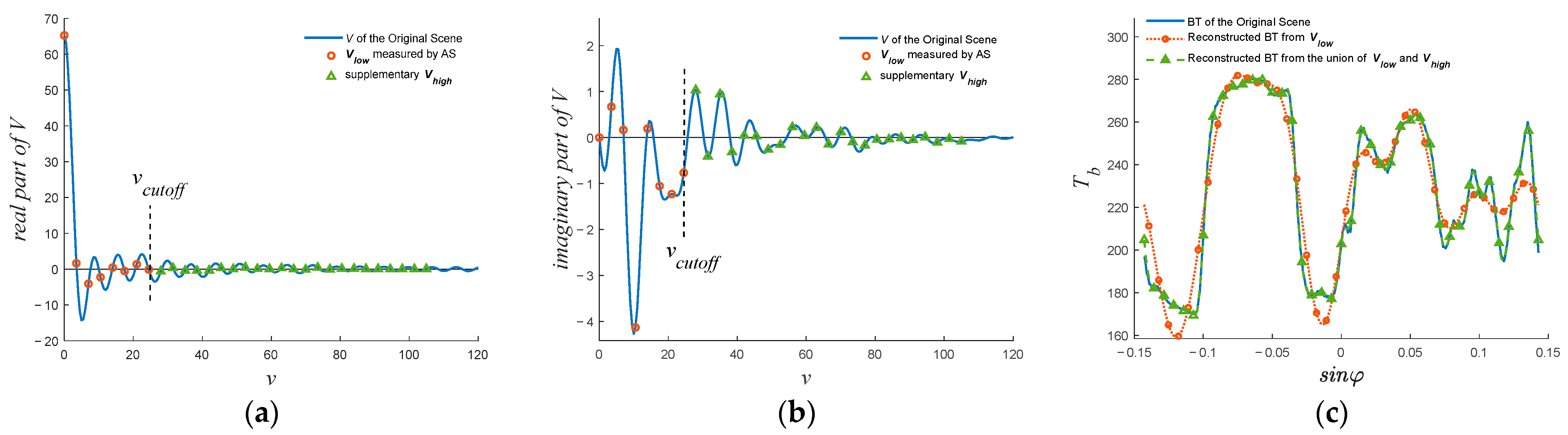
If the visibility is extended, the spatial resolution of
can be enhanced. An AS system can only obtain visibility samples at spatial frequencies lower than
(denoted as a complex vector
). If the visibility samples at spatial frequencies higher than
(denoted as a complex vector
) are added, the corresponding BT image reconstructed from the union of
and
will have higher spatial resolution and will be closer to the original BT, especially at the position where the BT changes rapidly, as illustrated in
Figure 1. Because
is added and there are more high-frequency visibility samples used in BT image reconstruction, the spatial resolution is higher. This is the theory of enhancing spatial resolution by visibility extension.
2.2. Procedure
The visibility of ordinary scenes distributes continuously; in other words, the visibility changes continuously. This implies that there is a relationship between the distribution of low- and high-frequency visibility. If the prior information of visibility distribution is learnt by a neural network, it is possible to estimate by the neural network from the obtained by an AS system.
In the VE method, a neural network is trained by the dataset generated from the visibility of various scenes to learn prior information about the visibility distribution, specifically to learn the relationship between the distribution of low- and high-frequency visibility. The trained neural network is used to estimate according to obtained by an AS system, and the estimate of is denoted as . Then, and are combined. Furthermore, the visibility samples at vn < 0 are added, and the BT image of the scene is reconstructed by the Inverse Discrete Fourier Transform (IDFT). Because high-frequency visibility samples are added in the image reconstruction, the spatial resolution of the reconstructed BT image with the VE method is higher than that of the original reconstructed BT image.
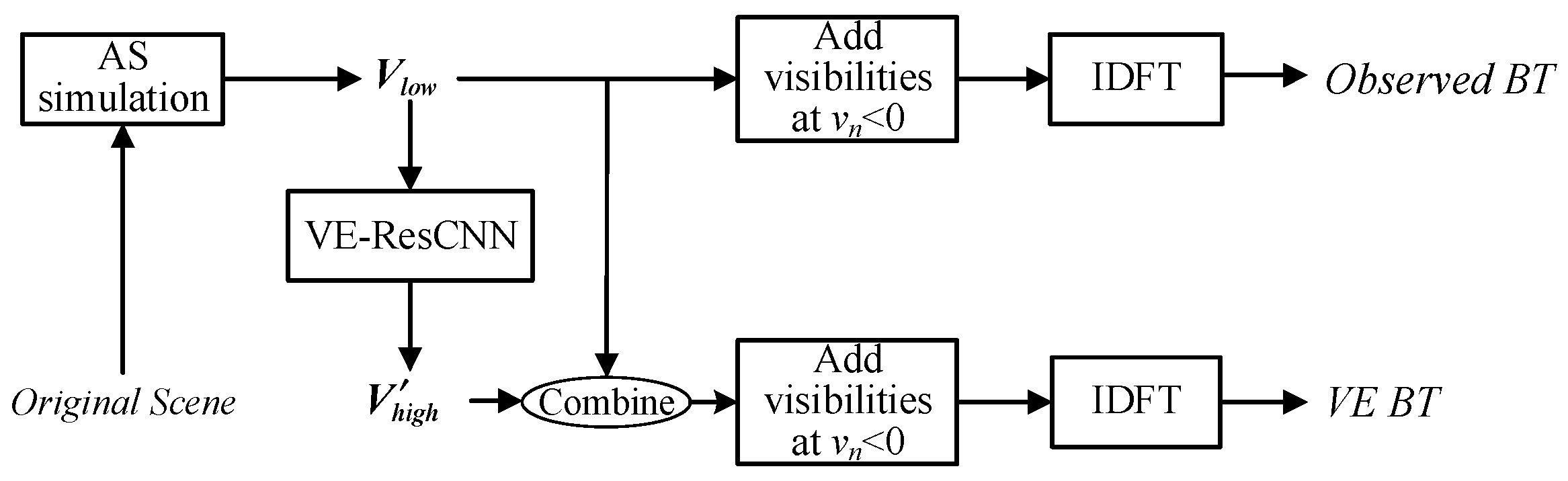
The steps of the VE method are illustrated in
Figure 2. There are five steps:
is obtained through observation by an AS system.
is output from the trained neural network with the input complex vector .
and are combined.
The visibility samples at vn < 0 are added according to .
The BT image of the scene is reconstructed by IDFT.
Figure 2.
Steps of the VE method.
Figure 2.
Steps of the VE method.
The most important step of the VE method is step 2. The dataset must be generated before the neural network is designed and trained. Then can be estimated. The dataset generation, neural network design, and network training need to be performed only once for an AS system.
2.3. Dataset
2.3.1. Procedure of Dataset Generation
The neural network needs to be trained by the dataset to determine the weights and biases. The procedure for dataset generation is listed below.
The BT image of a scene is generated. The scene can be an ideal scene or a natural scene. The BT image of an ideal scene is generated by simulation, while that of a natural scene is generated from satellite data.
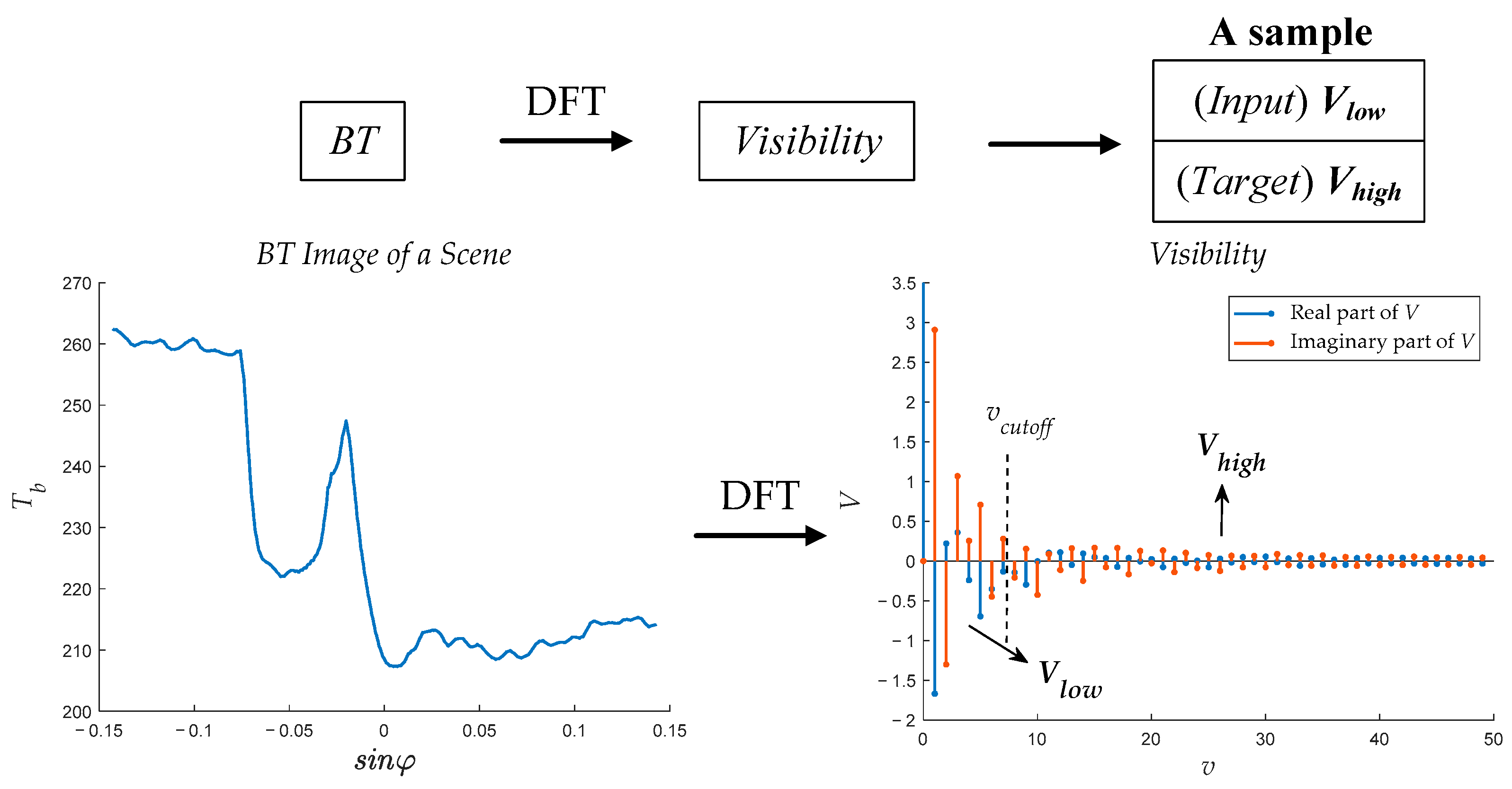
The visibility samples (where , j = 0, 1, …, n + p − 1) are acquired by a Discrete Fourier Transformation (DFT) from the scene BT according to (1).
The first
n visibility samples,
, are selected as the input complex vector
. The following
p visibility samples,
, are selected as the target complex vector
.
and
are combined into one sample, as illustrated in
Figure 3.
Multiple samples are generated by repeating steps 1 to 3, and multiple samples compose the dataset.
2.3.2. Determination of the Parameters in Dataset Generation
The parameter
n in steps 2 and 3, i.e., the length of the input complex vector
, is determined by the AS system, specifically by the number of baselines of the AS system. For the MAS-V experiment system, which has eight baselines, mentioned in
Section 4,
n = 8.
When determining the parameter
p in steps 2 and 3, i.e., the length of the output complex vector
, the balance of the spatial resolution and the reconstruction error should be considered. When
p is greater, the advantage is that there will be more high-frequency visibility samples used in the BT image reconstruction, so the spatial resolution of
is higher. However, the disadvantage is that
suffers larger reconstruction error. The reconstruction error is assessed by the root-mean-square error (
RMSE) between the reconstructed BT and the original BT of a scene, as expressed in (4).
where
is the reconstructed BT,
is the original BT, and
M is the number of the pixels of the BT image. In this article, an average reconstruction error of approximately 40,000 scenes with different values of
p was calculated, as illustrated in
Figure 4. With an increase in
p, the reconstruction error first reduced, but then increased. The value of
p should be as large as possible with an acceptable increase in
RMSE. Thus, according to
Figure 4,
p = 42 in this article, which is a trade-off.
Besides this, in step 2,
= 3.5 according to the experiment system MAS-V mentioned in
Section 4.
2.3.3. BT Images for the Dataset
According to the procedure of dataset generation described above, the first step is to generate BT images of the scenes. The BT images of numerous scenes are generated, in which two types of scene are involved: (a) ideal scenes, including scenes of point source and homogeneous scenes; (b) natural scenes, including scenes observed by the microwave radiometer carried by a satellite in orbit.
For the ideal scenes, the scenes of the point source at different locations in the field of view (FOV) are chosen, as well as homogeneous scenes with different widths and located at different positions in the FOV. BT images of ideal scenes are generated through simulation.
For the natural scenes, the scenes observed by the Scanning Microwave Radiometer (SMR) [
20] onboard HaiYang-2B (HY-2B) are chosen. The SMR was designed to measure oceanic and atmospheric parameters, such as sea-surface temperature (SST), sea-surface wind speed, water vapor, and cloud liquid water. It is a linearly polarized passive microwave radiometer that measures microwave radiation with the 6.925, 10.7, 18.7, 23.8, and 37 GHz channels, and it employs a conical scanning mechanism [
20]. In each scan, the SMR generates a 150-pixel BT image of the Earth’s surface. The SMR observation data obtained from the 37 GHz channels with horizontal and vertical polarization in February 2020 are selected and downloaded from the website (
https://osdds.nsoas.org.cn) on 12 April 2021.
For the training dataset, 9000 BT images of ideal scenes and 46,685 BT images of natural scenes are selected; and for the testing dataset, 30,589 BT images of natural scenes are selected. Some examples of the selected BT images are shown in
Figure 5.
Thus, a training dataset containing 55,658 samples and a testing dataset containing 30,589 samples are generated.
2.4. Selection of Neural Network Model
In order to find the appropriate neural network model to learn the prior information of visibility distribution and extend the visibility, the LSTM network models, the MLP network model, the CNN models, and the residual convolutional neural network (ResCNN) models are tested in this article.
In
Table 1, the parameter-search range of the architecture configuration for seven types of neural network model are presented. To generate the output with designed size, a layer (denoted as CN1), illustrated in
Figure 6, composed of two convolutional layers convolving 42 and 84 filters of 1 × 1 and a global average pooling layer, is used as the last layer of the “ResCNN + CN1” and “CNN + CN1” models; a layer (denoted as FC1) composed of two fully connected layers with 512 and 84 nodes, respectively, is used as the last layer of the “ResCNN + FC1”, “CNN + FC1”, and “LSTM + FC1” models; and a fully connected layer containing 84 nodes (denoted as FC2) is used as the last layer of the “MLP + FC2” models. Because the last layers for the models are determined, the parameter-search range presented in
Table 1 are for the layers excluding the last layer. In the table, the value of the parameter “ResCNN blocks” indicates the number of ResCNN blocks in the models; the value of the parameter “Filters” (“Nodes”) indicates the number of filters (nodes) contained in the first layer, and the number of filters (nodes) in the following layers is a multiple of the value of “Filters” (“Nodes”); the value of the parameter “Kernel size” is the size of the convolution kernel; the value of the parameter “Layers” indicates the number of layers (excluding the last layer) of the models; the value of the parameter “Units” indicates the number of features in the hidden state of LSTM.
Other hyperparameters, such as the batch size, learning rate, momentum, and dropout, are searched simultaneously. The Bayesian hyperparameter-search method is used for hyperparameter searching. The Bayesian hyperparameter-search method uses a Gaussian process to model the relationship between the parameters and the test loss, and chooses parameters to optimize the probability of improvement.
To speed up the hyperparameter search, an early termination strategy called hyperband [
21] is set to prevent poorly performing runs of the neural network models. Hyperband stopping evaluates whether a run should be stopped or permitted to continue at one or more pre-set iteration counts, which are set as the 4th, 12th, 36th, and 108th epochs in each run in this article.
For the seven types of neural network model, more than 1300 different configurations are tested in visibility extension. The training results of the most effective models in each type of neural network model are shown in
Table 2. It can be seen from
Table 2 that the ResCNN model outperforms the CNN model; the CNN model outperforms the MLP model; and the MLP model outperforms the LSTM model. The most effective of the “ResCNN + CN1” models is the most effective for visibility extension of all the tested models.
The distribution of visibility only depends on the distribution of the scene BT, so the high-frequency visibility samples have no memory of low-frequency visibility samples, which is also the reason for the poor performance of LSTM. In addition, for the general scenes, visibility distributes continuously. Therefore, there is a connection between the visibility samples at local adjacent spatial frequencies, which means that the high-frequency visibility samples are related to the low-frequency visibility samples. Compared with MLP, CNN can learn the local features of visibility distribution, which is why CNN outperforms MLP in visibility extension. For a deeper network, residual connections can reduce the impact of the degradation problem, so ResCNN performs better than other types of network model mentioned above.
Thus, the most effective of the “ResCNN + CN1” models (i.e., the VE-ResCNN) is introduced in this article and used to extend the visibility to enhance spatial resolution.
2.5. VE-ResCNN
2.5.1. Architecture
The VE-ResCNN proposed in this article is composed of 13 ResCNN blocks, a dropout layer, and a last layer (denoted as CN1), as illustrated in
Figure 6. The ResCNN blocks are used to extract the features of the input complex vector. The novelty of the residual network is in the use of the bypass pathway concept, which was employed in Highway Nets to address the problem of training a deeper network [
19]. The dropout layer is used to prevent the neural network from overfitting [
22]. In addition, the CN1 layer is used for dimensionality reduction to output the vector with the designed size.
As illustrated in
Figure 6, the network input is
, which is a complex vector with
n elements. Then, a matrix with two columns formed by the real and imaginary parts of
is input into the first ResCNN block of the VE-ResCNN.
The ResCNN block is a conventional convolutional neural network plus a residual connection. The block output, denoted as
, can be expressed as (5).
where
is the block input (when
i = 0,
is the matrix with two columns transformed from the input complex vector
), ReLU = max (0,
x) is the rectified linear unit function, and
is the output of the feed-forward network in the block, expressed as (6).
where BN is the batch-normalization process [
23],
(
) is the convolution weight matrix of the first (second) convolutional layer Conv1 (Conv2) in the ResCNN block, the symbol ∗ represents the convolution operation, and
and
are the biases.
The input of the dropout layer is the output of the ResCNN block 13. The dropout layer randomly sets some input elements to zero with a pre-set probability using samples from a Bernoulli distribution. This has been proven to be an effective technique for regularization and to prevent the co-adaptation of neurons [
24].
Then, the output matrix of the dropout layer is input into the CN1 layer. The architecture of CN1 is inspired by previous works [
25,
26]. As illustrated in
Figure 6, the kernel size of the convolutional layers (Conv1’ and Conv2’) in CN1 is 1 × 1, and the number of filters (i.e., the convolutional weight matrices) in Conv1’ and Conv2’ are
p and 2
p, respectively. Conv1’ is followed by a leaky ReLU activation whose expression is LeakyReLU (x) = max (0, x) +
f × min (0, x), where
f is the leak factor. As a substitution for a fully connected layer, the global average pooling layer can significantly reduce the number of model parameters. A vector consisting of 2
p elements is output by the CN1 layer. The output of the CN1 layer is reshaped into a two-column matrix with size 2 ×
p × 1. Then, the two columns are combined as the real and imaginary parts of a complex vector. Thus, a complex vector with the size
p × 1 (i.e.,
) is obtained.
The architecture parameters of the VE-ResCNN are listed in
Table 3. The dropout probability of the dropout layer is 0.413. In addition, the leak factor (
f) of the leaky ReLU activation in CN1 is 0.01.
2.5.2. Training
The training process of the VE-ResCNN is illustrated in
Figure 7. The mini-batch gradient descent algorithm with a momentum is used to train the VE-ResCNN.
When training the VE-ResCNN, a batch of samples is selected from the training dataset, and the input complex vectors (
) of the batch of samples are input into the VE-ResCNN. Then, the output complex vectors (
) are compared to the target complex vectors (
) of the batch of samples, and the mean-square error is calculated as the loss function according to (7).
where
S is the number of samples in the batch,
s is the serial number,
p is the length of the complex vector
(or
),
is the output complex vector corresponding to the
sth sample,
is the target complex vector corresponding to the
sth sample, real (
) is the real part of a complex vector, imag (
) is the imaginary part of a complex vector, and |
| represents the modulo of a vector.
After
Loss is calculated, the weights and biases are updated by the gradient-descent algorithm with momentum. The main disadvantage of gradient-descent learning algorithms is that they sometimes become stuck in a local minimum rather than a global minimum. Momentum is used along with the gradient-descent algorithm to solve this issue [
27].
Then, another batch of samples from the training dataset are input into the VE-ResCNN to continue the training. When all the samples in the training dataset are used, an epoch is finished. Then, the next epoch begins.
A learning-rate scheduler is employed to adjust the learning rate based on the number of epochs during training. When Loss stops decreasing for ten epochs, the learning rate is reduced by a factor of five. Learning-rate schedulers can often benefit model training.
Epoch by epoch, the weights and biases are updated iteratively to decrease Loss. When the epoch number reaches the pre-set number (NE) or Loss becomes stable, training is stopped. Thus, the training process is finished.
When training the VE-ResCNN, the batch size is set to 512; the initial learning rate is set to 0.015; the momentum is set to 0.356; and the maximum number of epochs (NE) is set to 300 in this article.
In the training process, with an increase in epoch, both the
Loss of the training dataset (denoted as train-loss) and that of the testing dataset (denoted as test-loss) first decrease, and then remain relatively stable with little effect in further training, as illustrated in
Figure 8.
The VE-ResCNN is programmed on the Pytorch framework with Python 3.9, trained on a computer with one CPU (AMD Ryzen 7 2800 H) and one GPU (NVIDIA GeForce RTX 3070). It takes approximately 4.5 h to train the VE-ResCNN for 300 epochs.
The VE-ResCNN only needs to be trained once for an AS system. The trained VE-ResCNN is then used to extend the visibility to reconstruct the BT image, which is rapid, needing less than 0.02 s, as described in a later section.
4. Experiment
The performance of the VE method is also confirmed by an experiment in this section. The experiment system MAS-V [
28,
29] is used, which was developed by Huazhong University of Science Technology (HUST). MAS-V can be used for conventional AS experiments by removal of its reflectors, as illustrated in
Figure 12. The antenna array arrangement of the system in the experiment is {1, 2, 3, 4, 5, 6, 7, 8}, and the minimum antenna spacing is 3.5
.
4.1. Experimental Procedure
The experiment procedure included four steps. Except for step 1, the other steps are the same as those of the simulation procedure described in
Section 3.1.
In step 1, the scenes in the experiment are real, which is different from the simulation. There are six scenes used to conduct the experiment: a single noise source and two noise sources 6 cm, 7 cm, 8 cm, 10 cm, and 12 cm apart. When conducting the experiment, MAS-V is used to observe the scene, and is obtained after error calibration.
4.2. Experimental Results
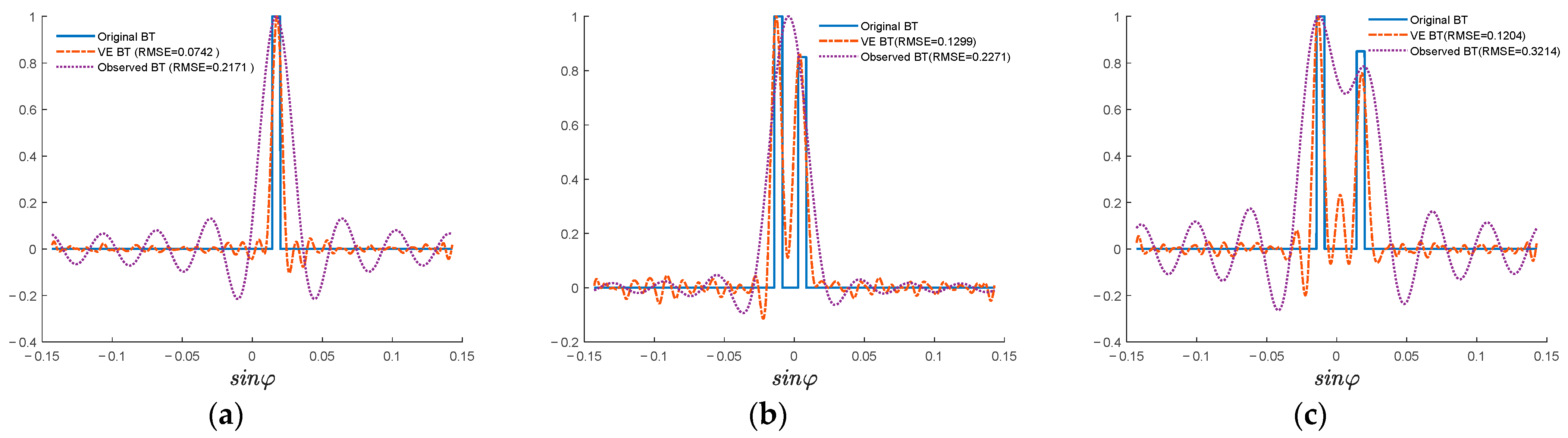
The results of the experiment are illustrated in
Figure 13. As can be seen from
Figure 13a, the HPBW of the observed BT of the single noise source is approximately 0.022 (1.26°); however, the HPBW of the VE BT of the single noise source is approximately 0.010 (0.58°), which indicates an enhancement in spatial resolution. As can be seen from
Figure 13b,e, the observed BT of dual noise sources cannot separate the two noise sources; however, the VE BT is able to, which also indicates an enhancement in spatial resolution. In addition, in
Figure 13f, although the two noise sources can be separated by both the observed BT and the VE BT, the beamwidth of the two noise sources of the VE BT is apparently narrower than that of the observed BT. These all indicate an enhancement in spatial resolution. The results are listed in
Table 7.
The time taken to reconstruct the BT image is the same as that in the simulation: 0.003 s for the observed BT image and 0.019 s for the VE BT image, shown in
Table 6.
The experiment indicates that spatial resolution can be effectively enhanced by the VE method, which is consistent with the simulation.
5. Discussion
The simulation and experiment results demonstrate that the VE method can enhance the spatial resolution of 1-D AS. Moreover, the simulation results indicate that the VE method can reduce the reconstruction error by enhancing spatial resolution.
But there are still some disadvantages and limitations of the VE method proposed in this article.
The training dataset must contain a large number of samples in order to make the prior information comprehensive for the VE-ResCNN to learn. This necessitates that there must be enough BT images of scenes to generate the dataset.
The neural network needs to be trained first to learn the prior information of visibility distribution, which means extra computational costs. The training of VE-ResCNN costs nearly 4.5 h in this article, as shown in
Table 2. Although it takes approximately 4.5 h to train the VE-ResCNN, the training process needs to be performed only once for an AS system.
However, it takes little time to perform the VE method after the neural network is trained. It takes less than 0.02 s to reconstruct a BT image, as shown in
Table 6.
6. Conclusions
The spatial resolution of AS is proportional to the size of an antenna array, which is limited by the carrying capacity of satellites. To enhance the spatial resolution of 1D-AS without increasing the size of an antenna array, the VE method is proposed in this article.
The key idea of the VE method is that the high-frequency visibility samples of a scene are estimated by VE-ResCNN from the low-frequency visibility samples observed by an AS system, and the high- and low-frequency visibility samples are combined to reconstruct the BT image of a scene to enhance the spatial resolution. Only the visibility samples at spatial frequencies lower than can be obtained by the AS system in observations. With the additional high-frequency visibility samples estimated from the low-frequency visibility samples, the spatial resolution of the reconstructed BT can be improved.
The VE-ResCNN stands out from seven types of neural network model with over 1300 different configurations. The visibility of scenes generally distributes continuously, so the visibility samples at adjacent spatial frequencies have a connection with each other. ResCNN can learn the local features more effectively than other neural networks mentioned in this article. Therefore, after training by various scenes to learn the prior information of the visibility distribution of scenes, VE-ResCNN achieves good performance in visibility extension.
The simulation indicates that the spatial resolution of 1D-AS can be effectively enhanced by the VE method; and with spatial resolution enhanced, the reconstruction error decreases by approximately 47.7%. The single noise source experiment shows that the HPBW of the single noise source of the original observed BT and the VE BT are approximately 1.26° and 0.58°, respectively. Moreover, the experiment with dual noise sources 6 cm, 7cm, 8cm, and 10 cm apart shows that the original observed BT cannot separate between the dual noise sources, although the VE BT is able to. In addition, in the experiment with dual noise sources 12 cm apart, although the two noise sources can be separated by both observed BT and VE BT, the beamwidth of VE BT is narrower than that of observed BT. These all demonstrate enhanced spatial resolution.


