
Mapping Irrigated Croplands from Sentinel-2 Images Using Deep Convolutional Neural Networks
 , , and
Abstract
:1. Introduction
2. Materials and Process
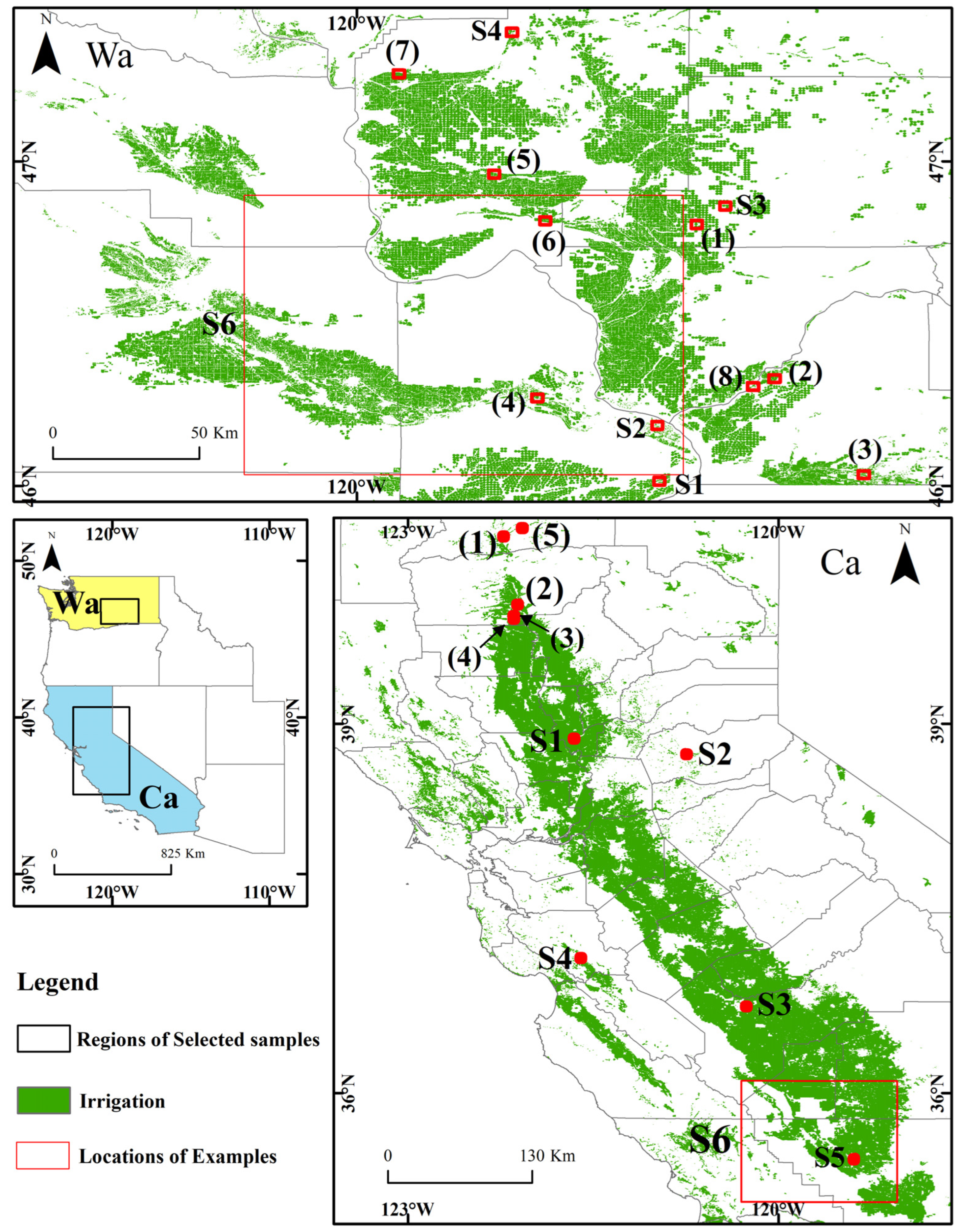
2.1. Study Areas
2.2. Collection and Pre-Processing of Remote Sensing Data
2.3. Irrigated Cropland Layer Dataset
2.4. Daymet V4 (Daily Surface Weather Data on a 1-km Grid for North America, Version 4) Precipitation Data
3. Methodology
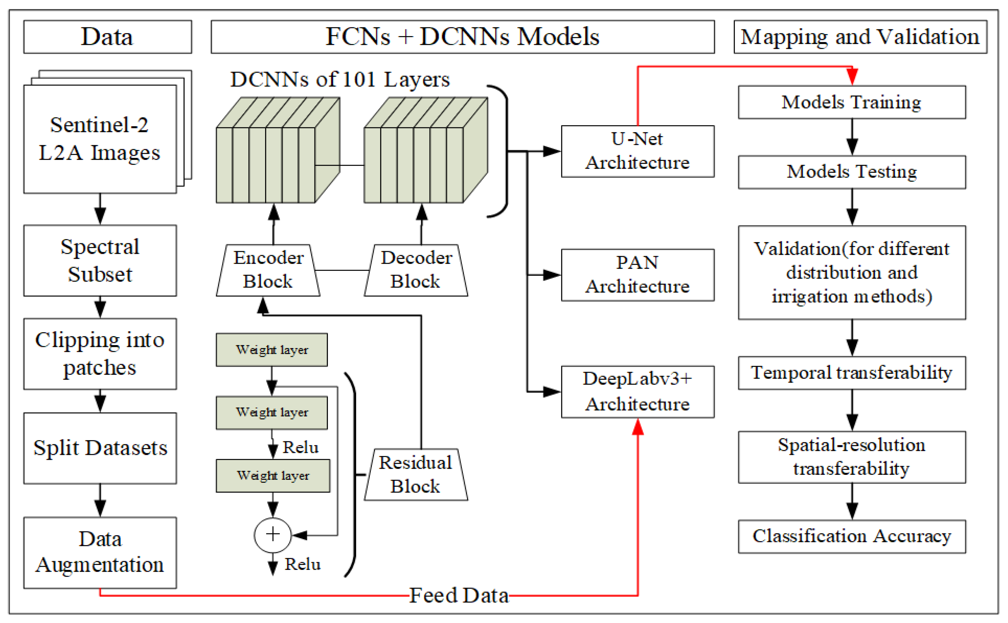
3.1. Overview
3.2. Model Design
3.3. Experiment Design
3.4. Accuracy Assessment
4. Results
4.1. Model Accuracy
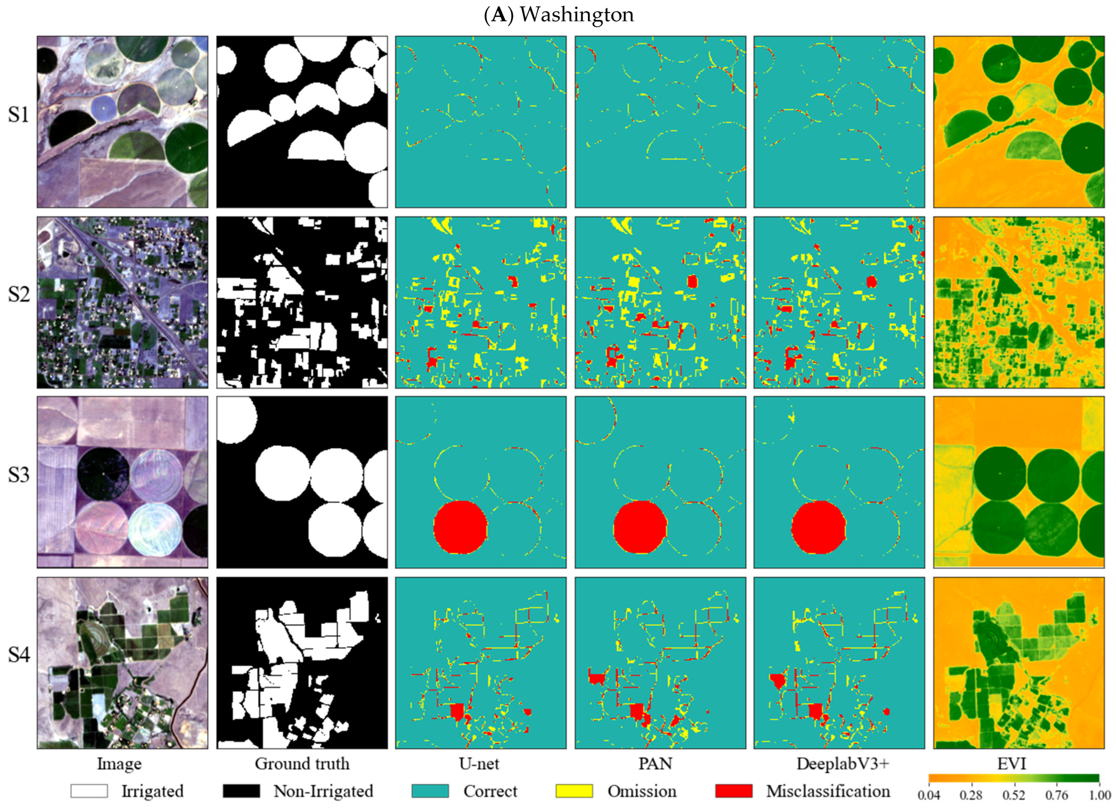
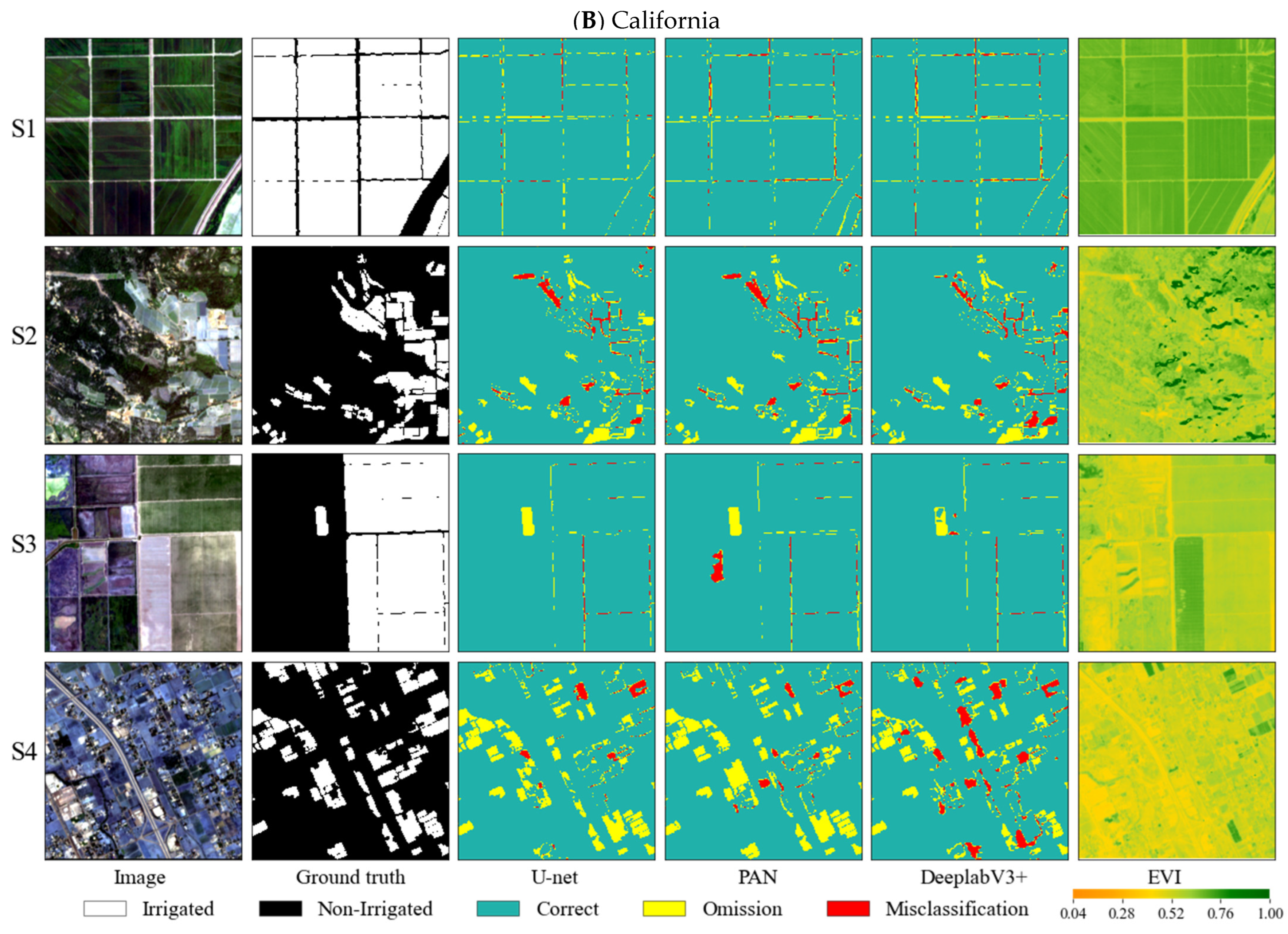
4.2. Irrigation Extraction results with Different Distribution States
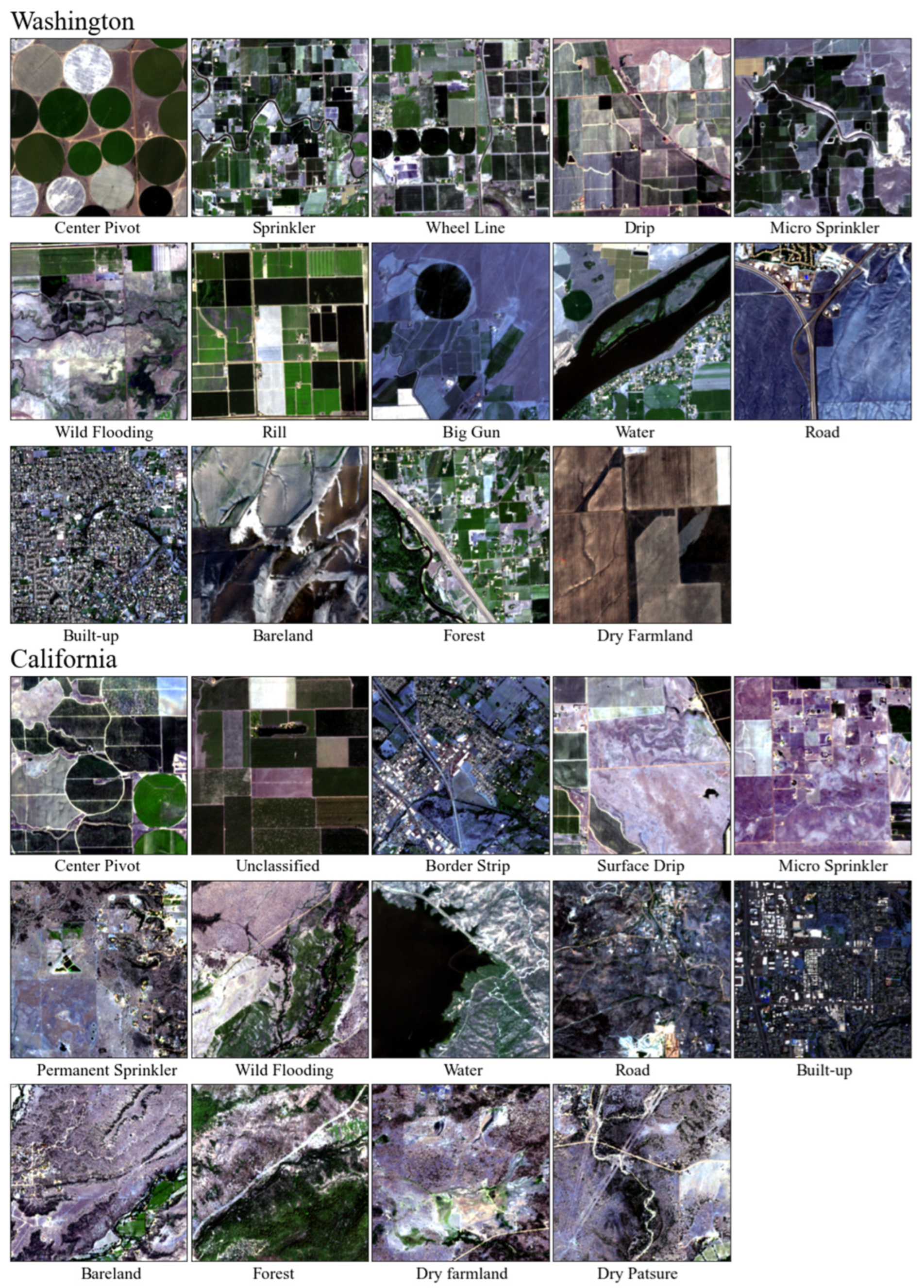
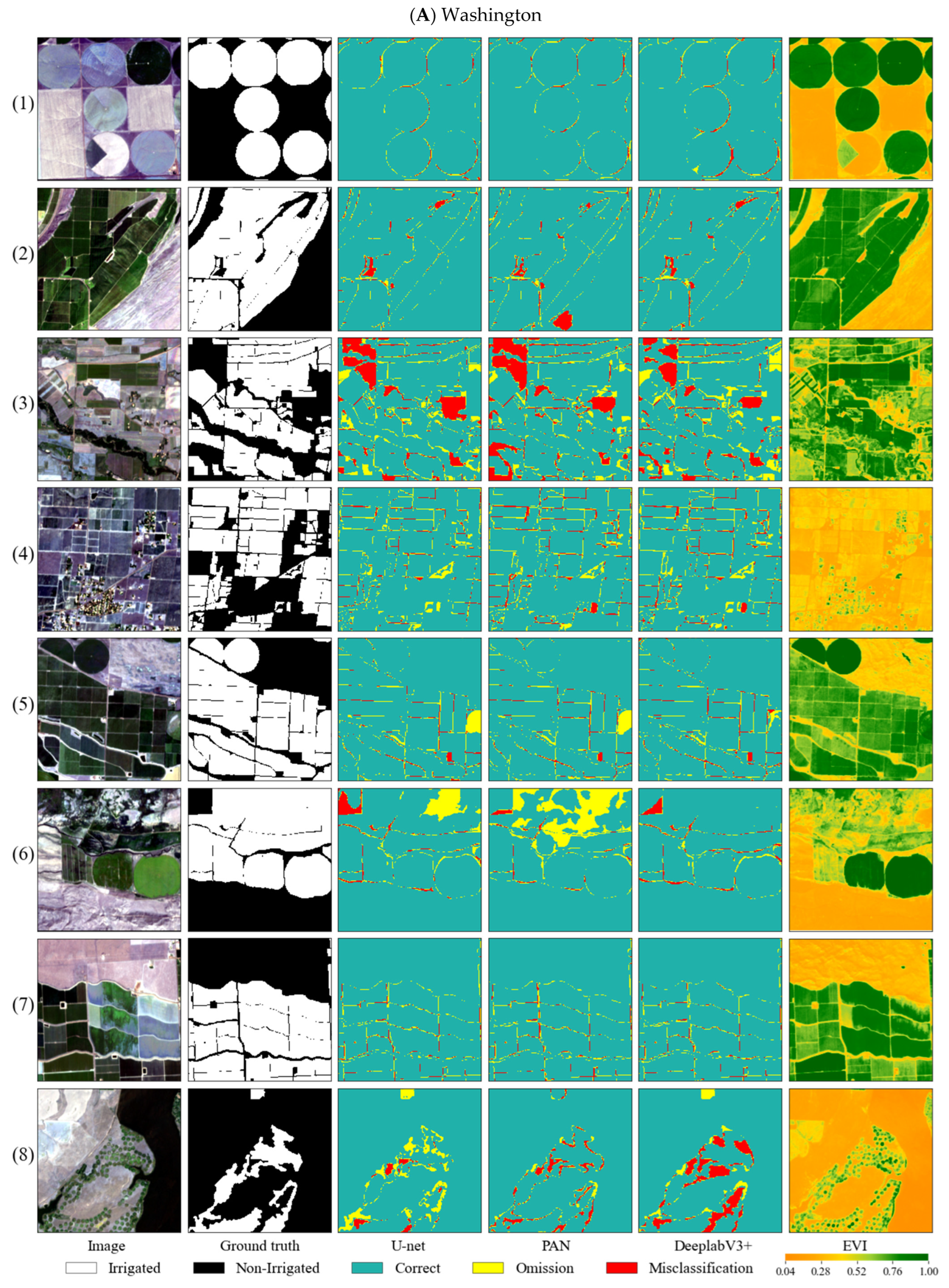
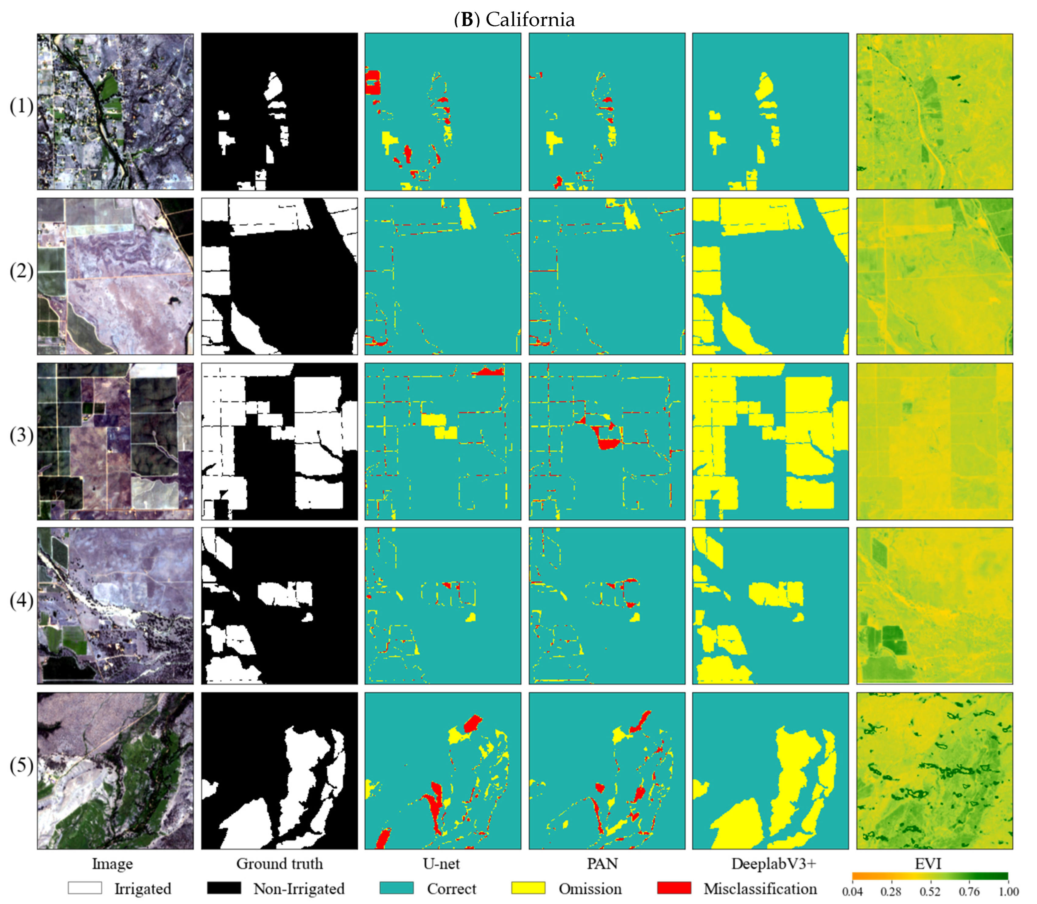
4.3. Irrigation Extraction Results among Fields Served by Different Types of Irrigation
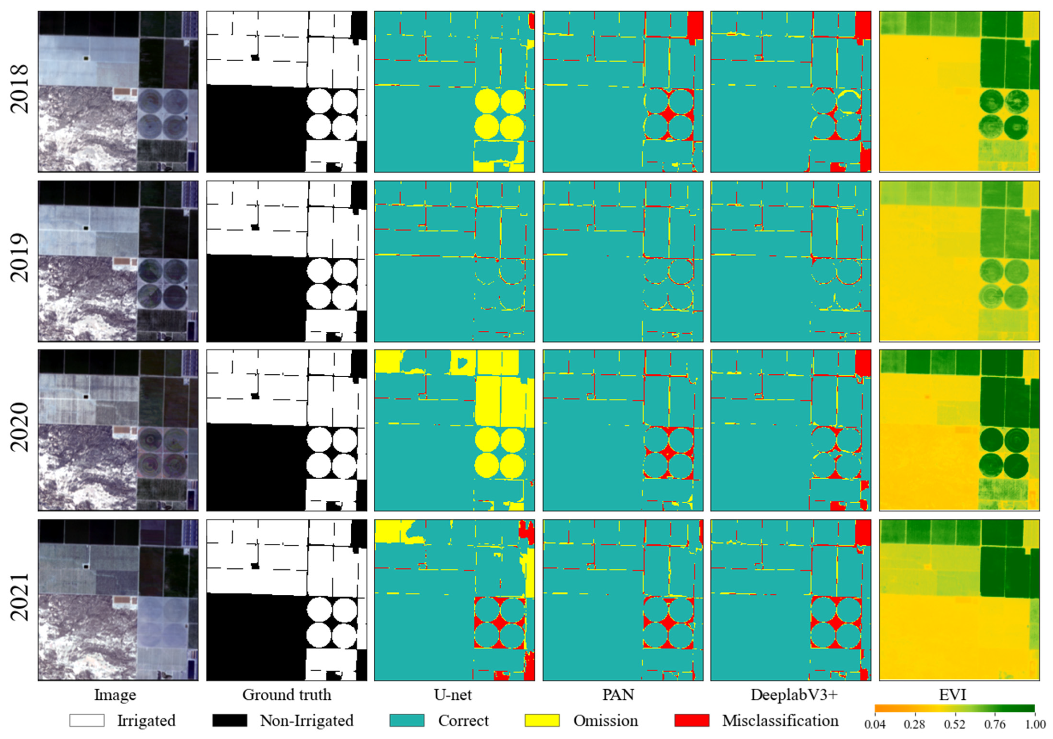
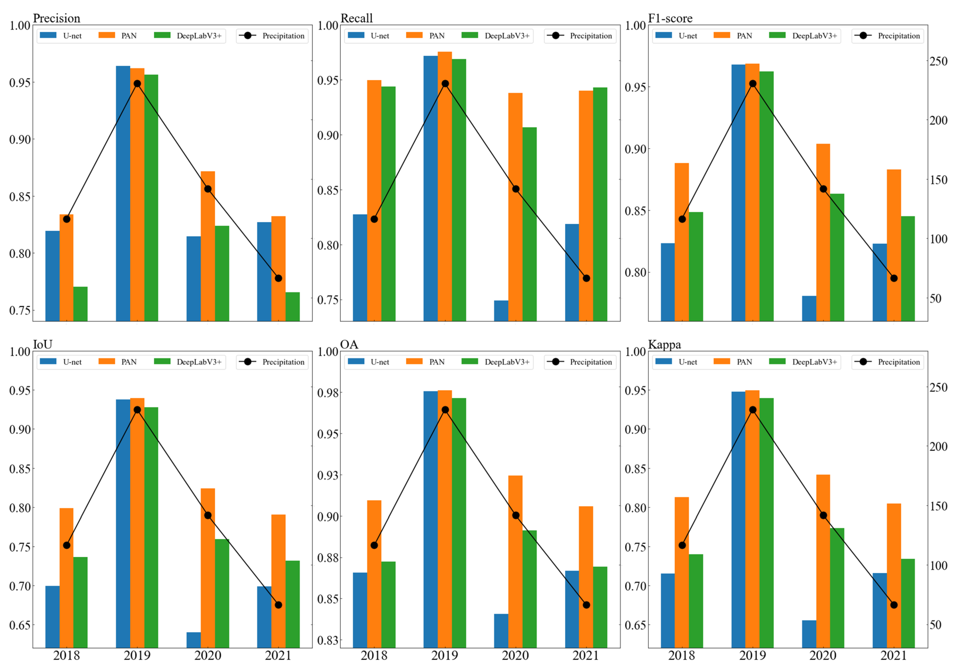
4.4. Assessment of Temporal Portability of the Deep Models to Extract Irrigation
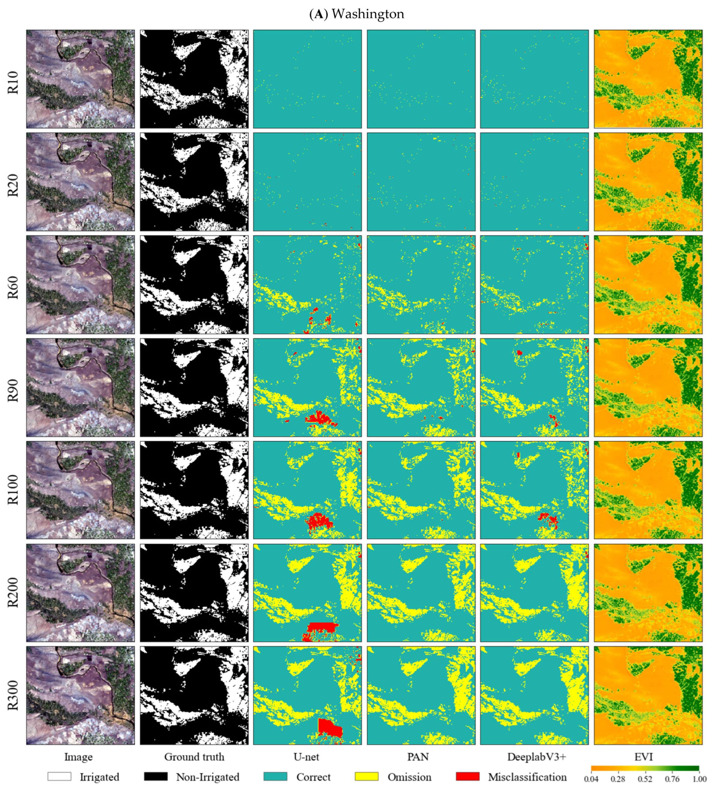
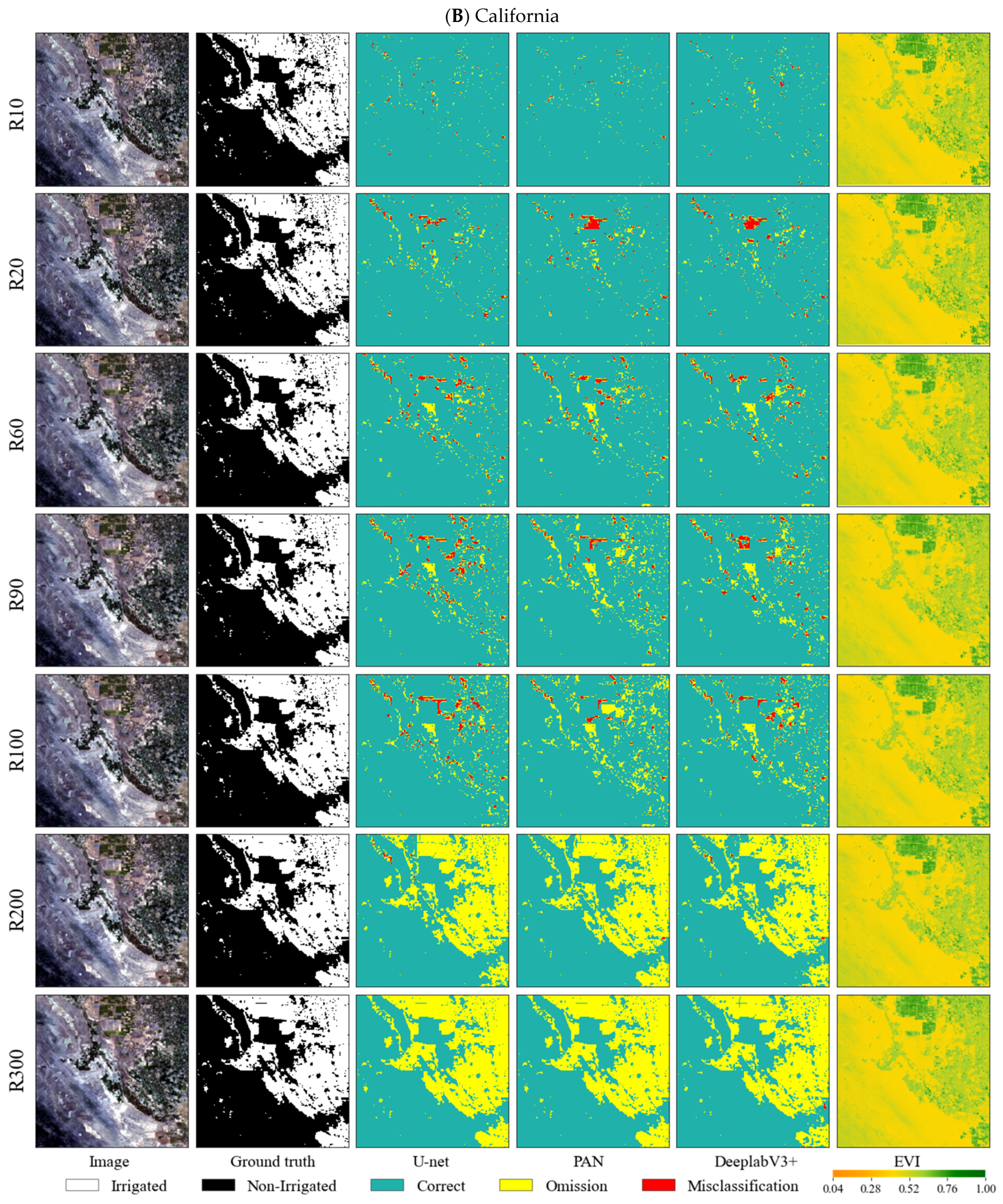
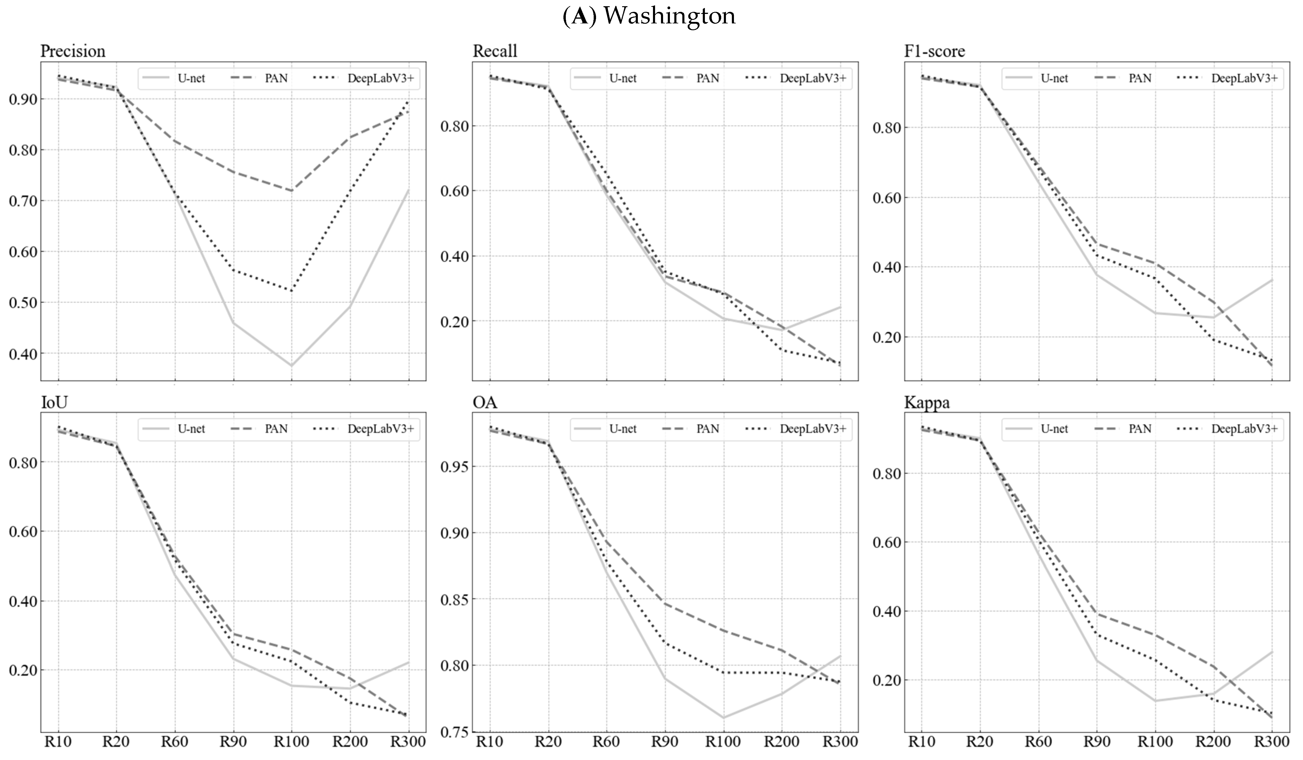
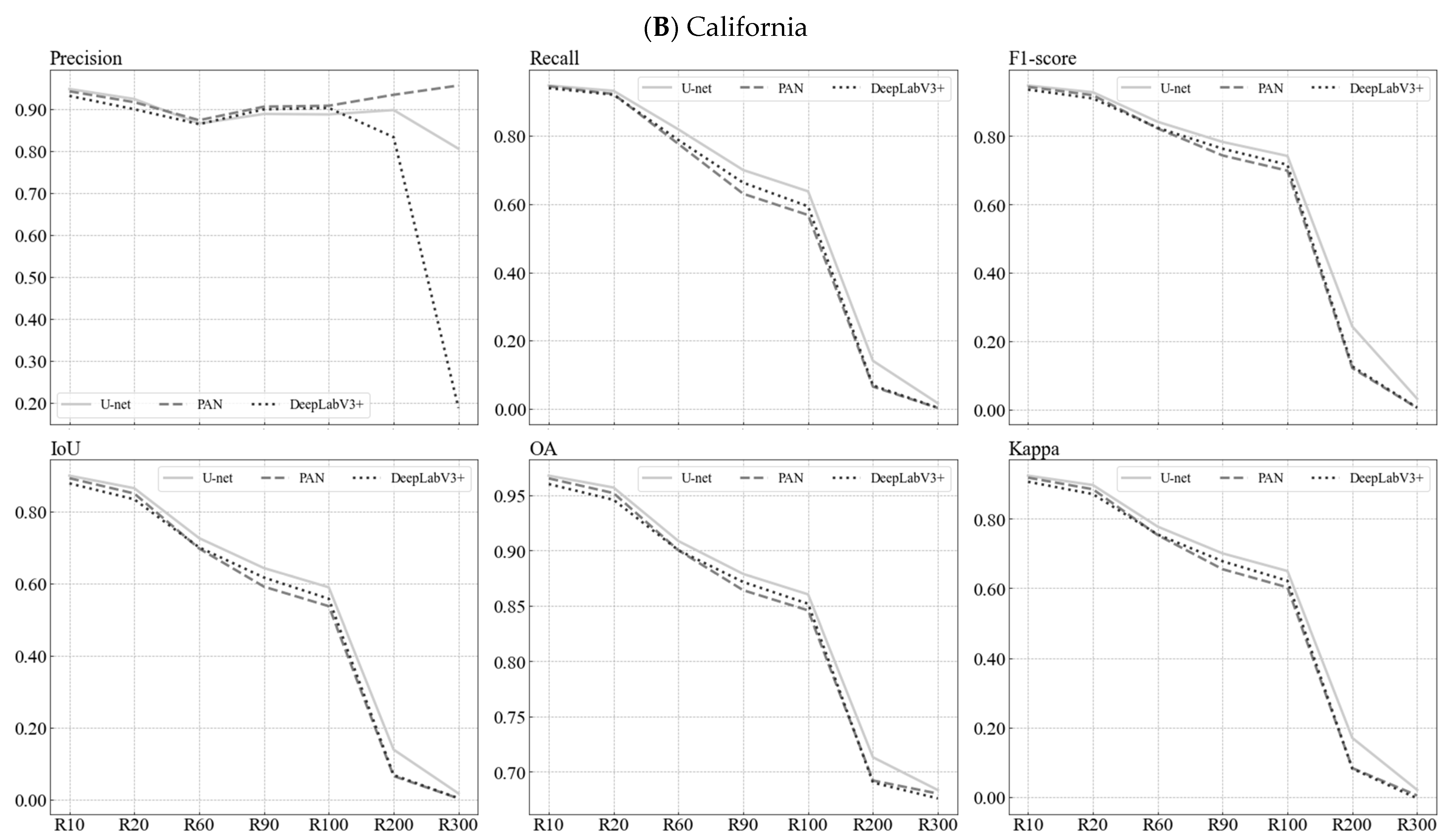
4.5. Assessment of Spatial Resolution Portability of the Deep Models to Extract Irrigation
5. Discussion
6. Conclusions
Author Contributions
Funding
Data Availability Statement
Acknowledgments
Conflicts of Interest
References
- Wada, Y.; Wisser, D.; Eisner, S.; Flörke, M.; Gerten, D.; Haddeland, I.; Hanasaki, N.; Masaki, Y.; Portmann, F.T.; Stacke, T.; et al. Multimodel projections and uncertainties of irrigation water demand under climate change. Geophys. Res. Lett. 2013, 40, 4626–4632. [Google Scholar] [CrossRef]
- Cherlet, M.; Hutchinson, C.; Reynolds, J.; Hill, J.; Sommer, S.; von Maltitz, G. World Atlas of Desertification; Publication Office of the European Union: Luxembourg, 2018; p. 56.
- Zhong, C.; Guo, H.; Swan, I.; Gao, P.; Yao, Q.; Li, H. Evaluating trends, profits, and risks of global cities in recent urban expansion for advancing sustainable development. Habitat Int. 2023, 138, 102869. [Google Scholar] [CrossRef]
- Loveland, T.R.; Reed, B.C.; Brown, J.F.; Ohlen, D.O.; Zhu, Z.; Yang, L.; Merchant, J.W. Development of a global land cover characteristics database and IGBP DISCover from 1 km AVHRR data. Int. J. Remote Sens. 2000, 21, 1303–1330. [Google Scholar] [CrossRef]
- Bartholomé, E.; Belward, A.S. GLC2000: A new approach to global land cover mapping from Earth observation data. Int. J. Remote Sens. 2005, 26, 1959–1977. [Google Scholar] [CrossRef]
- Defourny, P.; Bicheron, P.; Brockman, C.; Bontemps, S.; Van, B.E.; Pekel, J.; Arino, O. The first 300 m global land cover map for 2005 using ENVISAT MERIS time series: A product of the GlobCover system. In Proceedings of the 33rd International Symposium on Remote Sensing of Environment, Stresa, Italy, 4–8 May 2009. [Google Scholar]
- Alijafar, M.; Jamal, J.A. Insights on the historical and emerging global land cover changes: The case of ESA-CCI-LC datasets. Appl. Geogr. 2019, 106, 82–92. [Google Scholar]
- Zhang, X.; Liu, L.; Chen, X.; Gao, Y.; Xie, S.; Mi, J. GLC_FCS30: Global land-cover product with fine classification system at 30 m using time-series Landsat imagery. Earth Syst. Sci. Data 2021, 13, 2753–2776. [Google Scholar] [CrossRef]
- Siebert, S.; Kummu, M.; Porkka, M.; Döll, P.; Ramankutty, N.; Scanlon, B.R. A global data set of the extent of irrigated land from 1900 to 2005. Hydrol. Earth Syst. Sci. 2015, 19, 1521–1545. [Google Scholar] [CrossRef]
- Prasad, S.; Chandrashekhar, M.B.; Praveen, N.; Venkateswarlu, D.; Yuanjie, L.; Muralikrishna, G. Global irrigated area map (GIAM), derived from remote sensing, for the end of the last millennium. Int. J. Remote Sens. 2009, 30, 3679–3733. [Google Scholar]
- Salmon, J.M.; Mark, A.F.; Steve, F.; Dominik, W.; Ellen, M.D. Global rain-fed, irrigated, and paddy croplands: A new high-resolution map derived from remote sensing, crop inventories and climate data. Int. J. Appl. Earth Obs. Geoinf. 2015, 38, 321–334. [Google Scholar] [CrossRef]
- Teluguntla, P.; Thenkabail, P.S.; Xiong, J.; Gumma, M.K.; Giri, C.; Milesi, C.; Ozdogan, M.; Congalton, R.; Tilton, J.; Sankey, T.T.; et al. Global Cropland Area Database (GCAD) derived from remote sensing in support of food security in the twenty-first century: Current achievements and future possibilities. In Land Resources Monitoring, Modeling, and Mapping with Remote Sensing (Remote Sensing Handbook); Taylor & Francis: Boca Raton, FL, USA, 2015; pp. 1–45. [Google Scholar]
- Gumma, M.K.; Thenkabail, P.S.; Teluguntla, P.G.; Oliphant, A.; Xiong, J.; Giri, C.; Pyla, V.; Dixit, S.; Whitbread, A.M. Agricultural cropland extent and areas of South Asia derived using Landsat satellite 30-m time-series big-data using random forest machine learning algorithms on the Google Earth Engine cloud. GISci. Remote Sens. 2020, 57, 302–322. [Google Scholar] [CrossRef]
- Brown, J.F.; Pervez, M.S. Merging remote sensing data and national agricultural statistics to model change in irrigated agriculture. Agric. Syst. 2014, 127, 28–40. [Google Scholar] [CrossRef]
- Zhang, C.; Dong, J.; Zuo, L.; Ge, Q. Tracking spatiotemporal dynamics of irrigated croplands in China from 2000 to 2019 through the synergy of remote sensing, statistics, and historical irrigation datasets. Agric. Water Manag. 2022, 263, 107458. [Google Scholar] [CrossRef]
- Deines, J.M.; Kendall, A.D.; Hyndman, D.W. Annual irrigation dynamics in the U.S. northern High Plains derived from Landsat satellite data. Geophys. Res. Lett. 2017, 44, 9350–9360. [Google Scholar] [CrossRef]
- Xie, Y.; Lark, T.J.; Brown, J.F.; Gibbs, H.K. Mapping irrigated cropland extent across the conterminous United States at 30 m resolution using a semi-automatic training approach on Google earth engine. ISPRS J. Photogramm. Remote Sens. 2019, 155, 136–149. [Google Scholar] [CrossRef]
- Xie, Y.; Lark, T.J. Mapping annual irrigation from Landsat imagery and environmental variables across the conterminous United States. Remote Sens. Environ. 2021, 260, 112445. [Google Scholar] [CrossRef]
- Ren, J.; Shao, Y.; Wan, H.; Xie, Y.; Campos, A. A two-step mapping of irrigated corn with multi-temporal MODIS and Landsat analysis ready data. ISPRS J. Photogramm. Remote Sens. 2021, 176, 69–82. [Google Scholar] [CrossRef]
- Magidi, J.; Nhamo, L.; Mpandeli, S.; Mabhaudhi, T. Application of the random forest classifier to map irrigated areas using google earth engine. Remote Sens. 2021, 13, 876. [Google Scholar] [CrossRef]
- Yao, Z.; Cui, Y.; Geng, X.; Chen, X.; Li, S. Mapping Irrigated Area at Field Scale Based on the OPtical TRApezoid Model (OPTRAM) Using Landsat Images and Google Earth Engine. IEEE Trans. Geosci. Remote Sens. 2022, 60, 4409011. [Google Scholar] [CrossRef]
- Bazzi, H.; Baghdadi, N.; Amin, G.; Fayad, I.; Zribi, M.; Demarez, V.; Belhouchette, H. An Operational Framework for Mapping Irrigated Areas at Plot Scale Using Sentinel-1 and Sentinel-2 Data. Remote Sens. 2021, 13, 2584. [Google Scholar] [CrossRef]
- Demarez, V.; Helen, F.; Marais-Sicre, C.; Baup, F. In-season mapping of irrigated crops using Landsat 8 and Sentinel-1 time series. Remote Sens. 2019, 11, 118. [Google Scholar] [CrossRef]
- Zurqani, H.A.; Allen, J.S.; Post, C.J.; Pellett, C.A.; Walker, T.C. Mapping and quantifying agricultural irrigation in heterogeneous landscapes using Google Earth Engine. Remote Sens. Appl. Soc. Environ. 2021, 23, 100590. [Google Scholar] [CrossRef]
- Vogels, M.F.; de Jong, S.M.; Sterk, G.; Addink, E.A. Mapping irrigated agriculture in complex landscapes using SPOT6 imagery and object-based image analysis—A case study in the Central Rift Valley, Ethiopia-. Int. J. Appl. Earth Obs. Geoinf. 2019, 75, 118–129. [Google Scholar] [CrossRef]
- Bazzi, H.; Baghdadi, N.; El Hajj, M.; Zribi, M.; Minh, D.H.; Ndikumana, E.; Courault, D.; Belhouchette, H. Mapping paddy rice using Sentinel-1 SAR time series in Camargue, France. Remote Sens. 2019, 7, 887. [Google Scholar] [CrossRef]
- Bazzi, H.; Baghdadi, N.; Ienco, D.; El Hajj, M.; Zribi, M.; Belhouchette, H.; Escorihuela, M.J.; Demarez, V. Mapping irrigated areas using Sentinel-1 time series in Catalonia, Spain. Remote Sens. 2019, 15, 1836. [Google Scholar] [CrossRef]
- Bazzi, H.; Baghdadi, N.; Fayad, I.; Zribi, M.; Belhouchette, H.; Demarez, V. Near real-time irrigation detection at plot scale using sentinel-1 data. Remote Sens. 2020, 9, 1456. [Google Scholar] [CrossRef]
- Bazzi, H.; Baghdadi, N.; Fayad, I.; Charron, F.; Zribi, M.; Belhouchette, H. Irrigation events detection over Intensively irrigated grassland plots using Sentinel-1 data. Remote Sens. 2020, 24, 4058. [Google Scholar] [CrossRef]
- Bazzi, H.; Ienco, D.; Baghdadi, N.; Zribi, M.; Demarez, V. Distilling before refine: Spatio-temporal transfer learning for mapping irrigated areas using Sentinel-1 time series. IEEE Geosci. Remote Sens. Lett. 2020, 11, 1909–1913. [Google Scholar] [CrossRef]
- Bazzi, H.; Baghdadi, N.; Charron, F.; Zribi, M. Comparative Analysis of the Sensitivity of SAR Data in C and L Bands for the Detection of Irrigation Events. Remote Sens. 2022, 10, 2312. [Google Scholar] [CrossRef]
- Bazzi, H.; Baghdadi, N.; Zribi, M. Comparative Analysis between Two Operational Irrigation Mapping Models over Study Sites in Mediterranean and Semi-Oceanic Regions. Water 2022, 9, 1341. [Google Scholar] [CrossRef]
- Bazzi, H.; Baghdadi, N.; Najem, S.; Jaafar, H.; Le Page, M.; Zribi, M.; Faraslis, I.; Spiliotopoulos, M. Detecting irrigation events over semi-arid and temperate climatic areas using Sentinel-1 data: Case of several summer crops. Agronomy 2022, 11, 2725. [Google Scholar] [CrossRef]
- Sisodia, P.S.; Tiwari, V.; Kumar, A. Analysis of supervised maximum likelihood classification for remote sensing image. In Proceedings of the International Conference on Recent Advances and Innovations in Engineering (ICRAIE-2014), Jaipur, India, 9–11 May 2014; Volume 5, p. 11. [Google Scholar]
- Gislason, P.O.; Benediktsson, J.A.; Sveinsson, J.R. Random forest classification of multisource remote sensing and geographic data. In Proceedings of the IGARSS 2004, 2004 IEEE International Geoscience and Remote Sensing Symposium, Anchorage, AK, USA, 20–24 September 2004; Volume 9, p. 24. [Google Scholar]
- Mountrakis, G.; Im, J.; Ogole, C. Support vector machines in remote sensing: A review. ISPRS J. Photogramm. Remote Sens. 2011, 66, 247–259. [Google Scholar] [CrossRef]
- Gardner, M.W.; Dorling, S.R. Artificial neural networks (the multilayer perceptron)—A review of applications in the atmospheric sciences. Atmos. Environ. 1998, 32, 2627–2636. [Google Scholar] [CrossRef]
- Zhong, Y.; Wu, S.; Zhao, B. Scene semantic understanding based on the spatial context relations of multiple objects. Remote Sens. 2017, 9, 1030. [Google Scholar] [CrossRef]
- Hu, F.; Xia, G.S.; Zhang, L. Deep sparse representations for land-use scene classification in remote sensing images. In Proceedings of the 2016 IEEE 13th International Conference on Signal Processing (ICSP), Chengdu, China, 6–10 November 2016; Volume 11, p. 10. [Google Scholar]
- Tong, X.Y. Large-Scale Land-Cover Classification with High-Resolution Remote Sensing Images. Ph.D. Thesis, Wuhan University, Wuhan, China, 2020. [Google Scholar]
- Hu, J.; Xia, G.S.; Hu, F. A comparative study of sampling analysis in the scene classification of optical high-spatial resolution remote sensing imagery. Remote Sens. 2015, 7, 14988–15013. [Google Scholar] [CrossRef]
- Boulila, W.; Sellami, M.; Driss, M.; Al-Sarem, M.; Safaei, M.; Ghaleb, F.A. RS-DCNN: A novel distributed convolutional-neural-networks based-approach for big remote-sensing image classification. Comput. Electron. Agric. 2021, 182, 106014. [Google Scholar] [CrossRef]
- Yuan, Q.; Shen, H.; Li, T.; Li, Z.; Li, S.; Jiang, Y.; Xu, H.; Tan, W.; Yang, Q.; Wang, J.; et al. Deep learning in environmental remote sensing: Achievements and challenges. Remote Sens. Environ. 2020, 241, 111716. [Google Scholar] [CrossRef]
- LeCun, Y.; Bottou, L.; Bengio, Y.; Haffner, P. Gradient-based learning applied to document recognition. Proc. IEEE. 1998, 86, 2278–2324. [Google Scholar] [CrossRef]
- Krizhevsky, A.; Sutskever, I.; Hinton, G.E. Imagenet classification with deep convolutional neural networks. Commun. ACM 2017, 60, 84–90. [Google Scholar] [CrossRef]
- Chatfield, K.; Simonyan, K.; Vedaldi, A.; Zisserman, A. Return of the devil in the details: Delving deep into convolutional nets. arXiv 2014, arXiv:1405.3531. [Google Scholar]
- Simonyan, K.; Zisserman, A. Very deep convolutional networks for large-scale image recognition. arXiv 2014, arXiv:1409.1556. [Google Scholar]
- Szegedy, C.; Liu, W.; Jia, Y.; Sermanet, P.; Reed, S.; Anguelov, D.; Erhan, D.; Vanhoucke, V.; Rabinovich, A. Going deeper with convolutions. In Proceedings of the IEEE Conference on Computer Vision and Pattern Recognition (CVPR), Boston, MA, USA, 7–12 June 2015; pp. 1–9. [Google Scholar]
- Zhang, C.; Sargent, I.; Pan, X.; Li, H.; Gardiner, A.; Hare, J.; Atkinson, P.M. An object-based convolutional neural network (OCNN) for urban land use classification. Remote Sens. Environ. 2018, 216, 57–70. [Google Scholar] [CrossRef]
- Ronneberger, O.; Fischer, P.; Brox, T. U-Net: Convolutional Networks for Biomedical Image Segmentation. In Proceedings of the Medical Image Computing and Computer-Assisted Intervention–MICCAI 2015: 18th International Conference, Munich, Germany, 5–9 October 2015. [Google Scholar]
- Yang, M.; Yuan, Y.; Liu, G. SDUNet: Road Extraction via Spatial Enhanced and Densely Connected UNet. Pattern Recognit. 2022, 126, 108549. [Google Scholar] [CrossRef]
- Graf, L.; Bach, H.; Tiede, D. Semantic segmentation of Sentinel-2 imagery for mapping irrigation center pivots. Remote Sens. 2020, 12, 3937. [Google Scholar] [CrossRef]
- Saraiva, M.; Protas, É.; Salgado, M.; Souza, C., Jr. Automatic mapping of center pivot irrigation systems from satellite images using deep learning. Remote Sens. 2020, 12, 558. [Google Scholar] [CrossRef]
- Sun, C.; Shrivastava, A.; Singh, S.; Gupta, A. Revisiting unreasonable effectiveness of data in deep learning era. In Proceedings of the IEEE International Conference on Computer Vision (ICCV), Venice, Italy, 22–29 October 2017; pp. 843–852. [Google Scholar]
- Zhu, X.X.; Tuia, D.; Mou, L.; Xia, G.; Zhang, L.; Xu, F.; Fraundorfer, F. Deep learning in remote sensing: A comprehensive review and list of resources. IEEE Geosci. Remote Sens. 2017, 5, 8–36. [Google Scholar] [CrossRef]
- Washington State Department of Agriculture, Washington Agriculture Land Use. Available online: https://agr.wa.gov/departments/land-and-water/natural-resources/agricultural-land-use (accessed on 5 April 2023).
- Statewide Crop Mapping. California Department of Water Resources. Available online: https://data.cnra.ca.gov/dataset/statewide-crop-mapping (accessed on 3 April 2023).
- USDA-NASS. 2018 Irrigation and Water Management Survey; USDA: Washington, DC, USA, 2019; Volume 3, p. 7.
- Colligan, T.; Ketchum, D.; Brinkerhoff, D.; Maneta, M. A Deep Learning Approach to Mapping Irrigation Using Landsat: IrrMapper U-Net. IEEE Trans. Geosci. Remote Sens. 2022, 60, 4411611. [Google Scholar] [CrossRef]
- Ketchum, D.; Jencso, K.; Maneta, M.P.; Melton, F.; Jones, M.O.; Huntington, J. IrrMapper: A machine learning approach for high resolution mapping of irrigated agriculture across the Western US. Remote Sens. 2020, 12, 2328. [Google Scholar] [CrossRef]
- Thornton, M.M.R.; Shrestha, Y.; Wei, P.E.; Thornton, S.K.; Wilson, B.E. Daymet: Daily Surface Weather Data on a 1-km Grid for North America, Version 4; ORNL DAAC: Oak Ridge, TN, USA, 2020. [CrossRef]
- Li, H.; Xiong, P.; An, J.; Wang, L. Pyramid Attention Network for Semantic Segmentation. arXiv 2018, arXiv:1805.10180. [Google Scholar]
- Chen, L.C.; Zhu, Y.; Papandreou, G.; Schroff, F.; Adam, H. Encoder-decoder with atrous separable convolution for semantic image segmentation. In Proceedings of the European Conference on Computer Vision (ECCV), Munich, Germany, 8–14 September 2018; pp. 801–818. [Google Scholar]
- Zhang, C.; Dong, J.W.; Ge, Q.S. Mapping 20 years of irrigated croplands in China using MODIS and statistics and existing irrigation products. Sci. Data 2022, 9, 407. [Google Scholar] [CrossRef] [PubMed]
- Yan, H.M.; Fu, Y.L.; Xiao, X.M.; Huang, H.Q.; He, H.L.; Ediger, L. Modeling gross primary productivity for winter wheat–maize double cropping system using MODIS time series and CO2 eddy flux tower data. Agric. Ecosyst. Environ. 2009, 129, 391–400. [Google Scholar] [CrossRef]


| Washington | California | |||||||||||
|---|---|---|---|---|---|---|---|---|---|---|---|---|
| Precision | Recall | F1-Score | IoU | OA | Kappa | Precision | Recall | F1-Score | IoU | OA | Kappa | |
| DeepLabV3+ | 0.94 | 0.95 | 0.95 | 0.90 | 0.98 | 0.94 | 0.93 | 0.94 | 0.94 | 0.88 | 0.96 | 0.91 |
| PAN | 0.94 | 0.94 | 0.94 | 0.89 | 0.98 | 0.93 | 0.94 | 0.95 | 0.94 | 0.89 | 0.97 | 0.92 |
| U-net | 0.94 | 0.95 | 0.94 | 0.89 | 0.98 | 0.93 | 0.95 | 0.95 | 0.95 | 0.90 | 0.97 | 0.92 |
| Washington | California | |||||||||||
|---|---|---|---|---|---|---|---|---|---|---|---|---|
| Precision | Recall | F1-Score | IoU | OA | Kappa | Precision | Recall | F1-Score | IoU | OA | Kappa | |
| DeepLabV3+ | 0.98 | 0.98 | 0.98 | 0.96 | 0.97 | 0.94 | 0.98 | 0.93 | 0.96 | 0.92 | 0.93 | 0.91 |
| PAN | 0.98 | 0.98 | 0.98 | 0.96 | 0.98 | 0.94 | 0.98 | 0.92 | 0.95 | 0.91 | 0.92 | 0.92 |
| U-net | 0.98 | 0.98 | 0.98 | 0.95 | 0.97 | 0.93 | 0.98 | 0.93 | 0.96 | 0.92 | 0.93 | 0.92 |
| Washington | California | |||||||
|---|---|---|---|---|---|---|---|---|
| Examples | S1 | S2 | S3 | S4 | S1 | S2 | S3 | S4 |
| Precipitation | 164.6 | 100.25 | 135.9 | 109.56 | 584.26 | 973.57 | 155.49 | 421.74 |
| Washington | California | ||||||||||||
|---|---|---|---|---|---|---|---|---|---|---|---|---|---|
| Examples | (1) | (2) | (3) | (4) | (5) | (6) | (7) | (8) | (1) | (2) | (3) | (4) | (5) |
| Precipitation | 127.11 | 187.48 | 265.90 | 95.60 | 91.85 | 80.63 | 92.65 | 149.20 | 699.08 | 597.81 | 597.69 | 600.20 | 830.91 |
Disclaimer/Publisher’s Note: The statements, opinions and data contained in all publications are solely those of the individual author(s) and contributor(s) and not of MDPI and/or the editor(s). MDPI and/or the editor(s) disclaim responsibility for any injury to people or property resulting from any ideas, methods, instructions or products referred to in the content. |
© 2023 by the authors. Licensee MDPI, Basel, Switzerland. This article is an open access article distributed under the terms and conditions of the Creative Commons Attribution (CC BY) license (https://creativecommons.org/licenses/by/4.0/).
Share and Cite
Li, W.; Sun, Y.; Zhou, Y.; Gong, L.; Li, Y.; Xin, Q. Mapping Irrigated Croplands from Sentinel-2 Images Using Deep Convolutional Neural Networks. Remote Sens. 2023, 15, 4071. https://doi.org/10.3390/rs15164071
Li W, Sun Y, Zhou Y, Gong L, Li Y, Xin Q. Mapping Irrigated Croplands from Sentinel-2 Images Using Deep Convolutional Neural Networks. Remote Sensing. 2023; 15(16):4071. https://doi.org/10.3390/rs15164071
Chicago/Turabian StyleLi, Wei, Ying Sun, Yanqing Zhou, Lu Gong, Yaoming Li, and Qinchuan Xin. 2023. "Mapping Irrigated Croplands from Sentinel-2 Images Using Deep Convolutional Neural Networks" Remote Sensing 15, no. 16: 4071. https://doi.org/10.3390/rs15164071