Article

Mapping of Ecological Environment Based on Google Earth Engine Cloud Computing Platform and Landsat Long-Term Data: A Case Study of the Zhoushan Archipelago

1
School of Geography Science and Geomatics Engineering, Suzhou University of Science and Technology, Suzhou 215009, China
2
School of Information Engineering, Zhejiang Ocean University, Zhoushan 316022, China
3
Department of Geography and Spatial Information Techniques, Ningbo University, Ningbo 315211, China
4
School of Design and the Built Environment, Curtin University, Perth 6102, Australia
*
Author to whom correspondence should be addressed.
Remote Sens. 2023, 15(16), 4072; https://doi.org/10.3390/rs15164072
Submission received: 10 July 2023 / Revised: 10 August 2023 / Accepted: 16 August 2023 / Published: 17 August 2023
(This article belongs to the Special Issue Remote Sensing in Coastal Ecosystem Monitoring)

Abstract

:
In recent years, with the rapid advancement of China’s urbanization, the contradiction between urban development and the ecological environment has become increasingly prominent, and the urban ecological system now faces severe challenges. In this study, we proposed an ecological index-based approach to monitor and evaluate the ecological environment using a Google Earth Engine cloud-based platform and Landsat time series. Firstly, a long-term series of Landsat images was obtained to construct and calculate the remote sensing-based ecological index (RSEI). Then, the Theil–Sen median estimation and the Mann–Kendall test were used to evaluate the trend and significance of the RSEI time series and combined with the Hurst index to predict the future development trend of the ecological environment in the study area. Finally, the coefficient of variation method was used to determine the temporal stability of the ecological environment. Taking Zhoushan Archipelago, China, as the study area, we mapped the distribution of the ecological environment using a spatial resolution of 30 m and evaluated the ecological environment from 1985 to 2020. The results show that (1) from 1985 to 2020, the average RSEI in the Zhoushan Archipelago decreased from 0.7719 to 0.5817, increasing at a rate of −24.64%. (2) The changes in the areas of each level of ecological environmental quality show that the ecological environment in the Zhoushan Archipelago generally exhibited a decreasing trend. During the study period, the proportion of the areas with excellent ecological environmental quality decreased by 38.83%, while the proportion of areas with poor and relatively poor ecological environmental quality increased by 20.03%. (3) Based on the overall change trend, the degradation in the ecological environment in the Zhoushan Archipelago was greater than the improvement, with the degradation area accounting for 84.35% of the total area, the improvement area accounting for 12.61% of the total area, and the stable area accounting for 3.05% of the total area. (4) From the perspective of the sustainability of the changes, in 86.61% of the study area, the RSEI exhibited positive sustainability, indicating that the sustainability of the RSEI was relatively strong. (5) The coefficient of variation in the RSEI was concentrated in the range of 0–0.40, having an average value of 0.1627 and a standard deviation of 0.1467, indicating that the RSEI values in the Zhoushan Archipelago during the study period were concentrated, the interannual fluctuations of the data were small, and the time series was relatively stable. The results of this study provide theoretical methods and a decision-making basis for the dynamic monitoring and regional governance of the ecological environment in island areas.

Graphical Abstract

1. Introduction

The ecological environment refers to the sum of the various ecological factors that affect human production, life, and ecosystem development, and it is closely related to social sustainable development [1,2,3]. In recent years, human activities have had an increasingly strong impact on the global ecological environment, leading to a continuous decline in the ability of the ecosystem to recover and self-purify, as well as the destruction of the environment in which humans depend on for survival [4,5,6]. With the transformation of China’s economy from high-speed development to high-quality development and urbanization in the new era, China is attaching increasing importance to the ecological environment’s protection [7,8]. Therefore, rapid and accurate monitoring and evaluation of the ecological environment can provide a reliable scientific basis for regional environmental governance and sustainable development [9,10,11].
Before the rise of remote sensing technology, monitoring the ecological environment mainly relied on traditional methods such as fixed-point monitoring and on-site investigation [12]. These monitoring methods can obtain real-time data for a region with targeted accuracy, but they are expensive, inefficient, lack long-term observational data, and have difficulty obtaining data for a large area and a long-term series of ecological environment monitoring [13,14]. Compared to traditional methods, satellite-based remote sensing technology can provide large-area, long-term, and continuous observations, thereby quickly and efficiently obtaining the spectral characteristics of the spatially distributed land features; thus, it has become an important means of monitoring changes in land surface morphology and human activity impacts.
Numerous scholars have constructed assessment models and selected evaluation indicators derived from different perspectives based on mathematical models to conduct ecological environment evaluations [15,16,17,18,19]. The most common evaluation methods include comprehensive evaluation, index evaluation, fuzzy evaluation, artificial neural networks, and matter–element analysis evaluation [20,21,22,23,24,25,26]. Among these options, index evaluation methods have been the most extensively applied and can be mainly divided into the three categories outlined below [27,28,29,30].
The first category is the single-index evaluation method, which evaluates a specific ecosystem, such as forest, urban, and arid areas, using a single remote sensing index, such as normalized difference vegetation index (NDVI) [31], vegetation cover fraction (PVF) [32], net primary productivity (NPP) [33], land surface temperature (LST) [34], normalized difference impervious surface index (NDISI) [35], normalized multi-band drought index (NMDI) [36], and normalized difference drought index (NDDI) [37,38]. Although this method is simple and easy to implement, the ecological environment is a comprehensive and dynamic system, and a single indicator cannot fully reflect its changes. Therefore, using a single remote sensing index to characterize the state of the ecological environment is a one-sided approach [39]. The second category is based on the Ecological Environment Condition Evaluation Technical Specification (HJ/T 192-2015) published by the Chinese Ministry of Environmental Protection. Using this method, the ecological environment evaluation indicator system is constructed by comprehensively considering the biological abundance index, vegetation coverage index, water network density index, land degradation index, and environmental quality index [40,41,42]. Most of the indicators used in this index system are derived from annual environmental statistical data regarding the study area, which have difficulty reflecting the spatial changes in the ecological environment [43,44]. The third category is the remote sensing-based ecological index (RSEI) proposed by Hanqiu Xu [45]. This index is based on four important indicators that reflect the natural ecological environment—greenness, wetness, heat, and dryness—which are used to construct an ecological environment evaluation model [46]. The model is based on remote sensing data and can objectively and quickly evaluate the urban ecological environment. It has been widely used in the evaluation of ecological environments in various regions [47,48,49]. For example, Xu [50] used an improved RSEI to investigate the land cover types and ecological conditions in the Xiongan New Area and predict the impact of population growth on the average ecological conditions. Zhu [51] took the Wuhan Urban Development Zone as an example and proposed a locally adaptive RSEI (RSEILA) based on the remote sensing-based ecological index to evaluate the ecological environment status of the Wuhan Urban Development Zone from 2013 to 2019. This method restricts the geographic scope of the study area by setting a window, which makes the evaluation results more accurate. Jia [52] used the Google Earth Engine (GEE) platform to invert a modified remote sensing-based ecological index (MRSEI) to study the changes in the ecological environmental quality of the Qaidam Basin from 1986 to 2019. In addition, through the assistance of meteorology and socio-economic auxiliary data, the main factors affecting the changes in the ecological environment were explored. Xiong [53] constructed an RSEI based on the GEE platform to study the spatiotemporal changes in the ecological environment in the Erhai Lake area, which provided a valuable reference for the study of the interactions between human activities and ecosystem services in a watershed system. Firozjaei provided a new method based on the RSEI-impervious surface percentage (ISP) feature space to comprehensively evaluate the social and economic poverty levels in Budapest and the surrounding rural areas in Europe [54,55]. Musse combined remote sensing data and census data, referred to some indicators of the RSEI, and proposed a quantitative method to evaluate the urban environmental quality index (UEQI) in Cali, Colombia [56]. In summary, many studies have focused on the evaluation of the ecological environments of large- and medium-sized cities, while studies of island ecological environments are relatively scarce [57,58,59,60]. An island is a land area surrounded by water on all sides that is located above the water level during high tide periods [61,62]. Due to their unique characteristics, the ecological environments of islands are extremely sensitive to the dual impacts of high-intensity human activities and global change [63,64,65].
In this study, we aimed to map an ecological environment based on the Google Earth Engine cloud computing platform and Landsat long-term data and analyze the spatial variations and temporal evolution characteristics of the Zhoushan Archipelago’s ecological environment from 1985 to 2020. This study can provide scientific evidence and technical support for the dynamic monitoring of the ecological environment and the formulation of regional sustainable development policies.
The paper is organized as follows: Section 1 gives an overview of research into the monitoring of the ecological environment using remote sensing technology; Section 2 describes the methodology used; Section 3 discusses the study area and data sources; Section 5 discusses three aspects: rationality, uncertainty, and prospect; and Section 6 is the conclusion, summarizing the results and analyzing the future work.

2. Methods

In this study, the RSEI proposed by Xu [44] was utilized to conduct remote sensing monitoring and evaluation of the ecological environment in the Zhoushan Archipelago using the GEE cloud-based platform. Firstly, the surface reflectance Landsat data for the period 1985–2020 were obtained using the GEE cloud-based platform, and the images for each year from May to October were selected and synthetized, clouds and shadows were removed, and vector cropping was conducted to obtain an image covering the entire study area. Then, the ecological indicators of greenness, humidity, heat, and dryness were calculated based on the NDVI, Wet, LST, and NDBSI. The results were standardized, and principal component analysis was conducted on each index to select the first principal component required to calculate the RSEI. A spatial distribution map of the RSEI with a resolution of 30 m for the Zhoushan Archipelago from 1985 to 2020 was then drawn to study the changes in the mean value of the RSEI and the conversion of the ecological environment grades. Finally, the Theil–Sen median trend analysis, Mann–Kendall test, and Hurst index were used to identify the spatiotemporal change characteristics of the ecological environment of the Zhoushan Archipelago. The time-series stability of the RSEI was tested using the coefficient of variation method. The technical route used in this study is illustrated in Figure 1.

2.1. Data Pre-Processing

In this study, the remote sensing data pre-processing was conducted using the GEE platform. Firstly, the surface reflectance data from Landsat 5 for the period 1985–2010 and Landsat 8 for 2015–2020 were selected, and images for each year from May to October were chosen. Then, the cloud and shadow related pixels were masked using the cloud-masking technique [66] to extract the cloud shadow and cloud cover fields from the quality assurance (QA) band and establish a masking function. This step was taken to remove the cloud-covered areas in each image and obtain a minimum cloud cover image dataset for the target year that covered the entire study area. The images were further overlaid using the median composite method, through which the median function in the GEE calculated the median of each pixel in the image stack to generate a new image.

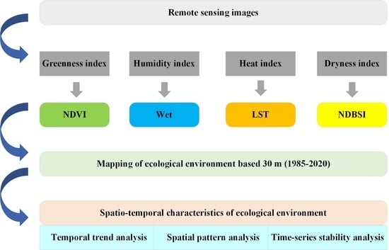
2.2. Calculation of Remote Sensing-Based Ecological Index

2.2.1. Calculation of Ecological Index

Xu Hanqiu [45] combined four parameters closely related to the natural ecological environment to construct a remote sensing-based ecological index, namely greenness, humidity, heat, and dryness. The meanings and methods of calculating of each ecological factor used in the index are described below.
(1)
Greenness index
Vegetation is an extremely important factor that reflects the quality of the ecological environment in a region. The greenness indicator was expressed by the normalized difference vegetation index (NDVI), which could represent the growth status of plants, the distribution of the vegetation density, and the coverage of vegetation [67]. The formula was defined as follows:
N D V I = ρ N I R ρ R / ρ N I R + ρ R
where ρNIR is the reflectance of the near-infrared band in remote sensing data, and ρR is the reflectance of the infrared band in remote sensing data. In Landsat 8 data, they corresponded to the 5th and 4th bands, respectively. In Landsat 5 data, they corresponded to the 4th and 3rd bands, respectively.
(2)
Humidity index
The humidity can reflect the moisture content of vegetation and soil [68,69,70]. In this study, the humidity component in the tasseled cap transformation was used instead of the humidity index, being denoted as tasseled cap wet. The formulas used to calculate the humidity index based on Landsat TM/OLI images was as follows:
W e t T M = 0.0315 ρ B + 0.2021 ρ G + 0.3102 ρ R + 0.1594 ρ N I R 0.6806 ρ S W I R 1 0.6109 ρ S W I R 2
W e t O L I = 0.1511 ρ B + 0.1972 ρ G + 0.3283 ρ R + 0.3407 ρ N I R 0.7117 ρ S W I R 1 0.4559 ρ S W I R 2
where WetTM is the humidity result obtained using the Landsat 5 satellite data, and WETOLI is the humidity result obtained using Landsat 8 satellite data. ρB, ρG, ρR, ρNIR, ρSWR1, and ρSWR2 are the reflectances of the blue, green, red, near-infrared, shortwave infrared 1, and shortwave infrared 2 bands, respectively.
(3)
Dryness index
Soil drying caused by developed land and bare soil can seriously harm the ecological environment in a region. In this study, the NDBSI, which reflected the degree of soil drying, was calculated by combining an index-based built-up index (IBI) and a normalized bare soil index (SI) [71]. The formula used was as follows:
N D B S I = I B I + S I / 2
where IBI and SI are the index-based built-up index and normalized bare soil index, respectively. The specific formulas used to calculate these indices were as follows:
I B I = 2 ρ S W I R 1 / ρ S W I R 1 + ρ N I R ρ N I R / ρ N I R + ρ R + ρ G / ρ S W I R 1 + ρ G 2 ρ S W I R 1 / ρ S W I R 1 + ρ N I R + ρ N I R / ρ N I R + ρ R + ρ G / ρ S W I R 1 + ρ G
S I = ρ S W I R 1 + ρ R ρ N I R + ρ B / ρ S W I R 1 + ρ R + ρ N I R + ρ B
where ρB, ρG, ρR, ρNIR, ρSWR1, and ρSWR2 are the reflectances of the blue, green, red, near-infrared, shortwave infrared 1, and shortwave infrared 2 bands, respectively.
(4)
Heat index
The LST is an important component of the Earth’s energy budget and an important parameter representing the surface environment. In this study, the obtained LST was used to represent the heat index. Regarding the Landsat series of satellites, Landsat 5 has one thermal infrared band (band 6, 10.40–12.50 μm), and the TIRS sensor on the Landsat 8 has two thermal infrared bands (band 10, 10.60–11.19 μm; band 11, 11.50–12.51 μm). Band 10 is located in a lower atmospheric absorption region than band 11 and has a higher atmospheric transmission accuracy. Therefore, band 6 of Landsat 5 and band 10 of Landsat 8 were selected as the channels used to perform the LST inversion.
The statistical mono-window model (SWM) was used to invert the LST [72]. The calculation of the land surface emissivity adopted the vegetation cover method [73], and the fractional vegetation cover was calculated using the NDVI. The specific formulas used to calculate the SWM were as follows:
L 6 = g a i n × D N + b i a s
T b = K 2 / ln K 1 / L 6 + 1
p v = N D V I N D V I m i n / N D V I m a x N D V I m i n 2
ε = 0.004 × p v + 0.986
L S T = T b / 1 + λ T b / ρ ln ε 273.15
where L6 is the radiance-calibrated thermal infrared band reflectance, and Tb is the temperature value at the sensor. DN is the gray value of the data pixel, and gain and bias are the band gain value and bias values, respectively, which can be obtained using the image header. K1 and K2 are calibration parameters, which can be obtained by referring to the user manual (for Landsat 5, K1 = 607.76 W × m−2 × um−1 × sr−1 and K2 = 1260.56 K; for Landsat 8, K1 = 774.89 W × m−2 × um−1 × sr−1 and K2 = 1321.08 K). ε is the land surface emissivity, which was calculated by applying a threshold to the NDVI according to Sobrino’s method [74]. pv is the fractional vegetation cover, NDVI is the normalized difference vegetation index, and NDVImin is the minimum value of the NDVI, which represents the NDVI value of completely bare soil or areas with no vegetation cover. NDVImax is the maximum value of the NDVI, which represents the NDVI value of pure vegetation pixels. LST is the land surface temperature, and ρ = 1.438 × 10⁻² mK. λ is the center wavelength of the thermal infrared band, where λTM = 11.435 μm and λTIR1 = 10.900 μm [75].

2.2.2. Construction of RSEI

Using remote sensing technology to calculate the vegetation index, humidity component, LSY, and NDBSI, which represent the greenness, humidity, heat, and dryness, respectively, and are closely related to the surface ecological environment, the RSEI was constructed. The specific formula used to calculate the RSEI was as follows:
R S E I = f N D V I , W e t , L S T , N D B S I
where NDVI, Wet, LST, and NDBSI represent the normalized difference vegetation index, humidity component obtained via the tasseled cap transformation, the land surface temperature, and the normalized difference bare soil index, respectively. f is the RSEI as a function of these four indexes, and in this paper, principal component analysis (PCA) was used to integrate these four ecological indexes.
PCA is a multidimensional data compression technique that uses orthogonally rotated coordinate axes and linear transformations to condense information derived from multiple variables into a few characteristic components [76]. Using this method to synthesize multiple indicators can avoid the bias caused by subjective factors in the weighting process and ensure the representativeness of the obtained principal components [77]. To avoid imbalance in weights caused by non-standardized units, the ecological factors were normalized to the range of (0–1) before performing PCA, and the formula used in normalization iwass as follows:
N I i = I i I m i n / I m a x I m i n
where NIi is the result of normalized processing of the index, and Ii, Imin, and Imax are the values of the ith pixel of the index, the minimum value, and the maximum value, respectively.
Based on the results of the PCA, the first component, i.e., PC1, integrated the various ecological factors and contained information about the vast majority of the ecological indexes, meaning that it could be used to characterize the quality of the ecological environment of the ground corresponding to the pixel. To ensure that a higher PC1 value represented a better ecological condition, we could obtain the initial ecological index RSEI0 [78] by subtracting PC1 from Equation (1). The formula is as follows:
R S E I 0 = 1 P C 1 f N D V I , W e t , L S T , N D B S I
To facilitate measurement and comparison of the indices, RSEI0 was normalized as follows:
R S E I f = R S E I 0 R S E I 0 _ min / R S E I 0 _ max R S E I 0 _ min
where RSEIf is the remote sensing-based ecological index constructed, and its value ranges from 0 to 1. The closer the RSEI value was to 1, the better the ecological condition; the closer the value was to 0, the worse the ecological condition [79].

2.3. Analysis of Spatiotemporal Patterns of Ecological Environment Based on RSEI

2.3.1. Analysis of Ecological Environment Grading and Conversion Based on RSEI

In this study, the RSEI was divided into five levels with an interval of 0.2 based on the Technical Guidelines for Ecological Environment Evaluation (HJ/T 192-2015) published in 2015: poor (0–0.2], relatively poor (0.2–0.4], general (0.4–0.6], good (0.6–0.8], and excellent (0.8–1]. The ecological environmental quality of the Zhoushan Archipelago was analyzed at five-year intervals from 1985 to 2020. The ArcGIS raster reclassification tool was used to classify the ecological environmental quality of the study area into five levels, creating a spatial distribution map of the ecological environmental quality in the Zhoushan Archipelago. The proportion of the areas occupied by each level of ecological environmental quality and the total area were then calculated. Finally, two RSEI grading maps at five-year intervals were overlain to generate the ecological environment grading transition matrix. Based on this matrix, the ecological environment grading transition Sankey diagram was generated.

2.3.2. Analysis of Ecological Environment Change Trend

Trend analysis compared the same indicators or ratios recorded in different time periods, directly observed their changes and magnitudes, examined their development trends, and predicted their future development prospects [80]. In the time-series trend analysis, the Mann–Kendall (M–K) test was combined with the Theil–Sen median trend analysis method to analyze the change trend of the ecological environment in the study area from 1985 to 2020.
The Mann–Kendall test is a non-parametric statistical test method used to determine the significance of trends. It does not require the sample to follow a certain distribution and is not affected by a few outliers [81]. The computational formula used to perform the Mann–Kendall test was as follows:
Set {RSEIi}, i = 1985, 1990,…, 2015, 2020.
The Z statistic was defined as follows:
Z = S 1 s S , S > 0 0 , S = 0 S + 1 s S , S < 0 ,   S = j = 1 n 1 i = j + 1 n sgn R S E I j R S E I i
sgn R S E I j R S E I i = 1 , R S E I j R S E I i > 0 0 , R S E I j R S E I i = 0 1 , R S E I j R S E I i < 0 ,   s S = n n 1 2 n + 5 18
where RSEIi and RSEIj are the RSEI values of pixel i in year i and year j, respectively; n is the length of the time series; and sgn is the sign function. The value range of the Z statistic is the real set R. At the given significance level α, when | Z | > μ 1 2 , there was a significant change in the research sequence at level α [82]. In this paper, α was set at 0.05 to determine the significance of the RSEI time-series trend at a confidence level of 0.05.
Theil–Sen median trend analysis is a robust non-parametric method used to calculate trends that can reduce the influence of data outliers [83]. The Theil–Sen median trend analysis method calculates the median of the slope of n(n − 1)/2 combinations of data. The computational formula used was defined as follows:
S R S E I = M e d i a n R S E I j R S E I i j i ,   1985 i < j 2020
when SRSEI > 0, the RSEI time series exhibited an increasing trend, and when SRSEI < 0, the RSEI time series exhibited a decreasing trend.

2.3.3. Analysis of Ecological Environmental Change Sustainability

Sustainability analysis predicts future trends based on existing changes. In this study, the sustainability of the ecological environment time-series change was analyzed based on the Hurst index. The Hurst index, which is also known as the index dependency or index long-term dependence, can quantify the relative trend of a time series. Rescaled range (R/S) analysis was first proposed by Hurst (1951) for the analysis of hydrological data for the Nile and has subsequently been developed. Among the many algorithms used to estimating the Hurst index, the most famous example is the R/S method used by Mandelbrot and Wallis based on Hurst’s hydraulic research results [84]. The R/S method is used to analyze long-term time-series correlations and has wide applications in hydrology, economics, climatology, geology, and geochemistry [85]. Its basic principle is as follows [86].
For a time series {RSEI(t)}, t = 1, 2, …, n, the mean series was defined as follows:
R S E I ¯ ( τ ) = 1 τ t = 1 τ R S E I ( τ ) ,   τ = 1 ,   2 ,   ,   n .
The formula for cumulative deviation was
X ( t , τ ) = t = 1 t R S E I ( t ) R S E I ( τ ) ¯ ,   1 t τ
The formula for the range sequence was
R ( τ ) = max 1 s t s τ X ( t , τ ) min 1 s t s τ X ( t , τ ) ,   τ = 1 ,   2 ,   ,   n
The formula for the standard deviation sequence was
S ( τ ) = 1 τ t = 1 τ R S E I ( t ) R S E I ( τ ) 2 1 2 ,   τ = 1 ,     2 ,   ,   n
By taking the ratio of R(τ) to S(τ), we obtained
R / S = R ( τ ) / S ( τ )
R / S τ 2 H
The Hurst exponent, which was denoted as H, ranged from 0 to 1 and characterized the existence of the Hurst phenomenon in a time series. The value of H was used to determine whether the RSEI sequence was completely random or exhibited persistence based on the following three scenarios: (1) When H > 0.5, the process exhibits sustainable properties, that is, the future trend is consistent with the past trend, and the stronger the persistence is, the closer H is to 1. (2) When H = 0.5, the RSEI time series is a random sequence, without long-term correlation. (3) When H < 0.5, the time series exhibits non-sustainability, and the stronger the non-sustainability, the closer H is to 0 [87].

2.3.4. Temporal Stability Analysis of the Ecological Environment

The coefficient of variation is the ratio of the standard deviation to the mean of the original data, reflecting the absolute degree of dispersion of the data. A larger value indicates a more dispersed data distribution and greater inter-annual fluctuations. Conversely, a smaller value indicates a more concentrated data distribution, smaller inter-annual fluctuations, and a greater temporal stability in the time series. By calculating the coefficient of variation in the RSEI in the Zhoushan Archipelago, we determined the degree of dispersion of the RSEI values in the study area and the stability of the long-term RSEI time series. The calculation formula used was as follows [88]:
C V = 1 n i = 1 n R S E I i 1 n i = 1 n R S E I i 1 n i = 1 n R S E I i
where CV is the coefficient of variation, n is the number of years, i is the year index, and RSEIi is the remote sensing-based ecological index of the ith year.

3. Study Area and Data Sources

3.1. Study Area

The Zhoushan Archipelago is located on the coast of the East China Sea and bordered by Hangzhou Bay to the west, Shanghai to the north, and Ningbo to the south (Figure 2). It serves as a significant geographic gateway to the Yangtze River Basin and the Yangtze River Delta [89]. Geographically, the Zhoushan Archipelago is characterized by a low hilly landscape, with approximately 37.4% of the terrain consisting of hills, and a complex distribution of water systems, including underdeveloped surface water systems [65]. It has a subtropical monsoon humid climate, having a moderate climate throughout the year, distinct seasons, warm winters, and cool summers. The average annual temperature is 16 °C. The vegetation in the archipelago is dominated by evergreen broad-leaved forests in the Chinese subtropical region, which primarily consist of mixed forests of broad-leaved trees and shrubs [90]. Additionally, the archipelago is home to abundant biological resources and plays an important role as a habitat for island-dwelling birds.
Zhoushan City was the first prefecture-level city to be established in island form in China, covering a total of 2085 islands, representing 20% of China’s islands [91]. Moreover Zhoushan Island is the largest in the Zhoushan Archipelago and the third largest in the country. It is home to 74% of the total population of Zhoushan City and serves as the administrative and economic center of the urban area located in the Zhoushan Archipelago [92]. Due to the unique geographic location of the islands, the fragile ecological environment in the Zhoushan Archipelago is susceptible to frequent interactions between land, sea, atmosphere, human activities, natural disasters, intensified urbanization, and global climate change [93].

3.2. Data Sources

In this study, Landsat series satellite images were used. The Landsat series is one of the longest-operating optical remote sensing satellite systems and has the advantages of a long time series, high spatial resolution, and high data availability [94,95]. Since the 1970s, a total of nine Landsat satellites have been launched, all of which have successfully acquired a substantial amount of Earth observation data, except for Landsat 6, which failed to launch [96,97]. The latest Landsat satellite, known as Landsat 9, was launched in September 2021 [98,99]. It will continue to provide long-term data products, achieve the goal of continuously monitoring land surface landscape changes in the Landsat plan, and continue the long-term Landsat observation record [100,101]. Currently, the Landsat series has become an important information source for the long-term monitoring of land use and land cover changes and the ecological environments of Earth [102,103,104].
In this study, surface reflectance (SR) data from Landsat 5 thematic mapper (TM) sensors for the years 1985, 1990, 1995, 2000, 2005, and 2010 and Landsat 8 operational land imager/thermal infrared sensor (OLI/TIRS) for 2015 and 2020 were selected through the GEE cloud-based platform. Landsat images acquired during the growing sensor (from May to October) were selected, and we proposed annual composite images using median values to ensure the seasonal consistency of the temporal analysis. The cloud and shadow mask algorithm on the GEE cloud-based platform was then applied to remove clouds and shadows from the obtained images, achieving the goal of eliminating anomalous values and improving the image quality. The data used in this study are described in Table 1.

4. Results and Analysis

4.1. RSEI Calculation for the Zhoushan Archipelago

Based on satellite remote sensing data used to characterize ecological environmental factors, such as greenness, humidity, temperature, and dryness, the RSEI was calculated using PCA. The results of the PCA for the study area from 1985 to 2020 are presented in Table 2, with the analyzed indicator values of the first to fourth principal components denoted as PC1, PC2, PC3, and PC4, respectively.
As can be seen in Table 2, (1) the contribution rates of the four indicators to the first principal component exceeded 65% in all years, with values of 67.95%, 66.54%, 66.61%, 74.10%, 74.14%, 77.71%, 89.94%, and 88.25% recorded in 1985, 1990, 1995, 2000, 2005, 2010, 2015, and 2020, respectively. (2) Compared to the other components, the first principal component concentrated over 65% of the characteristic information of each indicator and could integrate the information of each indicator well, representing the ecological environmental characteristics of the region. Therefore, it was used to construct the RSEI and characterize the ecological environmental status of the region.
Based on the calculation results of the remote sensing-based ecological index for each year of the study period, a spatial distribution map of the RSEI with a 30-meter resolution for the Zhoushan Archipelago from 1985 to 2020 was generated (Figure 3).
As can be seen in Figure 3, the range of the remote sensing-based ecological index values from 1985 to 2020 in the Zhoushan Archipelago was 0–1. The areas with relatively high RSEI values were mainly located in the interior regions of the major islands in the archipelago, while the areas with relatively low RSEI values were mainly distributed in the eastern part of Zhoushan Island, the southwestern part of Jintang Island, the northern part of Daishan Island, the southern part of Qushan Island, the northern and northwestern parts of Zhujiajian, and the northwestern and eastern parts of Liuheng Island. To quantitatively analyze the changes in the RSEI during the study period, the mean and standard deviation of the RSEI and the four component indexes for each year were calculated, and a line graph recording the changes in the remote sensing-based ecological index in the Zhoushan Archipelago from 1985 to 2020 was created. The results are presented in Table 3 and Figure 4.
As can be seen in Table 3 and Figure 4, the overall ecological environment of the Zhoushan Archipelago was good from 1985 to 2020, but the mean RSEI exhibited a decreasing trend over time. The mean RSEI decreased from 0.7719 in 1985 to 0.7566 in 2000, and it further decreased to 0.5817 in 2020. This declining trend indicates that the ecological environment of the Zhoushan Archipelago has deteriorated by approximately 25% in the past 35 years. The decline was relatively slow from 1985 to 2000, though it was more severe from 2000 to 2020. During the study period, the standard deviation of the RSEI was relatively small, indicating that the data concentration was high, and the research results were more reliable.

4.2. Spatial Pattern Analysis of the Ecological Environmental Evolution

4.2.1. Rank Division of Ecological Environment

To better analyze the changes in the ecological environment of the Zhoushan Archipelago, it was necessary to rank the RSEI. Referring to the Technical Specification for the Evaluation of Ecological Environment Status (HJ/T 192-2015) issued in 2015, the ecological environment levels were classified using an interval of 0.2 as follows: poor (0–0.2], relatively poor (0.2–0.4], general (0.4–0.6], good (0.6–0.8], and excellent (0.8–1] (Table 4 and Figure 5).
Table 4 and Figure 5 show the area in of the ecological environment levels in the Zhoushan Archipelago from 1985 to 2020. The statistical results show that the proportion of areas with excellent ecological environments decreased by 38.83%, while the proportion of areas with poor ecological environments increased by 8.53%. Therefore, the ecological environment of the Zhoushan Archipelago exhibited an overall decreasing trend. The specific analysis is as follows: (1) From 1985 to 2020, the ecological environment of the Zhoushan Archipelago was mainly at the excellent level, having an average of 49.80% per year, but the proportion of the excellent areas decreased over time. Indeed, the proportion of the excellent ecological environment was highest in 1985, accounting for 67.46% of the total area, and it was lowest in 2020, accounting for 28.63% of the total area. (2) From 1985 to 2020, the proportion of areas with good ecological environments in the Zhoushan Archipelago was second only to those with excellent ecological environments. Except for 1985, it exceeded one-fifth of the total area, having an average of 24.21%. Indeed, the proportion of areas with good ecological environments was highest in 2010, accounting for 33.73%, while it was lowest in 1985, accounting for 16.46%. (3) From 1985 to 2020, the proportion of areas with a general ecological environment in the Zhoushan Archipelago ranked third, having an average of 12.17%. Indeed, the proportion of areas with general ecological environments was highest in 2020, accounting for 16.68%, while it was lowest in 1990, accounting for 7.25%. (4) From 1985 to 2020, the proportions of areas with poor and relatively poor ecological environments in the Zhoushan Archipelago were relatively small, having averages of 4.60% and 9.22%, respectively. Except for 2015 and 2020, the sum of the areas with these two levels was less than 16% in all years, but their overall proportions exhibited an increasing trend. Indeed, the sum of the areas with poor and relatively poor ecological environments was highest in 2020, accounting for 27.67% of the total area. The sum of the areas with poor and relatively poor ecological environments was smallest in 1985 and 2000, accounting for 7.64% and 7.62% of the total area, respectively.

4.2.2. Level of Conversion of Ecological Environment

In order to further analyze the spatiotemporal changes in the ecological environment of the Zhoushan Archipelago, the classified RSEI results for each study period were overlaid, and a Sankey diagram (Figure 6) and an ecological environment level transition matrix (Figure 7) were created to illustrate the results.
The Sankey diagram clearly describes the direction and volume of the changes in the ecological environment levels, which quantitatively expresses the transition relationship between the ecological environment levels during different periods. It can be concluded based on Figure 6 that the characteristics of the ecological environment level conversions every 5 years can be summarized as follows: the transition between every two adjacent levels was relatively drastic. In particular, the transitions between excellent and good, good and general, general and relatively poor, and relatively poor and poor ecological environments were significant transitions.
The ecological environment level transfer matrix visually reflects the specific areas in which ecological environment level changes occurred, and it has great significance for quantifying the transitions between different ecological environment levels in each period. In this study, the ecological environment level transfer matrix was created every 5 years from 1985 to 2020 (Figure 7). It can be concluded based on Figure 7 that there were significant changes in the ecological environment levels in the Zhoushan Archipelago from 1985 to 2020. (1) During the study period, the conversion from the excellent to the good level was dominant, with the largest period of conversion occurring from 2010 to 2015, during which time 131.3087 km2 were converted from the excellent to the good level. The main category converted to the excellent level was the good level, with a maximum conversion area of 186.8389 km2 (2005–2010). (2) The main category converted from the good level was the excellent level, followed by the conversion from the good to the general levels. The maximum area converted from the good to the general level was 33.8996 km2 (2015–2020), and the maximum area converted from the general to the good level was 79.0286 km2 (2010–2015). (3) The main areas converted from the general level was converted to the good and relatively poor levels. The maximum area converted from the relatively poor to the general level was 83.2385 km2 (2010–2015), and the maximum area converted from the general to the relatively poor level was 37.2699 km2 (2015–2020). (4) Except for the conversion between the general and relatively poor levels, the conversion from and to of the relatively poor level mainly occurred with regard to the poor levels. The maximum area converted from the poor to the relatively poor level was 97.3449 km2 (2010–2015), and the maximum area converted from the relatively poor to the poor level was 36.3026 km2 (2015–2020). (5) Aside from the conversion of the very poor level, the amount of area converted from the poor level to other levels was relatively small, with the minimum conversion amount occurring during the period 1995–2000, during which time the area converted to the good level was only 0.0047 km2. The conversion to the poor level mainly occurred from the relatively poor and general levels, and the maximum area converted from the general to the poor level was 11.6758 km2 (2015–2020).

4.3. Temporal Trend Analysis of Ecological Environmental Evolution

4.3.1. Change Trend of Ecological Environment

By combining Theil–Sen median trend analysis and the Mann–Kendall test, we effectively analyzed the change trend and spatial distribution characteristics of the ecological environment in the Zhoushan Archipelago from 1985 to 2020. Since there were basically no regions with SRSEI values strictly equal to 0 in this study, the regions with SRSEI values of −0.0005 to 0.0005 were defined as regions with stable and unchanged ecological environments, regions with SRSEI values of greater than 0.0005 were defined as regions with an improved ecological environment, and regions with SRSEI values of less than −0.0005 were defined as regions with a degraded ecological environment, thus dividing the ecological environmental changes in the study area into three different categories. In the significance analysis, after setting the significance level at 0.05, the significance of the RSEI time-series trend change was assessed. The results of the significance test were divided into significant changes (Z > 1.96 or Z < −1.96) and slight changes (−1.96 ≤ Z ≤ 1.96). The results of the Theil–Sen median trend analysis and the Mann–Kendall test were superimposed to obtain the RSEI change trend results at the pixel scale from 1985 to 2020. The results were divided into five types of change (Table 5).
As can be seen in Table 5, the area with an improved ecological environment accounted for 12.60% of the total area, the stable and unchanged ecological environment areas accounted for 3.05% of the total area, and the areas with a degraded ecological environment accounted for 84.35% of the total area. Therefore, most of the areas in the Zhoushan Archipelago exhibited a trend of ecological environmental degradation from 1985 to 2020. Indeed, 50.25% of the study area had a slightly degraded ecological environment, while 34.10% of the area had a seriously degraded ecological environment. The proportion of the areas with significant improvement in the ecological environment was the smallest, accounting for only 0.84% of the total area.
As can be seen in Figure 8, the area of ecological environment degradation in the Zhoushan Archipelago far exceeded the area of ecological environment improvement from 1985 to 2020. The areas with significantly degraded ecological environments were mainly located in the southern part of Zhoushan Island, the southwestern part of Jintang Island, the northwestern area of Zhujiajian Island, the northern area of Taohua Island, the central part of Liuheng Island, and the western parts of Qushan Island, Shengsi Island, and Yangshan Island. The areas with slightly degraded ecological environments were mainly located in the central part of Zhoushan Island, the eastern parts of Jintang Island and Zhujiajian Island, and the southern parts of Dachangtu Island and Yushan Island. The areas with stable ecological environments were scattered throughout the archipelago. The areas with slightly improved ecological environments were mainly located in the northeastern and eastern parts of Zhoushan Island, the southern parts of Taohua Island and Zhujiajian Island, the southwestern area of Liuheng Island, and the northern area of Qushan Island. The areas with significantly improved ecological environments were scattered within the inner areas of the slightly improved areas.

4.3.2. Sustainability Analysis of Ecological Environment

The Hurst exponent was used to explore the sustainability of the change trends of the ecological environment of the Zhoushan Archipelago. The results show that the average Hurst index of the RSEI is 0.65, with the areas in which the Hurst index is less than 0.5 accounting for 13.39% of the total area and the areas in which it is greater than 0.5 accounting for 86.61% of the total area. These results indicate that the ecological environmental changes in the Zhoushan Archipelago have a strong positive persistence, meaning it will have a strong tendency to continue its original change trend in the future.
The Theil–Sen median trend analysis quantitatively reflects the change trend of the RSEI during a given period, while the Hurst exponent qualitatively predicts whether the change trend is sustainable. The sustainability of the RSEI changes in the Zhoushan Archipelago is obtained by superimposing the results of the RSEI change trend on the Hurst exponent results. In this paper, the results are categorized into four levels (Table 6 and Figure 9).
As can be seen in Table 6 and Figure 9, in most areas of the Zhoushan Archipelago, the ecological environment exhibited a trend of degraded sustainably, having an area proportion of 73.40%. The regions in which the ecological environment exhibited a trend of sustainably stability accounted for 2.65% of the total area, and these regions were scattered in the central part of Zhoushan Island and the western part of Taohua Island. The regions in which the ecological environment exhibited a trend of improved sustainably accounted for 10.56% of the total area and were mainly located in the eastern and northeastern parts of Zhoushan Island; the northern, northwestern, and southern parts of Zhujiajian Island; the southern part of Taohua Island; the southwestern part of Liuheng Island; the northern part of Yangshan Island; and the southern and northern parts of Qushan Island. The area proportion in which the trend of the change was unsustainable was 13.39%, and these areas were scattered within the central areas of the islands, such as the central parts of Zhoushan island. In conclusion, the protection of the ecosystem in the Zhoushan Archipelago should be given due attention. In particular, the regions with a sustainable degradation trend require special attention.

4.4. Time-Series Stability Analysis of Ecological Environmental Evolution

To determine the time-series stability of the ecological environmental changes in the Zhoushan Archipelago recorded in this study, the coefficient of variation in the RSEI from 1985 to 2020 was calculated. The coefficient of variation values for each pixel were then counted and used to create a cumulative frequency graph (Figure 10).
As can be seen in Figure 10, the coefficient of variation was mainly concentrated between 0 and 0.4, having an average value of 0.1627 and a standard deviation of 0.1467. The pixels with a coefficient of variation of 0.04 had the largest number of occurrences, having a frequency of nearly 350,000. The second largest frequency was for pixels with a coefficient of variation of 0.06, which had a frequency of greater than 250,000. This result indicates that the RSEI values in the Zhoushan Archipelago were relatively concentrated between 1985 and 2020, with small inter-annual fluctuations and a relatively stable time series.
According to Jenks [105], there are natural breakpoints and turning points in any data series, which are statistically significant and can be used to divide the research object into groups with similar properties. Therefore, natural breakpoints are good boundaries for classification. The natural breaks method is a method of classifying data based on natural breakpoints. It determines the best arrangement of values in a group by iteratively comparing the sum of squares of the differences between each grouping and the mean of the elements in the grouping to the observed values. Based on the calculated best arrangement, the cutoff points present in an ordered distribution are determined, and the elements are divided into multiple categories by setting boundaries at the cutoff points. This classification method can minimize the sum of the squared differences between groups, maximize the variance between groups, and minimize the variance within groups, achieving the goal of classification.
To explore the time-series stability of the ecological environmental changes in the study area, the coefficient of variation results were classified into five categories using the natural breaks method: very stable (0 < CV ≤ 0.10), relatively stable (0.10 < CV ≤ 0.21), slightly variable (0.21 < CV ≤ 0.33), moderately variable (0.33 < CV ≤ 0.48), and highly variable (0.48 < CV ≤ 1.0). The spatial distribution of the coefficient of variation values is shown in Table 7 and Figure 11.
As can be seen in Table 7 and Figure 11, there are spatial differences in the time-series stability of the ecological environment changes. The areas with moderately variable and highly variable coefficients of variation account for a small proportion of the total area, i.e., 11.22% and 4.52%, respectively. These areas are mainly located in the northeastern part of Zhoushan Island, the northern part of Daishan Island, the southern and northern areas of Yangshan Island, the edges of Liuheng Island, the western area of Zhujiajian Island, and the northwestern, northeastern, and southwestern parts of Jintang Island. These coastal areas are relatively flat and greatly affected by natural disasters and human activities, leading to large fluctuations in the RSEI values. The areas that are very stable and relatively stable account for a large proportion of the total area, i.e., 49.40% and 19.25%, respectively. These areas are mainly located in the central areas of the major islands, such as the central areas of Zhoushan Island, Daishan Island, Liuheng Island, Taohua Island, Jintang Island, Xiushan Island, Qushan Island, and Changtu Island, as well as the small islands that have not been developed and utilized by humans. These areas have a high vegetation cover and are less affected by natural phenomena and human activities, maintaining good ecological conditions, thus resulting in small overall fluctuations and a stable time-series of RSEI values over time. The areas classified as slightly variable accounted for 15.61% of the total area and were mainly distributed in the transition zone between the relatively stable and moderately variable regions.

5. Discussion

In this study, long-term time-series Landsat satellite remote sensing data provided by the GEE platform were utilized to efficiently monitor and assess the ecological environment of the Zhoushan Archipelago, and the spatiotemporal variations were comprehensively investigated. Although the experimental results exhibit some degree of effectiveness, uncertainties also exist in the findings.

5.1. Rationality of Mapping of Ecological Environment of Islands Using Remote Sensing Images

Remote sensing is a technique used to monitor the Earth’s surface from a distance, and the acquired remote sensing images can be applied through interpretation, analysis, and visualization [106,107,108]. Compared to other conventional methods, this method has several significant advantages. Firstly, remote sensing technology provides abundant information with a short information acquisition cycle, meaning that it is a rich data source for long-term ecological environment monitoring. Based on the Landsat satellite remote sensing data derived from 1985 to 2020 and integrated into the GEE cloud-based platform, an RSEI model was constructed to monitor and evaluate the ecological environment of the Zhoushan Archipelago. This model accurately detected the characteristics of the ecological environmental changes, and the results provided technical support for the formulation of regional ecological environment monitoring and development planning strategies. Secondly, remote sensing technology can achieve large-scale, long-term, and continuous observation at fixed points, making it more efficient than other traditional methods [109,110]. Based on the remote sensing technology, powerful online visualization calculation ability, and cloud storage characteristics of the GEE cloud platform [111,112,113,114], in this study, the quality of the regional ecological environment was objectively and rapidly evaluated by obtaining indicators closely related to the ecological environmental quality, such as greenness, humidity, dryness, and heat. Thirdly, remote sensing technology is characterized by comprehensiveness and can form a widely distributed detection network while observing the temporal, spatial, and spectral characteristics of objects, thereby obtaining true geographic information about objects within the regional space [115]. Compared to social statistical yearbook data, it can reflect the geographic distribution characteristics and relationships between things. For example, the ecological environment grading map created in this study based on remote sensing data reflects the spatial distribution characteristics of the different ecological environment levels in the Zhoushan Archipelago and lays the foundations for subsequent analysis of the spatiotemporal evolution of the ecological environment.

5.2. Uncertainties of Mapping of Ecological Environment of Islands Using Remote Sensing Images

Remote sensing technology can quickly monitor the ecological environment status of a region, but some factors affect the accuracy of ecological environment assessment. From the perspective of the inherent defects of remote sensing technology, the spatial resolution determines the size of the pixels covering the Earth’s surface in satellite images, and the RSEI represents the ecological environmental status of the ground covered by the pixel [116]. However, the mixed pixels in the remote sensing images create certain differences between the acquired information and the true values, which may cause some uncertainties regarding the calculation of the RSEI [117,118]. In some areas of the Zhoushan Archipelago, the vegetation cover is high, and the NDVI value may be saturated, which may lead to the inaccurate calculation of the greenness index. In the future, the leaf area index (LAI) will be used instead of the NDVI to invert the greenness index of the remote sensing-based ecological index [119,120,121]. As developed land is often covered by impermeable surfaces, such as building roofs, paved roads, and parking lots [122,123,124], the normalized difference impervious surface index (NDISI) can enhance the characteristics of the soil and developed land that cause dry land surfaces compared to the NDBSI. Therefore, the NDISI can be used instead of the NDBSI to invert the dryness index and make the results more accurate.

5.3. Prospects of Remote Sensing Technology for Ecological Environmental Monitoring

Remote sensing data have become important sources of information used to study surface conditions and monitor ecological environments. In recent years, with the development of remote sensing technology to include multiple platforms, sensors, and angles; higher spatial and spectral resolutions; and quantitative remote sensing in practical applications, remote sensing technology is playing an increasingly important role in ecological environmental monitoring. On one hand, the combination of satellite remote sensing data and measured data can improve the accuracy of ecological environmental remote sensing monitoring. On the other hand, the fusion of space–time technology has the ability to enhance image quality, obtain temporal remote sensing data that can be used to describe the ecological conditions in different periods, and reveal the evolutionary characteristics of the ecological environment at the fine scale [125,126,127,128]. Moreover, new techniques, such as cloud computing, big data, and artificial intelligence, have injected new vitality into remote sensing image processing and provide innovative technical means of solving the large-scale automatic processing of and intelligent information extraction from satellite data, which can fully tap the value of massive remote sensing data and promote the rapid development of remote sensing technology [129,130,131].

6. Conclusions

Based on the GEE cloud-based platform and Landsat satellite remote sensing data, in this study, the NDVI, Wet, LST, and NDBSI were selected to characterize the closely related greenness, humidity, heat, and dryness of the ecological environment, respectively. The RSEI was constructed using PCA, and RSEI distribution maps with 30-meter spatial resolutions for eight time periods from 1985 to 2020 in the Zhoushan Archipelago were created. The trends and patterns of the spatiotemporal evolution of the ecological environment in the Zhoushan Archipelago were explored using the Theil–Sen median trend analysis, Mann–Kendall test, Hurst index, and coefficient of variation method. The spatial pattern, temporal trend, and temporal stability of ecological environmental evolution in the Zhoushan Archipelago from 1985 to 2020 were clarified. The main conclusions are as follows:
(1)
The average RSEI values for the eight time periods (at five-year intervals) from 1985 to 2020 were 0.7719, 0.7532, 0.7657, 0.7566, 0.7293, 0.6682, 0.6250, and 0.5817. Except for 2020, the RSEI values for all years were within the range 0.6–0.8. During the entire study period, the average RSEI value in the Zhoushan Archipelago decreased from 0.7719 to 0.5817, indicating an overall declining trend regarding the ecological environment in the study area.
(2)
The area change in each ecological environment level was obvious in the Zhoushan Archipelago during the study period. From 1985 to 2020, the proportion of areas with an ecological environment grade of excellent decreased by 38.83%, while the proportion of areas with ecological environment grades of poor and relatively poor increased by a total of 20.03%. The proportions of areas with ecological environment grades of good and general increased by 10.56% and 8.24%, respectively. Based on the results of the ecological environment grade conversion, the transition between each pair of adjacent grades was relatively drastic. The transition between the excellent and good grades was dominant, with the largest area of transition from the excellent to the good grade occurring from 2010 to 2015, covering an area of 131.3087 km2. The largest area of transition from good to excellent grade was 186.8389 km2, occurring from 2005 to 2010. The good and general grades exhibited the second largest transition areas. During the study period, the largest area of transition from general to good grade was 79.0286 km2, occurring from 2010 to 2015.
(3)
The ecological environment in the Zhoushan Archipelago exhibited co-existing degradation and partial improvement, with the areas with a degraded ecological environment accounting for 84.35% of the total area and the areas with an improved ecological environment accounting for 12.61% of the total area. The proportion of the areas with a significantly improved ecological environment was the smallest, accounting for only 0.84% of the total area. The proportion of the areas with a heavily degraded ecological environment was significant, accounting for 34.10% of the total area. These areas were mainly distributed in the southern part of Zhoushan Island, the southwestern part of Jintang Island, the northwestern area of Zhujiajian Island, the northern area of Taohua Island, the central part of Liuheng Island, and the western parts of Qushan Island, Shengsi Island, and Yangshan Island. The decline in the ecological environment in these areas was related to urbanization and the development of tourism resources in the Zhoushan Archipelago.
(4)
The results of the Hurst exponent analysis indicate that the change trend of the ecological environment in most regions of the Zhoushan Archipelago is sustainable. The proportion of the areas with degraded sustainably was 73.40%, and these areas were extensively distributed on the major islands in the Zhoushan Archipelago. The proportion of the areas with stable sustainably was 2.65%, and these areas were scattered in the central part of Zhoushan Island and the western part of Taohua Island. The proportion of the areas with improved sustainably was 10.56%, and these areas were mainly located in the eastern and northeastern parts of Zhoushan Island; the northern, northwestern, and southern parts of Zhujiajian Island; the southern part of Taohuajian Island; the southwestern part of Liuheng Island; and the northern part of Yangshan Island. The proportion of the unsustainable areas was 13.39%, and these areas were scattered within the central areas of the islands. In conclusion, the ecological environment in the areas with degraded sustainably requires particular attention.
(5)
The coefficient of variation in the RSEI sequence from 1985 to 2020 was mainly concentrated within the range 0–0.4, and its average value was 0.1627, indicating that the overall variations in the RSEI value in the Zhoushan Archipelago during the study period were relatively small, having a stable temporal trend. The regions with a high coefficient of variation were mainly concentrated in the northeastern part of Zhoushan Island, the northern part of Daishan Island, the edges of Liuheng Island, the western side of Zhujiajian Island, and the northwestern and southwestern parts of Jintang Island, indicating that the RSEI values in these areas fluctuated considerably over time.
The contributions of this study are that it provides a feasible method for ecological environmental monitoring in island areas, as well as data and technical support for the monitoring and evaluating of the regional ecological environment. However, this study only provides a simple description of the trend of the ecological environment in the Zhoushan Archipelago from 1985 to 2020, without offering specific analysis and discussion of the reasons and driving factors causing the changes. In the future, we will consider the relationship between the ecological environment and land use to better reveal the underlying causes of the ecological environment’s evolution. In addition, using data with longer time series and more dense time intervals to more accurately explore characteristics and trends will represent a follow-up work.

Author Contributions

Conceptualization, C.C. and G.Y.; methodology, C.C. and L.W.; formal analysis, C.C., L.W. and G.Y.; investigation, C.C. and W.S.; writing—original draft preparation, C.C. and L.W.; writing—review and editing, C.C., G.Y., W.S. and Y.S.; project administration, C.C.; funding acquisition, C.C., G.Y. and W.S. All authors have read and agreed to the published version of the manuscript.

Funding

This work was supported by the National Natural Science Foundation of China (Grant Nos. 42171311, 42271340, 41971296, and 42122009), in part by the Zhejiang Province Pioneering Soldier and Leading Goose R&D Project (Grant No. 2023C01027), in part by the Public Projects of Ningbo City (Grant No. 2021S089), and in part by the Ningbo Science and Technology Innovation 2025 Major Special Project (Grant Nos. 2021Z107 and 2022Z032).

Data Availability Statement

The data used in this paper are available from Google Earth Engine upon reasonable request, and the model, products, and codes generated in this paper are available from the corresponding author upon reasonable request.

Acknowledgments

The authors would like to thank the editors and the anonymous reviewers for providing outstanding comments and suggestions, which greatly helped to improve the technical quality and presentation of this manuscript. We thank LetPub (www.letpub.com, accessed on 9 July 2023) for providing linguistic assistance and pre-submission expert reviews.

Conflicts of Interest

The authors declare that they have no known competing interest that could have appeared to influence the work reported in this paper.

References

  1. Fan, Y.; Fang, C.; Zhang, Q. Coupling coordinated development between social economy and ecological environment in Chinese provincial capital cities-assessment and policy implications. J. Clean. Prod. 2019, 229, 289–298. [Google Scholar] [CrossRef]
  2. Zhang, Q.; Yin, Z.; Lu, X.; Gong, J.; Lei, Y.; Cai, B.; Cai, C.; Chai, Q.; Chen, H.; Dai, H.; et al. Synergetic roadmap of carbon neutrality and clean air for China. Environ. Sci. Ecotechnol. 2023, 16, 100280. [Google Scholar] [CrossRef] [PubMed]
  3. Chen, C.; Liang, J.; Yang, G.; Sun, W. Spatio-temporal distribution of harmful algal blooms and their correlations with marine hydrological elements in offshore areas, China. Ocean Coast. Manag. 2023, 238, 106554. [Google Scholar] [CrossRef]
  4. Wang, J.; Wei, X.; Guo, Q. A three-dimensional evaluation model for regional carrying capacity of ecological environment to social economic development: Model development and a case study in China. Ecol. Indic. 2018, 89, 348–355. [Google Scholar] [CrossRef]
  5. Zhang, W.; Chang, W.J.; Zhu, Z.C.; Hui, Z. Landscape ecological risk assessment of Chinese coastal cities based on land use change. Appl. Geogr. 2020, 117, 102174. [Google Scholar] [CrossRef]
  6. Yang, T.; Xie, J.; Song, P.; Li, G.; Mou, N.; Gao, X.; Zhao, J. Monitoring Ecological Conditions by Remote Sensing and Social Media Data—Sanya City (China) as Case Study. Remote Sens. 2022, 14, 2824. [Google Scholar] [CrossRef]
  7. Zhang, M.; Liu, Y.; Wu, J.; Wang, T. Index system of urban resource and environment carrying capacity based on ecological civilization. Environ. Impact Assess. Rev. 2018, 68, 90–97. [Google Scholar] [CrossRef]
  8. Yang, C.; Zeng, W.; Yang, X. Coupling coordination evaluation and sustainable development pattern of geo-ecological environment and urbanization in Chongqing municipality, China. Sustain. Cities Soc. 2020, 61, 102271. [Google Scholar] [CrossRef]
  9. Shao, Z.; Ding, L.; Li, D.; Altan, O.; Huq, M.; Li, C. Exploring the relationship between urbanization and ecological environment using remote sensing images and statistical data: A case study in the Yangtze River Delta, China. Sustainability 2020, 12, 5620. [Google Scholar] [CrossRef]
  10. Zheng, Z.; Wu, Z.; Chen, Y.; Guo, C.; Marinello, F. Instability of remote sensing based ecological index (RSEI) and its improvement for time series analysis. Sci. Total Environ. 2022, 814, 152595. [Google Scholar] [CrossRef]
  11. Sun, C.; Li, J.; Liu, Y.; Cao, L.; Zheng, J.; Yang, Z.; Ye, J.; Li, Y. Ecological quality assessment and monitoring using a time-series remote sensing-based ecological index (ts-RSEI). GISci. Remote Sens. 2022, 59, 1793–1816. [Google Scholar] [CrossRef]
  12. Li, J.; Pei, Y.; Zhao, S.; Xiao, R.; Sang, X.; Zhang, C. A review of remote sensing for environmental monitoring in China. Remote Sens. 2020, 12, 1130. [Google Scholar] [CrossRef]
  13. Cao, H.; Li, M.; Qin, F.; Xu, Y.; Zhang, L.; Zhang, Z. Economic Development, Fiscal Ecological Compensation, and Ecological Environment Quality. Int. J. Environ. Res. Public Health 2022, 19, 4725. [Google Scholar] [CrossRef] [PubMed]
  14. Xu, J.; Zhao, H.; Yin, P.; Wu, L.; Li, G. Landscape ecological quality assessment and its dynamic change in coal mining area: A case study of Peixian. Environ. Earth Sci. 2019, 78, 708. [Google Scholar] [CrossRef]
  15. Song, W.; Song, W.; Gu, H.; Li, F. Progress in the remote sensing monitoring of the ecological environment in mining areas. Int. J. Environ. Res. Public Health 2020, 17, 1846. [Google Scholar] [CrossRef]
  16. Ding, Q.; Wang, L.; Fu, M.; Huang, N. An integrated system for rapid assessment of ecological quality based on remote sensing data. Environ. Sci. Pollut. Res. 2020, 27, 32779–32795. [Google Scholar] [CrossRef]
  17. Hossain, M.S.; Hashim, M. Potential of Earth Observation (EO) technologies for seagrass ecosystem service assessments. Int. J. Appl. Earth Obs. Geoinf. 2019, 77, 15–29. [Google Scholar] [CrossRef]
  18. Mahan, C.G.; Young, J.A.; Miller, B.J.; Saunders, M.C. Using ecological indicators and a decision support system for integrated ecological assessment at two national park units in the mid-Atlantic region, USA. Environ. Manag. 2015, 55, 508–522. [Google Scholar] [CrossRef]
  19. Ahmed, N.; Howlader, N.; Hoque, M.A.A.; Pradhan, B. Coastal erosion vulnerability assessment along the eastern coast of Bangladesh using geospatial techniques. Ocean Coast. Manag. 2021, 199, 105408. [Google Scholar] [CrossRef]
  20. Hu, X.; Ma, C.; Huang, P.; Guo, X. Ecological vulnerability assessment based on AHP-PSR method and analysis of its single parameter sensitivity and spatial autocorrelation for ecological protection—A case of Weifang City, China. Ecol. Indic. 2021, 125, 107464. [Google Scholar] [CrossRef]
  21. Wu, X.; Tang, S. Comprehensive evaluation of ecological vulnerability based on the AHP-CV method and SOM model: A case study of Badong County, China. Ecol. Indic. 2022, 137, 108758. [Google Scholar] [CrossRef]
  22. He, L.; Shen, J.; Zhang, Y. Ecological vulnerability assessment for ecological conservation and environmental management. J. Environ. Manag. 2018, 206, 1115–1125. [Google Scholar] [CrossRef] [PubMed]
  23. Zhao, J.; Ji, G.; Tian, Y.; Chen, Y.; Wang, Z. Environmental vulnerability assessment for mainland China based on entropy method. Ecol. Indic. 2018, 91, 410–422. [Google Scholar] [CrossRef]
  24. Alizadeh, M.; Ngah, I.; Hashim, M.; Pradhan, B.; Pour, A.B. A hybrid analytic network process and artificial neural network (ANP-ANN) model for urban earthquake vulnerability assessment. Remote Sens. 2018, 10, 975. [Google Scholar] [CrossRef]
  25. Wu, X.; Liu, S.; Sun, Y.; An, Y.; Dong, S.; Liu, G. Ecological security evaluation based on entropy matter-element model: A case study of Kunming city, southwest China. Ecol. Indic. 2019, 102, 469–478. [Google Scholar] [CrossRef]
  26. Goffin, B.D.; Thakur, R.; Carlos, S.D.C.; Srsic, D.; Williams, C.; Ross, K.; Neira-Román, F.; Cortés-Monroy, C.C.; Lakshmi, V. Leveraging remotely-sensed vegetation indices to evaluate crop coefficients and actual irrigation requirements in the water-stressed Maipo River Basin of Central Chile. Sustain. Horiz. 2022, 4, 100039. [Google Scholar] [CrossRef]
  27. Jiang, L.; Liu, Y.; Wu, S.; Yang, C. Analyzing ecological environment change and associated driving factors in China based on NDVI time series data. Ecol. Indic. 2021, 129, 107933. [Google Scholar] [CrossRef]
  28. Chen, Z.; Chen, J.; Zhou, C.; Li, Y. An ecological assessment process based on integrated remote sensing model: A case from Kaikukang-Walagan District, Greater Khingan Range, China. Ecol. Inform. 2022, 70, 101699. [Google Scholar] [CrossRef]
  29. Nie, X.; Hu, Z.; Ruan, M.; Zhu, Q.; Sun, H. Remote-Sensing Evaluation and Temporal and Spatial Change Detection of Ecological Environment Quality in Coal-Mining Areas. Remote Sens. 2022, 14, 345. [Google Scholar] [CrossRef]
  30. Yue, H.; Liu, Y.; Li, Y.; Lu, Y. Eco-environmental quality assessment in China’s 35 major cities based on remote sensing ecological index. IEEE Access 2019, 7, 51295–51311. [Google Scholar] [CrossRef]
  31. Fang, Z.; Wang, H.; Xue, S.; Zhang, F.; Wang, Y.; Yang, S.; Zhou, Q.; Cheng, C.; Zhong, Y.; Yang, Y.; et al. A comprehensive framework for detecting economic growth expenses under ecological economics principles in China. Sustain. Horiz. 2022, 4, 100035. [Google Scholar] [CrossRef]
  32. Liu, C.; Zhang, X.; Wang, T.; Chen, G.; Zhu, K.; Wang, Q.; Wang, J. Detection of vegetation coverage changes in the Yellow River Basin from 2003 to 2020. Ecol. Indic. 2022, 138, 108818. [Google Scholar] [CrossRef]
  33. Liu, X.; Fu, J.; Jiang, D.; Luo, J.; Sun, C.; Liu, H.; Wen, R.; Wang, X. Improvement of ecological footprint model in national nature reserve based on net primary production (NPP). Sustainability 2018, 11, 2. [Google Scholar] [CrossRef]
  34. Algretawee, H.; Rayburg, S.; Neave, M. Estimating the effect of park proximity to the central of Melbourne city on Urban Heat Island (UHI) relative to Land Surface Temperature (LST). Ecol. Eng. 2019, 138, 374–390. [Google Scholar] [CrossRef]
  35. Yin, C.; Yuan, M.; Lu, Y.; Huang, Y.; Liu, Y. Effects of urban form on the urban heat island effect based on spatial regression model. Sci. Total Environ. 2018, 634, 696–704. [Google Scholar] [CrossRef]
  36. Khellouk, R.; Barakat, A.; Boudhar, A.; Hadria, R.; Lionboui, H.; El Jazouli, A.; Rais, J.; El Baghdadi, M.; Benabdelouahab, T. Spatiotemporal monitoring of surface soil moisture using optical remote sensing data: A case study in a semi-arid area. J. Spat. Sci. 2020, 65, 481–499. [Google Scholar] [CrossRef]
  37. Kim, J.; Song, C.; Lee, S.; Jo, H.; Park, E.; Yu, H.; Cha, S.; An, J.; Son, Y.; Khamzina, A.; et al. Identifying potential vegetation establishment areas on the dried Aral Sea floor using satellite images. Land Degrad. Dev. 2020, 31, 2749–2762. [Google Scholar] [CrossRef]
  38. Yang, J.; Chang, J.; Wang, Y.; Li, Y.; Hu, H.; Chen, Y.; Huang, Q.; Yao, J. Comprehensive drought characteristics analysis based on a nonlinear multivariate drought index. J. Hydrol. 2018, 557, 651–667. [Google Scholar] [CrossRef]
  39. Zhang, S.; Yang, P.; Xia, J.; Qi, K.; Wang, W.; Cai, W.; Chen, N. Research and analysis of ecological environment quality in the Middle Reaches of the Yangtze River Basin between 2000 and 2019. Remote Sens. 2021, 13, 4475. [Google Scholar] [CrossRef]
  40. Wang, J.; Liu, D.; Ma, J.; Cheng, Y.; Wang, L. Development of a large-scale remote sensing ecological index in arid areas and its application in the Aral Sea Basin. J. Arid Land 2021, 13, 40–55. [Google Scholar] [CrossRef]
  41. Chiabai, A.; Quiroga, S.; Martinez-Juarez, P.; Higgins, S.; Taylor, T. The nexus between climate change, ecosystem services and human health: Towards a conceptual framework. Sci. Total Environ. 2018, 635, 1191–1204. [Google Scholar] [CrossRef] [PubMed]
  42. Dong, L.; Shang, J.; Ali, R.; Rehman, R.U. The coupling coordinated relationship between new-type urbanization, eco-environment and its driving mechanism: A case of Guanzhong, China. Front. Environ. Sci. 2021, 9, 638891. [Google Scholar] [CrossRef]
  43. Fu, S.; Zhuo, H.; Song, H.; Wang, J.; Ren, L. Examination of a coupling coordination relationship between urbanization and the eco-environment: A case study in Qingdao, China. Environ. Sci. Pollut. Res. 2020, 27, 23981–23993. [Google Scholar] [CrossRef] [PubMed]
  44. Kumar, A.; Cabral-Pinto, M.; Kumar, A.; Kumar, M.; Dinis, P.A. Estimation of risk to the eco-environment and human health of using heavy metals in the Uttarakhand Himalaya, India. Appl. Sci. 2020, 10, 7078. [Google Scholar] [CrossRef]
  45. Hu, X.; Xu, H. A new remote sensing index for assessing the spatial heterogeneity in urban ecological quality: A case from Fuzhou City, China. Ecol. Indic. 2018, 89, 11–21. [Google Scholar] [CrossRef]
  46. Xu, H.; Wang, Y.; Guan, H.; Shi, T.; Hu, X. Detecting ecological changes with a remote sensing based ecological index (RSEI) produced time series and change vector analysis. Remote Sens. 2019, 11, 2345. [Google Scholar] [CrossRef]
  47. Zhu, X.; Wang, X.; Yan, D.; Liu, Z.; Zhou, Y. Analysis of remotely-sensed ecological indexes’ influence on urban thermal environment dynamic using an integrated ecological index: A case study of Xi’an, China. Int. J. Remote Sens. 2019, 40, 3421–3447. [Google Scholar] [CrossRef]
  48. Li, J.; Gong, J.; Guldmann, J.M.; Yang, J. Assessment of urban ecological quality and spatial heterogeneity based on remote sensing: A case study of the rapid urbanization of Wuhan City. Remote Sens. 2021, 13, 4440. [Google Scholar] [CrossRef]
  49. Liao, W.; Jiang, W. Evaluation of the spatiotemporal variations in the eco-environmental quality in China based on the remote sensing ecological index. Remote Sens. 2020, 12, 2462. [Google Scholar] [CrossRef]
  50. Xu, H.; Wang, M.; Shi, T.; Guan, H.; Fang, C.; Lin, Z. Prediction of ecological effects of potential population and impervious surface increases using a remote sensing based ecological index (RSEI). Ecol. Indic. 2018, 93, 730–740. [Google Scholar] [CrossRef]
  51. Zhu, D.; Chen, T.; Wang, Z.; Niu, R. Detecting ecological spatial-temporal changes by remote sensing ecological index with local adaptability. J. Environ. Manag. 2021, 299, 113655. [Google Scholar] [CrossRef] [PubMed]
  52. Jia, H.; Yan, C.; Xing, X. Evaluation of Eco-Environmental Quality in Qaidam Basin Based on the Ecological Index (MRSEI) and GEE. Remote Sens. 2021, 13, 4543. [Google Scholar] [CrossRef]
  53. Xiong, Y.; Xu, W.; Lu, N.; Huang, S.; Wu, C.; Wang, L.; Dai, F.; Kou, W. Assessment of spatial–temporal changes of ecological environment quality based on RSEI and GEE: A case study in Erhai Lake Basin, Yunnan province, China. Ecol. Indic. 2021, 125, 107518. [Google Scholar] [CrossRef]
  54. Ariken, M.; Zhang, F.; Liu, K.; Fang, C.; Kung, H.T. Coupling coordination analysis of urbanization and eco-environment in Yanqi Basin based on multi-source remote sensing data. Ecol. Indic. 2020, 114, 106331. [Google Scholar] [CrossRef]
  55. Firozjaei, M.K.; Kiavarz, M.; Homaee, M.; Arsanjani, J.J.; Alavipanah, S.K. A novel method to quantify urban surface ecological poorness zone: A case study of several European cities. Sci. Total Environ. 2021, 757, 143755. [Google Scholar] [CrossRef]
  56. Musse, M.A.; Barona, D.A.; Rodriguez, L.M.S. Urban environmental quality assessment using remote sensing and census data. Int. J. Appl. Earth Obs. Geoinf. 2018, 71, 95–108. [Google Scholar] [CrossRef]
  57. Wen, X.; Ming, Y.; Gao, Y.; Hu, X. Dynamic monitoring and analysis of ecological quality of pingtan comprehensive experimental zone, a new type of sea island city, based on RSEI. Sustainability 2019, 12, 21. [Google Scholar] [CrossRef]
  58. Feng, S.; Fan, F. Developing an Enhanced Ecological Evaluation Index (EEEI) Based on Remotely Sensed Data and Assessing Spatiotemporal Ecological Quality in Guangdong–Hong Kong–Macau Greater Bay Area, China. Remote Sens. 2022, 14, 2852. [Google Scholar] [CrossRef]
  59. Sun, R.; Wu, Z.; Chen, B.; Yang, C.; Qi, D.; Lan, G.; Fraedrich, K. Effects of land-use change on eco-environmental quality in Hainan Island, China. Ecol. Indic. 2020, 109, 105777. [Google Scholar] [CrossRef]
  60. Xie, Z.; Li, X.; Jiang, D.; Lin, S.; Yang, B.; Chen, S. Threshold of island anthropogenic disturbance based on ecological vulnerability Assessment—A case study of Zhujiajian Island. Ocean Coast. Manag. 2019, 167, 127–136. [Google Scholar] [CrossRef]
  61. Chen, C.; Bu, J.; Zhang, Y.; Zhuang, Y.; Chu, Y.; Hu, J.; Guo, B. The application of the tasseled cap transformation and feature knowledge for the extraction of coastline information from remote sensing images. Adv. Space Res. 2019, 64, 1780–1791. [Google Scholar] [CrossRef]
  62. Chen, C.; Chen, H.; Liao, W.; Sui, X.; Wang, L.; Chen, J.; Chu, Y. Dynamic monitoring and analysis of land-use and land-cover change using Landsat multitemporal data in the Zhoushan Archipelago, China. IEEE Access 2020, 8, 210360–210369. [Google Scholar] [CrossRef]
  63. Wang, L.; Chen, C.; Xie, F.; Hu, Z.; Zhang, Z.; Chen, H.; He, X.; Chu, Y. Estimation of the value of regional ecosystem services of an archipelago using satellite remote sensing technology: A case study of Zhoushan Archipelago, China. Int. J. Appl. Earth Obs. Geoinf. 2021, 105, 102616. [Google Scholar] [CrossRef]
  64. Chen, C.; He, X.; Lu, Y.; Chu, Y. Application of Landsat time-series data in island ecological environment monitoring: A case study of Zhoushan Islands, China. J. Coast. Res. 2020, 108, 193–199. [Google Scholar] [CrossRef]
  65. Yu, X.; Dong, Y. Local practice of marine protected areas legislation in China: The case of Zhoushan. Mar. Policy 2022, 141, 105084. [Google Scholar] [CrossRef]
  66. Chen, C.; Chen, H.; Liang, J.; Huang, W.; Xu, W.; Li, B.; Wang, J. Extraction of Water Body Information from Remote Sensing Imagery While Considering Greenness and Wetness Based on Tasseled Cap Transformation. Remote Sens. 2022, 14, 3001. [Google Scholar] [CrossRef]
  67. Chen, C.; Fu, J.; Zhang, S.; Zhao, X. Coastline information extraction based on the tasseled cap transformation of Landsat-8 OLI images. Estuar. Coast. Shelf Sci. 2019, 217, 281–291. [Google Scholar] [CrossRef]
  68. Mostafiz, C.; Chang, N.B. Tasseled cap transformation for assessing hurricane landfall impact on a coastal watershed. Int. J. Appl. Earth Obs. Geoinf. 2018, 73, 736–745. [Google Scholar] [CrossRef]
  69. Yang, C.; Zhang, C.; Li, Q.; Liu, H.; Gao, W.; Shi, T.; Liu, X.; Wu, G. Rapid urbanization and policy variation greatly drive ecological quality evolution in Guangdong-Hong Kong-Macau Greater Bay Area of China: A remote sensing perspective. Ecol. Indic. 2020, 115, 106373. [Google Scholar] [CrossRef]
  70. Sekertekin, A.; Bonafoni, S. Land surface temperature retrieval from Landsat 5, 7, and 8 over rural areas: Assessment of different retrieval algorithms and emissivity models and toolbox implementation. Remote Sens. 2020, 12, 294. [Google Scholar] [CrossRef]
  71. Cristóbal, J.; Jiménez-Muñoz, J.C.; Prakash, A.; Mattar, C.; Skoković, D.; Sobrino, J.A. An improved single-channel method to retrieve land surface temperature from the Landsat-8 thermal band. Remote Sens. 2018, 10, 431. [Google Scholar] [CrossRef]
  72. Sobrino, J.A.; Jiménez-Muñoz, J.C.; Paolini, L. Land surface temperature retrieval from LANDSAT TM 5. Remote Sens. Environ. 2004, 90, 434–440. [Google Scholar] [CrossRef]
  73. Sekertekin, A.; Bonafoni, S. Sensitivity analysis and validation of daytime and nighttime land surface temperature retrievals from Landsat 8 using different algorithms and emissivity models. Remote Sens. 2020, 12, 2776. [Google Scholar] [CrossRef]
  74. Hasan, B.M.S.; Abdulazeez, A.M. A review of principal component analysis algorithm for dimensionality reduction. J. Soft Comput. Data Min. 2021, 2, 20–30. [Google Scholar]
  75. Uddin, N.; Islam, A.S.; Bala, S.K.; Islam, G.T.; Adhikary, S.; Saha, D.; Haque, S.; Fahad, G.R.; Akter, R. Mapping of climate vulnerability of the coastal region of Bangladesh using principal component analysis. Appl. Geogr. 2019, 102, 47–57. [Google Scholar] [CrossRef]
  76. Fu, B.; Li, S.; Lao, Z.; Yuan, B.; Liang, Y.; He, W.; Sun, W.; He, H. Multi-sensor and multi-platform retrieval of water chlorophyll a concentration in karst wetlands using transfer learning frameworks with ASD, UAV, and Planet CubeSate reflectance data. Sci. Total Environ. 2023, 901, 165963. [Google Scholar] [CrossRef] [PubMed]
  77. Yang, G.; Huang, K.; Sun, W.; Meng, X.; Mao, D.; Ge, Y. Enhanced mangrove vegetation index based on hyperspectral images for mapping mangrove. ISPRS J. Photogramm. Remote Sens. 2022, 189, 236–254. [Google Scholar] [CrossRef]
  78. Ziyu, S.; Junbang, W. The 30m-NDVI-Based Alpine Grassland Changes and Climate Impacts in the Three-River Headwaters Region on the Qinghai-Tibet Plateau from 1990 to 2018. J. Resour. Ecol. 2022, 13, 186–195. [Google Scholar] [CrossRef]
  79. Bagheri, R.; Ranjbar-Fordoei, A.; Mousavi, S.H.; Tahmasebi, P. Assessment of MODIS-Derived NDVI and EVI for Different Vegetation Types in Arid Region: A Study in Sirjan Plain Catchment of Kerman Province, Iran. J. Rangel. Sci. 2021, 11, 54–75. [Google Scholar]
  80. Gao, X.; Huang, X.; Lo, K.; Dang, Q.; Wen, R. Vegetation responses to climate change in the Qilian Mountain Nature Reserve, Northwest China. Glob. Ecol. Conserv. 2021, 28, e01698. [Google Scholar] [CrossRef]
  81. Prasai, R. Using Google Earth Engine for the Complete Pipeline of Temporal Analysis of NDVI in Chitwan National Park of Nepal. 2022. Available online: https://www.researchsquare.com/article/rs-1633994/v3 (accessed on 9 July 2023).
  82. Tran, T.V.; Tran, D.X.; Nguyen, H.; Latorre-Carmona, P.; Myint, S.W. Characterising spatiotemporal vegetation variations using LANDSAT time-series and Hurst exponent index in the Mekong River Delta. Land Degrad. Dev. 2021, 32, 3507–3523. [Google Scholar] [CrossRef]
  83. Zhang, Y.; He, Y.; Li, Y.; Jia, L. Spatiotemporal variation and driving forces of NDVI from 1982 to 2015 in the Qinba Mountains, China. Environ. Sci. Pollut. Res. 2022, 29, 52277–52288. [Google Scholar] [CrossRef] [PubMed]
  84. Liu, J.; Cheng, C.; Yang, X.; Yan, L.; Lai, Y. Analysis of the efficiency of Hong Kong REITs market based on Hurst exponent. Phys. A Stat. Mech. Its Appl. 2019, 534, 122035. [Google Scholar] [CrossRef]
  85. Chen, C.; Wang, L.; Chen, J.; Liu, Z.; Liu, Y.; Chu, Y. A seamless economical feature extraction method using Landsat time series data. Earth Sci. Inform. 2021, 14, 321–332. [Google Scholar] [CrossRef]
  86. Chen, H.; Chen, C.; Zhang, Z.; Lu, C.; Wang, L.; He, X.; Chu, Y.; Chen, J. Changes of the spatial and temporal characteristics of land-use landscape patterns using multi-temporal Landsat satellite data: A case study of Zhoushan Island, China. Ocean Coast. Manag. 2021, 213, 105842. [Google Scholar] [CrossRef]
  87. Chen, C.; Wang, L.; Zhang, Z.; Lu, C.; Chen, H.; Chen, J. Construction and application of quality evaluation index system for remote-sensing image fusion. J. Appl. Remote Sens. 2021, 16, 012006. [Google Scholar] [CrossRef]
  88. Chen, C.; Liang, J.; Xie, F.; Hu, Z.; Sun, W.; Yang, G.; Yu, J.; Chen, L.; Wang, L.; Wang, L.; et al. Temporal and spatial variation of coastline using remote sensing images for Zhoushan archipelago, China. Int. J. Appl. Earth Obs. Geoinf. 2022, 107, 102711. [Google Scholar] [CrossRef]
  89. Du, Y.; Lin, H.; He, S.; Wang, D.; Wang, Y.P.; Zhang, J. Tide-Induced Variability and Mechanisms of Surface Suspended Sediment in the Zhoushan Archipelago along the Southeastern Coast of China Based on GOCI Data. Remote Sens. 2021, 13, 929. [Google Scholar] [CrossRef]
  90. Bennett, J.; French, C.; McLaughlin, R.; Stoddart, S.; Malone, C. From fragility to sustainability: Geoarchaeological investigations within the Maltese Archipelago. Quat. Int. 2022, 635, 20–30. [Google Scholar] [CrossRef]
  91. Wulder, M.A.; Loveland, T.R.; Roy, D.P.; Crawford, C.J.; Masek, J.G.; Woodcock, C.E.; Allen, R.G.; Anderson, M.C.; Belward, A.S.; Cohen, W.B.; et al. Current status of Landsat program, science, and applications. Remote Sens. Environ. 2019, 225, 127–147. [Google Scholar] [CrossRef]
  92. Zhao, C.; Jia, M.; Wang, Z.; Mao, D.; Wang, Y. Toward a better understanding of coastal salt marsh mapping: A case from China using dual-temporal images. Remote Sens. Environ. 2023, 295, 113664. [Google Scholar] [CrossRef]
  93. Young, N.E.; Anderson, R.S.; Chignell, S.M.; Vorster, A.G.; Lawrence, R.; Evangelista, P.H. A survival guide to Landsat preprocessing. Ecology 2017, 98, 920–932. [Google Scholar] [CrossRef] [PubMed]
  94. Li, W.; Dong, R.; Fu, H.; Wang, J.; Yu, L.; Gong, P. Integrating Google Earth imagery with Landsat data to improve 30-m resolution land cover mapping. Remote Sens. Environ. 2020, 237, 111563. [Google Scholar] [CrossRef]
  95. Li, H.; Mao, D.; Li, X.; Wang, Z.; Jia, M.; Huang, X.; Xiao, Y.; Xiang, H. Understanding the contrasting effects of policy-driven ecosystem conservation projects in northeastern China. Ecol. Indic. 2022, 135, 108578. [Google Scholar] [CrossRef]
  96. Hemati, M.; Hasanlou, M.; Mahdianpari, M.; Mohammadimanesh, F. A systematic review of landsat data for change detection applications: 50 years of monitoring the earth. Remote Sens. 2021, 13, 2869. [Google Scholar] [CrossRef]
  97. Montanaro, M.; McCorkel, J.; Tveekrem, J.; Stauder, J.; Mentzell, E.; Lunsford, A.; Hair, J.; Reuter, D. Landsat 9 Thermal Infrared Sensor 2 (TIRS-2) Stray Light Mitigation and Assessment. IEEE Trans. Geosci. Remote Sens. 2022, 60, 5002408. [Google Scholar] [CrossRef]
  98. Pearlman, A.; Efremova, B.; Montanaro, M.; Lunsford, A.; Reuter, D.; McCorkel, J. Landsat 9 Thermal Infrared Sensor 2 On-Orbit Calibration and Initial Performance. IEEE Trans. Geosci. Remote Sens. 2022, 60, 1002608. [Google Scholar] [CrossRef]
  99. Lulla, K.; Nellis, M.D.; Rundquist, B.; Srivastava, P.K.; Szabo, S. Mission to earth: LANDSAT 9 will continue to view the world. Geocarto Int. 2021, 36, 2261–2263. [Google Scholar] [CrossRef]
  100. Showstack, R. Landsat 9 Satellite Continues Half-Century of Earth Observations: Eyes in the sky serve as a valuable tool for stewardship. BioScience 2022, 72, 226–232. [Google Scholar] [CrossRef]
  101. Yang, Y.; Yang, D.; Wang, X.; Zhang, Z.; Nawaz, Z. Testing accuracy of land cover classification algorithms in the qilian mountains based on gee cloud platform. Remote Sens. 2021, 13, 5064. [Google Scholar] [CrossRef]
  102. Huang, S.; Tang, L.; Hupy, J.P.; Wang, Y.; Shao, G. A commentary review on the use of normalized difference vegetation index (NDVI) in the era of popular remote sensing. J. For. Res. 2021, 32, 1–6. [Google Scholar] [CrossRef]
  103. Tong, S.; Zhang, J.; Bao, Y.; Lai, Q.; Lian, X.; Li, N.; Bao, Y. Analyzing vegetation dynamic trend on the Mongolian Plateau based on the Hurst exponent and influencing factors from 1982–2013. J. Geogr. Sci. 2018, 28, 595–610. [Google Scholar] [CrossRef]
  104. Asfaw, A.; Simane, B.; Hassen, A.; Bantider, A. Variability and time series trend analysis of rainfall and temperature in northcentral Ethiopia: A case study in Woleka sub-basin. Weather Clim. Extrem. 2018, 19, 29–41. [Google Scholar] [CrossRef]
  105. Jenks, G.F.; Caspall, F.C. Error on choroplethic maps: Definition, measurement, reduction. Ann. Assoc. Am. Geogr. 1971, 61, 217–244. [Google Scholar] [CrossRef]
  106. Temitope Yekeen, S.; Balogun, A.L. Advances in remote sensing technology, machine learning and deep learning for marine oil spill detection, prediction and vulnerability assessment. Remote Sens. 2020, 12, 3416. [Google Scholar] [CrossRef]
  107. Yasir, M.; Jianhua, W.; Shanwei, L.; Sheng, H.; Mingming, X.; Hossain, M. Coupling of deep learning and remote sensing: A comprehensive systematic literature review. Int. J. Remote Sens. 2023, 44, 157–193. [Google Scholar] [CrossRef]
  108. Hou, T.; Sun, W.; Chen, C.; Yang, G.; Meng, X.; Peng, J. Marine floating raft aquaculture extraction of hyperspectral remote sensing images based decision tree algorithm. Int. J. Appl. Earth Obs. Geoinf. 2022, 111, 102846. [Google Scholar] [CrossRef]
  109. Avtar, R.; Komolafe, A.A.; Kouser, A.; Singh, D.; Yunus, A.P.; Dou, J.; Kumar, P.; Gupta, R.D.; Johnson, B.A.; Minh, H.V.; et al. Assessing sustainable development prospects through remote sensing: A review. Remote Sens. Appl. Soc. Environ. 2020, 20, 100402. [Google Scholar] [CrossRef]
  110. Sun, W.; Liu, K.; Ren, G.; Liu, W.; Yang, G.; Meng, X.; Peng, J. A simple and effective spectral-spatial method for mapping large-scale coastal wetlands using China ZY1-02D satellite hyperspectral images. Int. J. Appl. Earth Obs. Geoinf. 2021, 104, 102572. [Google Scholar] [CrossRef]
  111. Jia, M.; Wang, Z.; Mao, D.; Ren, C.; Wang, C.; Wang, Y. Rapid, robust, and automated mapping of tidal flats in China using time series Sentinel-2 images and Google Earth Engine. Remote Sens. Environ. 2021, 255, 112285. [Google Scholar] [CrossRef]
  112. Nietupski, T.C.; Kennedy, R.E.; Temesgen, H.; Kerns, B.K. Spatiotemporal image fusion in Google Earth Engine for annual estimates of land surface phenology in a heterogenous landscape. Int. J. Appl. Earth Obs. Geoinf. 2021, 99, 102323. [Google Scholar] [CrossRef]
  113. Yang, X.; Qiu, S.; Zhu, Z.; Rittenhouse, C.; Riordan, D.; Cullerton, M. Mapping understory plant communities in deciduous forests from Sentinel-2 time series. Remote Sens. Environ. 2023, 293, 113601. [Google Scholar] [CrossRef]
  114. Yang, X.; Zhu, Z.; Qiu, S.; Kroeger, K.D.; Zhu, Z.; Covington, S. Detection and characterization of coastal tidal wetland change in the northeastern US using Landsat time series. Remote Sens. Environ. 2022, 276, 113047. [Google Scholar] [CrossRef]
  115. Wang, Z.; Ma, Y.; Zhang, Y.; Shang, J. Review of Remote Sensing Applications in Grassland Monitoring. Remote Sens. 2022, 14, 2903. [Google Scholar] [CrossRef]
  116. Abowarda, A.S.; Bai, L.; Zhang, C.; Long, D.; Li, X.; Huang, Q.; Sun, Z. Generating surface soil moisture at 30 m spatial resolution using both data fusion and machine learning toward better water resources management at the field scale. Remote Sens. Environ. 2021, 255, 112301. [Google Scholar] [CrossRef]
  117. Asokan, A.; Anitha, J.; Patrut, B.; Danciulescu, D.; Hemanth, D.J. Deep feature extraction and feature fusion for bi-temporal satellite image classification. Comput. Mater. Contin. 2021, 66, 373–388. [Google Scholar] [CrossRef]
  118. Chen, S.; Woodcock, C.E.; Bullock, E.L.; Arévalo, P.; Torchinava, P.; Peng, S.; Olofsson, P. Monitoring temperate forest degradation on Google Earth Engine using Landsat time series analysis. Remote Sens. Environ. 2021, 265, 112648. [Google Scholar] [CrossRef]
  119. Dong, T.; Liu, J.; Shang, J.; Qian, B.; Ma, B.; Kovacs, J.M.; Walters, D.; Jiao, X.; Geng, X.; Shi, Y. Assessment of red-edge vegetation indices for crop leaf area index estimation. Remote Sens. Environ. 2019, 222, 133–143. [Google Scholar] [CrossRef]
  120. Liang, J.; Chen, C.; Song, Y.; Sun, W.; Yang, G. Long-term mapping of land use and cover changes using Landsat images on the Google Earth Engine Cloud Platform in bay area-A case study of Hangzhou Bay, China. Sustain. Horiz. 2023, 7, 100061. [Google Scholar] [CrossRef]
  121. Chen, C.; Chen, Y.; Jin, H.; Chen, L.; Liu, Z.; Sun, H.; Hong, J.; Wang, H.; Fang, S.; Zhang, X. 3D model construction and ecological environment investigation on a regional scale using UAV remote sensing. Intell. Autom. Soft Comput 2023, 37, 1655–1672. [Google Scholar] [CrossRef]
  122. Fan, X.; Nie, G.; Xia, C.; Zhou, J. Estimation of pixel-level seismic vulnerability of the building environment based on mid-resolution optical remote sensing images. Int. J. Appl. Earth Obs. Geoinf. 2021, 101, 102339. [Google Scholar] [CrossRef]
  123. Chen, J.; Yang, K.; Chen, S.; Yang, C.; Zhang, S.; He, L. Enhanced normalized difference index for impervious surface area estimation at the plateau basin scale. J. Appl. Remote Sens. 2019, 13, 016502. [Google Scholar] [CrossRef]
  124. Qin, W.; Liu, Y.; Wang, L.; Lin, A.; Xia, X.; Che, H.; Bilal, M.; Zhang, M. Characteristic and driving factors of aerosol optical depth over mainland China during 1980–2017. Remote Sens. 2018, 10, 1064. [Google Scholar] [CrossRef]
  125. Wang, Q.; Atkinson, P.M. Spatio-temporal fusion for daily Sentinel-2 images. Remote Sens. Environ. 2018, 204, 31–42. [Google Scholar] [CrossRef]
  126. Sun, Z.; Geng, H.; Lu, Z.; Scherer, R.; Woźniak, M. Review of road segmentation for SAR images. Remote Sens. 2021, 13, 1011. [Google Scholar] [CrossRef]
  127. Yasir, M.; Sheng, H.; Fan, H.; Nazir, S.; Niang, A.J.; Salauddin, M.; Khan, S. Automatic coastline extraction and changes analysis using remote sensing and GIS technology. IEEE Access 2020, 8, 180156–180170. [Google Scholar] [CrossRef]
  128. Duan, W.; Maskey, S.; Chaffe, P.L.; Luo, P.; He, B.; Wu, Y.; Hou, J. Recent advancement in remote sensing technology for hydrology analysis and water resources management. Remote Sens. 2021, 13, 1097. [Google Scholar] [CrossRef]
  129. Nandy, A.; Farkas, D.; Pepió-Tárrega, B.; Martinez-Crespiera, S.; Borràs, E.; Avignone-Rossa, C.; Di Lorenzo, M. Influence of carbon-based cathodes on biofilm composition and electrochemical performance in soil microbial fuel cells. Environ. Sci. Ecotechnol. 2023, 16, 100276. [Google Scholar] [CrossRef]
  130. Liu, J.; Chen, H.; Wang, Y. Multi-Source Remote Sensing Image Fusion for Ship Target Detection and Recognition. Remote Sens. 2021, 13, 4852. [Google Scholar] [CrossRef]
  131. Sun, W.; Chen, C.; Liu, W.; Yang, G.; Meng, X.; Wang, L.; Ren, K. Coastline extraction using remote sensing: A review. GISci. Remote Sens. 2023, 60, 2243671. [Google Scholar] [CrossRef]
Figure 1. Flowchart of the study.
Remotesensing 15 04072 g001
Figure 2. The study area: (a) location of the Zhoushan Archipelago within the administrative boundaries of China; (b) map of the Zhoushan Archipelago.
Remotesensing 15 04072 g002
Figure 3. Spatial distribution of RSEI in the Zhoushan Archipelago from 1985 to 2020.
Remotesensing 15 04072 g003aRemotesensing 15 04072 g003b
Figure 4. Statistical chart of the average values of the normalized ecological environmental factors in the Zhoushan Archipelago from 1985 to 2020; the left vertical axes correspond to the average values of NDVI, WET, NDBSI, and LST, while the right vertical axes correspond to the average value of RSEI.
Remotesensing 15 04072 g004
Figure 5. Ecological environment levels in the Zhoushan Archipelago during the period 1985–2020 based on RSEI results. (a) The spatial distribution of ecological environment levels. (b) The area percentage of ecological environment levels.
Remotesensing 15 04072 g005aRemotesensing 15 04072 g005b
Figure 6. Sankey diagram of the changes in the ecological environment levels of the Zhoushan Archipelago during the period 1985–2000.
Remotesensing 15 04072 g006
Figure 7. Transition matrix of the eco-environment level for every 5-year interval during the period 1985–2020 in the Zhoushan Archipelago (km2).
Remotesensing 15 04072 g007
Figure 8. Spatial distribution and area percentage of the RSEI trends in the Zhoushan Archipelago during the period 1985–2020.
Remotesensing 15 04072 g008
Figure 9. Spatial distribution and area percentage of the sustainability of the RSEI changes in the Zhoushan Archipelago.
Remotesensing 15 04072 g009
Figure 10. Coefficient of variation and numerical statistics.
Remotesensing 15 04072 g010
Figure 11. Spatial distribution of the coefficient of variation in the Zhoushan Archipelago.
Remotesensing 15 04072 g011
Table 1. Description of data used in this study.
YearSatelliteLandsat CollectionSensorSpatial ResolutionBands
1985
1990
1995
Landsat 5Landsat 5 Surface Reflectance Tier 1Thematic Mapper30-meter reflective resolution
120-meter thermal resolution
Blue: 0.45–0.52 μm
Green: 0.52–0.60 μm
Red: 0.63–0.69 μm
Near-Infrared1: 0.76–0.90 μm
Near-Infrared2: 1.55–1.75 μm
Thermal: 10.40–12.50 μm
Mid-Infrared: 2.08–2.35 μm
2000
2005
2010
2015Landsat 8Landsat 8 Surface Reflectance Tier 1Operational Land Imager (OLI)30-meter multispectral resolution
15-meter panchromatic resolution
Coastal aerosol: 0.43–0.45 μm
Blue: 0.45–0.51 μm
Green: 0.53–0.59 μm
Red: 0.64–0.67 μm
Near-Infrared: 0.85–0.88 μm
SWIR1 1.57–1.65 μm
SWIR2: 2.11–2.29 μm
Panchromatic: 0.50–0.68 μm
Cirrus: 1.36–1.38 μm
2020
Thermal Infrared Sensor (TIRS)100-meter resolutionTIR 1: 10.6–11.19 μm
TIR 2: 11.50–12.51 μm
Table 2. Result of the principal component analysis.
YearIndexPC1PC2PC3PC4
1985Eigenvalue0.08070.03040.00600.0017
Percent eigenvalue67.95%25.56%5.06%1.43%
1990Eigenvalue0.06980.02930.00450.0012
Percent eigenvalue66.54%27.97%4.31%1.18%
1995Eigenvalue0.07300.02970.00550.0014
Percent eigenvalue66.61%27.11%5.03%1.25%
2000Eigenvalue0.07490.02110.00440.0007
Percent eigenvalue74.10%20.81%4.37%0.72%
2005Eigenvalue0.08190.02320.00470.0007
Percent eigenvalue74.14%20.97%4.29%0.60%
2010Eigenvalue0.06270.01200.00590.0001
Percent eigenvalue77.71%14.84%7.31%0.15%
2015Eigenvalue0.07170.00590.00210.00002
Percent eigenvalue89.94%7.37%2.67%0.02%
2020Eigenvalue0.07350.00850.00120
Percent eigenvalue88.25%10.25%1.50%0.00%
Table 3. Mean values of the normalized ecological environment factors of the Zhoushan Archipelago.
19851990199520002005
AverageStdAverageStdAverageStdAverageStdAverageStd
NDVI0.52180.27740.47490.25270.49240.26290.50880.27010.50050.2843
WET0.60760.13540.57870.14040.60300.13590.64960.10690.69610.0964
NDBSI0.48110.14360.4673014570.52040.14190.53940.11650.46910.1199
LST0.41970.09460.66230.07160.59430.08470.47300.08800.37790.1022
RSEI0.77190.19360.75320.19420.76570.18700.75660.18710.72930.2029
201020152020
AverageStdAverageStdAverageStd
NDVI0.47700.23880.58410.27080.56760.2740
WET0.89730.03010.61300.05840.68390.0439
NDBSI0.40830.12050.27270.02040.88560.0012
LST0.54520.10690.50480.07900.56050.1000
RSEI0.66820.20250.62500.27120.58170.2583
Table 4. Statistics regarding the ecological quality grades and areas of the Zhoushan Archipelago.
RSEI198519901995
Area (km2)Scale (%)Area (km2)Scale (%)Area (km2)Scale (%)
Poor (0–0.2]47.9052 km2 3.80%39.1488 km23.11%33.2631 km22.64%
Fair (0.2–0.4]48.3586 km23.84%76.9924 km26.11%64.4624 km25.12%
Moderate (0.4–0.6]106.2847 km2 8.44%91.3340 km27.25%104.6577 km28.31%
Good (0.6–0.8]207.3997 km216.46%314.6015 km224.98%266.0274 km221.12%
Excellent (0.8–1]850.0737 km267.46%737.2577 km258.54%791.4330 km262.82%
RSEI200020052010
Area (km2)Scale (%)Area (km2)Scale (%)Area (km2)Scale (%)
Poor (0–0.2]9.9180 km20.79%9.9754 km20.79%19.8861 km21.58%
Fair (0.2–0.4]86.0458 km26.83%118.9365 km29.44%173.2290 km213.75%
Moderate (0.4–0.6]149.1874 km211.84%185.6070 km214.73%204.6716 km216.24%
Good (0.6–0.8]306.8136 km224.36%325.6663 km225.85%424.9797 km233.73%
Excellent (0.8–1]707.5451 km256.18%619.8297 km249.19%437.2329 km234.70%
RSEI20152020
Area (km2)Scale (%)Area (km2)Scale (%)
Poor (0–0.2]148.2637 km211.78%157.0072 km212.33%
Fair (0.2–0.4]167.6234 km213.31%195.3946 km215.34%
Moderate (0.4–0.6]174.2904 km213.84%212.3815 km216.68%
Good (0.6–0.8]253.8551 km220.16%344.0534 km227.02%
Excellent (0.8–1]514.9355 km240.90%364.5735 km228.63%
Table 5. Statistics of RSEI trends in the Zhoushan Archipelago.
SRSEIZ ValueTrend of RSEIPercentage
SRSEI > 0.0005Z > 1.96 Significantly improved 0.83
SRSEI > 0.0005−1.96 ≤ Z ≤ 1.96 Slightly improved 11.77
−0.0005 ≤ SRSEI ≤ 0.0005−1.96 ≤ Z ≤ 1.96 Stable 3.05
SRSEI < −0.0005−1.96 ≤ Z ≤ 1.96 Slightly degraded 50.25
SRSEI < −0.0005Z < −1.96Severely degraded 34.10
Table 6. Statistics of the sustainability of the RSEI change in the Zhoushan Archipelago.
SRSEIHurst ValueSustainability of the Change in the RSEIPercentage
SRSEI > 0.00050.5 < H < 1Improved sustainability 10.56
−0.0005 ≤ SRSEI ≤ 0.00050.5 < H < 1Stable sustainability 2.65
SRSEI < −0.00050.5 < H < 1Degraded sustainability 73.40
SRSEI > 0.00050 < H < 0.5Unsustainability13.39
−0.0005 ≤ SRSEI ≤ 0.0005
SRSEI < −0.0005
Table 7. Statistics of the stability of eco-environment evolution in the Zhoushan Archipelago.
CV ValueTemporal StabilityPercentage (%)
(0, 0.10]Very stable49.40%
(0.10, 0.21]Relatively stable19.25%
(0.21, 0.33]Slightly variable15.61%
(0.33, 0.48]Moderately variable11.22%
(0.48, 1.0]Highly variable4.52%
Disclaimer/Publisher’s Note: The statements, opinions and data contained in all publications are solely those of the individual author(s) and contributor(s) and not of MDPI and/or the editor(s). MDPI and/or the editor(s) disclaim responsibility for any injury to people or property resulting from any ideas, methods, instructions or products referred to in the content.

