Boundary Delineator for Martian Crater Instances with Geographic Information and Deep Learning

Abstract

Detecting impact craters on the Martian surface is a critical component of studying Martian geomorphology and planetary evolution. Accurately determining impact crater boundaries, which are distinguishable geomorphic units, is important work in geological and geomorphological mapping. The Martian topography is more complex than that of the Moon, making the accurate detection of impact crater boundaries challenging. Currently, most techniques concentrate on replacing impact craters with circles or points. Accurate boundaries are more challenging to identify than simple circles. Therefore, a boundary delineator for Martian crater instances (BDMCI) using fusion data is proposed. First, the optical image, digital elevation model (DEM), and slope of elevation difference after filling the DEM (called slope of EL_Diff to highlight the boundaries of craters) were used in combination. Second, a benchmark dataset with annotations for accurate impact crater boundaries was created, and sample regions were chosen using prior geospatial knowledge and an optimization strategy for the proposed BDMCI framework. Third, the multiple models were fused to train at various scales using deep learning. To repair patch junction fractures, several postprocessing methods were devised. The proposed BDMCI framework was also used to expand the catalog of Martian impact craters between 65°S and 65°N. This study provides a reference for identifying terrain features and demonstrates the potential of deep learning algorithms in planetary science research.

1. Introduction

With the exception of Earth, impact craters are used as common geomorphic units for terrestrial planets and the moon. These craters are the most direct entry points for studying the evolution of planetary geomorphology. Impact craters are tracers for surface processes, and they record the resurfacing process on Mars. Furthermore, impact craters provide information on the age of surface geological units in addition to being informative for studying subsurface minerals [1,2,3]. Due to distance constraints, the crater size-frequency distribution (CSFD) is a well-recognized and widely used method of dating planetary surfaces in the planetary geology community [4,5,6,7]. Planetary surface dating utilizes the overlap of surface features with impact craters [8,9].

Although the shapes of impact craters on Mars and the Moon are similar, there are differences in the background terrain. In contrast to the moon, Mars has a more complex topography that includes glacial, volcanic, aeolian, and fluvial landforms. Impact crater shapes are heavily modified due to the endogenic and exogenic dynamics on Mars, leading to more complex shapes than on the Moon. In addition, rampart craters are the characteristic terrain of Mars. The sputter of rampart craters is often circular, which influences the identification of boundaries. Therefore, in Martian crater detection studies it is important to understand how to train and optimize the detection algorithms and to provide better and more meaningful results.

Crater detection algorithms (CDAs) have yielded remarkable results thus far [10]. Many representative catalogs of Martian impact craters, including Barlow [11], MA132843GT [12], and Robbins et al. [13,14,15], have been completed based on CDAs. Generally, CDAs are classified into manual and automatic types. The manual method is a visual interpretation technique using images, DEM, and other derived data. Manual CDAs produce accurate results, but they take considerable time and effort. Time and energy could be saved by using automatic CDAs, and the detection standard is uniform in this case. Automatic CDAs are divided into four types based on various detection theories: traditional edge detection and circle fitting, digital terrain analysis methods, traditional machine learning, and deep learning, as shown in

Table 1. Four basic methods applied in CDA.

Type of Detection Method	Theory	Examples
Traditional edge detection and circle fitting	Edge detection is achieved based on sudden changes in the gray level [16]. In addition, matching the bright area and dark area formed by an impact crater in the optical image [17] can promote impact crater detection.	Sobel operator [18], Robert operator [19], Prewitt operator, Canny algorithm [20,21], regional growing method [22], Hough transformation
Digital terrain analysis methods	According to the changes in elevation and slope on the crater rim, craters can be detected and regarded as depressions from a terrain perspective, which in turn can be detected using the hydrological method, and so on.	Fill depression, watershed analysis, contour lines, terrain feature extraction [23,24,25,26,27]
Traditional machine learning	Feature selection plays a significant role in traditional machine learning. Generally, image features are selected in advance through a gray-level cooccurrence matrix, principal component analysis, and other methods. Then, the features are input into the training model to obtain the results. The quality of the training results depends on the quality of feature selection.	Machine learning: support vector machines (SVM), AdaBoost; feature expression methods: Haar, pyramid histogram of oriented gradients (PHOG) [28,29]
Deep learning	Deep learning can automatically characterize features [30,31,32,33,34,35,36]. It is comparable to the idea of “black box” testing, which does not require the artificial selection of input features from the input to the output of a model. Deep learning is a high-quality data and data-driven approach [37,38].	Fast R-CNN + FPN [34], Segment Anything Model (SAM) [35], Mask R-CNN [36]

.

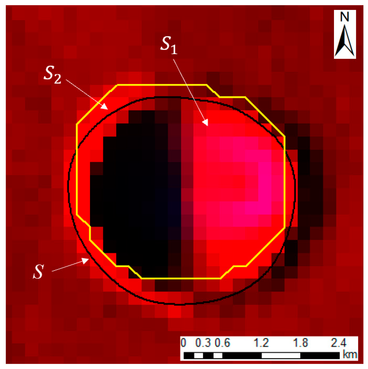
The above CDAs have made impressive strides. However, on the one hand, the existing CDAs based on deep learning only consider the morphological features of impact craters, often ignoring the geographic information involved. On the other hand, in quantity-oriented detection, the boundaries of impact craters are usually assumed to be circles. First, indeed, most researchers have focused on the quantity and radii/diameters of impact craters rather than their accurate boundaries. However, the morphological parameters, such as accurate diameters, accurate volumes, and boundary crushability, depend on accurate boundaries [39]. Accurate boundaries record the resurfacing caused by impacts, volcanic activity, hydrological effects, wind, and glacial erosion. Thus, accurate boundaries are important for the quantitative calculation of topographic parameters and for reflecting the degree of erosion. Furthermore, accurate boundaries can be used to deduce the history of surface degradation [26,27]. Second, obtaining accurate boundaries is essential for planetary geological and geomorphological mapping [40,41]. Notably, the identification of impact craters is time- and energy-intensive when mapping the global Moon. Third, accurate boundaries can be used to deduce the impact angle, impact direction, and impact crater formation mechanisms on slopes [42,43]. Fourth, the diameters of some impact craters are modified by linear tectonics. By calculating these diameters from accurate boundaries, the causal mechanisms of linear tectonics can be determined [44,45].

This study aimed to identify the accurate boundaries of impact craters, which is fundamental work. An impact crater dataset with large geographic coverage is useful for calculating morphological and topographic parameters, creating geological maps, and deducing the history of surface degradation and the causal mechanisms of linear tectonics. Therefore, it is crucial to study an automated algorithm for accurately identifying the boundaries of impact craters. To reduce the gap between circles and accurate boundaries, this article proposes a framework that combines geographic information and deep learning.

The main contributions of our work may be described as follows:

• For the first time, a benchmark dataset with annotations for identifying accurate boundaries of impact craters has been completed and made publicly available, and the sampling method considered the geographical distribution.
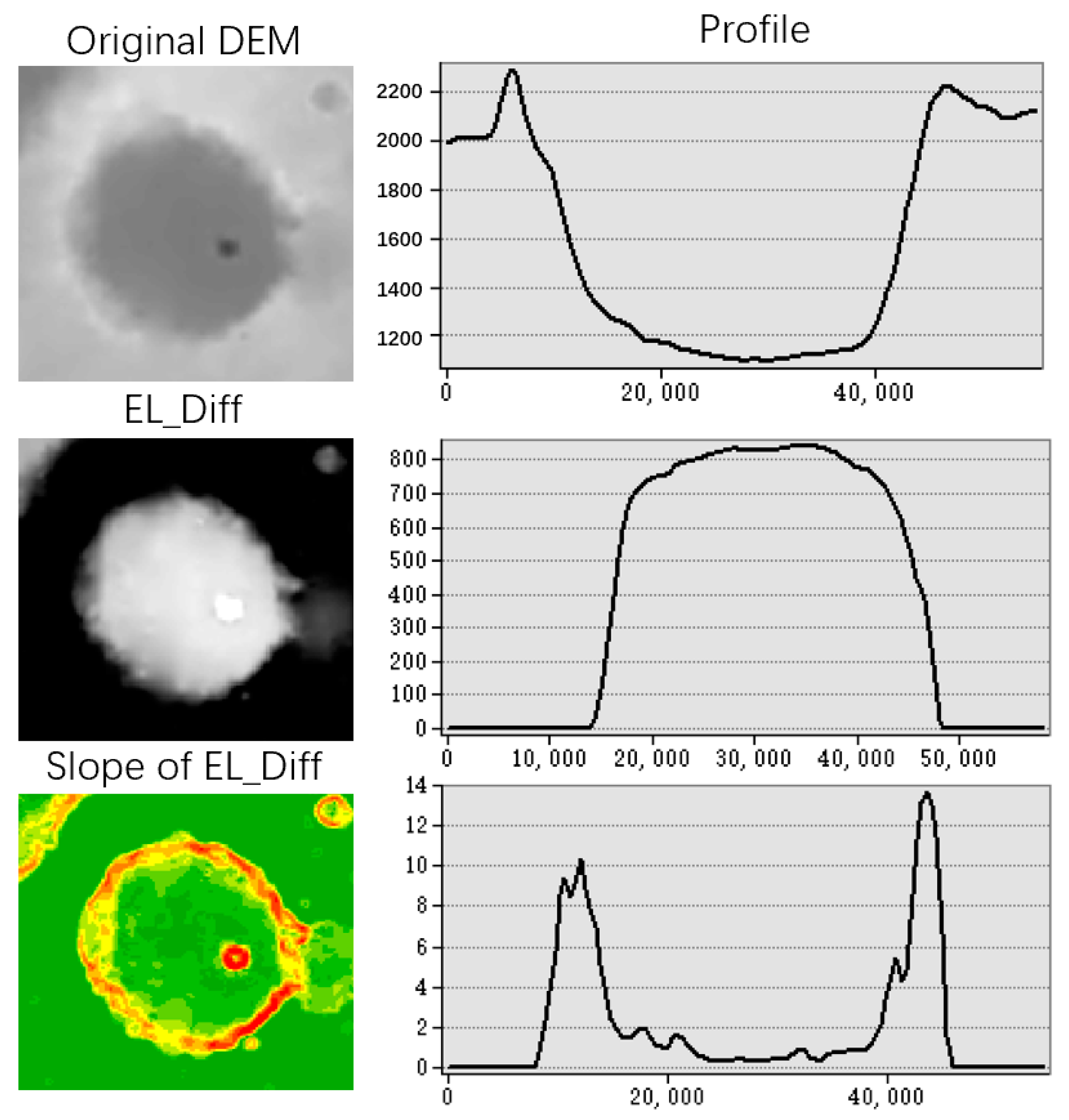
• Geographic information called the “slope of EL_Diff” was integrated into fusion data as model input. “Slope of EL_Diff” refers to the slope of elevation difference after filling the DEM in order to highlight the boundaries of impact craters.
• A framework called BDMCI was developed to accurately detect the boundaries of impact craters with a large geographic extent.

In this article, a system combining geographic information and deep learning is proposed to accurately detect the boundaries of Martian impact craters. The remaining sections of this article are as follows: The benchmark dataset with annotations and sample regions for the BDMCI framework is introduced in Section 2. The proposed BDMCI framework is presented in Section 3, which includes the model input, the introduction of two deep learning models, and postprocessing. In the experiment described in Section 4, the system was tested using fusion data from the Mars Orbiter Laser Altimeter (MOLA) and the Thermal Emission Imaging System (THEMIS), and a comparison was performed.

2. Study Area and Materials

2.1. Dataset Preparation

Fusion data are often used to detect impact craters [30,36] rather than relying on a single data source. As shown in Figure 1, the proposed BDMCI framework used fusion data integrated from optical images, DEM data, and slopes of EL_Diff. The optical images are Mars global mosaic images [46] obtained from THEMIS Day IR. The Thermal Emission Imaging System (THEMIS) is an instrument on board the Mars Odyssey spacecraft. The spatial resolution is 100 m per pixel. The geographic coverage of each optical image is 65°S–65°N, 0°E–360°E.

The blended DEM data [47] are derived from the Mars Orbiter Laser Altimeter (MOLA), an instrument onboard NASA’s Mars Global Surveyor (MGS), and the High-Resolution Stereo Camera (HRSC), an instrument onboard the European Space Agency’s Mars Express (MEX) spacecraft [48,49]. The spatial resolution is 200 m per pixel. The geographic coverage of the DEM is global. To reduce the projection distortion along the parallels towards higher latitudes, we clipped the DEM to the same geographic area (65°S–65°N, 0°E–360°E). The map projection of the optical image and DEM is a cylindrical equidistant (simple cylindrical) map projection, with the Mars spheroid as defined by IAU 2000 as a reference. The semimajor axis and semiminor axis are both 3396.19 km, and inverse flattening is 0. Although there are some other datasets (e.g., Mars Reconnaissance Orbiter Context Camera) with higher spatial resolution, the purpose of this article is to detect accurate boundaries of Martian impact craters with a large geographic extent. The amount of computation increases with increasing spatial resolution. The mosaic work was too expensive in terms of time and computation. Furthermore, it is enough to identify the impact craters over a large geographic area. The spatial resolution of DEM is almost 200 m/px, which is higher than the 232 m mosaics from Viking MDIM2.1 and the 463 m mosaics from MGS MOLA. Thus, we chose a 100 m optical image and a 200 m DEM to train and test the proposed BDMCI framework. As shown in Figure 1, to better fit the structure and parameters of the deep learning models, the three datasets (DEM, optical image, and slope of EL_Diff) were normalized into the same range [36] before inputting the data into the deep learning models.

2.2. Processing the DEM with Geographic Information

The slope of EL_Diff is the slope of the elevation difference between the filled DEM and the original DEM. Impact craters can be thought of as depressions caused by impacts. Virtually, if rain falls from the sky, the impact crater will be filled by the rain. The differences in elevation could indicate the boundaries of impact craters. This geographic information was introduced in the preprocessing stage before inputting the data into the deep learning models.

Figure 2 shows the two methods of data processing. In the first method, the slope of slope was calculated from the original DEM using the slope twice. In the second method, the slope of EL_Diff was calculated. First, the impact craters were filled. Second, the filled DEM was subtracted from the original DEM. Third, the slope of the results of the second step was calculated. The slope of EL_Diff highlighted the boundaries of impact craters (red parts in Figure 2) and reduced the stripe noise in the DEM data compared with that using the slope of slope, as shown in Figure 2. In Figure 3, the boundary of the crater was highlighted by “Slope of EL_Diff” in the profile view and compared with the original DEM. Additionally, the spatial resolution, geographic coverage, and map projection of the slope of EL_Diff are the same as those of the DEM, as shown in

Table 2. Details of DEM, optical image, and slope of EL_Diff.

Data Source	Spatial Resolution	Extent	Map Projection
Blended DEM from MOLA and HRSC	200 m/px	Global	Plate_Carree
THEMIS Day IR	100 m/px	65°S–65°N, 0°E–360°E	Plate_Carree
Slope of EL_Diff	200 m/px	Global	Plate_Carree
Fusion data	200 m/px	65°S–65°N, 0°E–360°E	Plate_Carree

.

2.3. Sample Area Selection

The Martian surface is more complicated than the lunar surface. The former contains glacial, volcanic, aeolian, and fluvial landforms, which could influence the detection of impact craters. In this article, six sample areas were selected to prepare a benchmark dataset with annotations and test the proposed BDMCI. These six regions included the boundary between the northern and southern hemispheres, the northern plain, the edge of the Hellas Basin, the Marineris Valleys, and ordinary areas. Each sample size was 1024 × 1024 pixels. After gridding the sample area into squares, geospatially stratified and optimized sampling [50,51,52] was used to select sample areas, as shown in the “Sample area selection” in Figure 4. This sampling method yielded representative training samples and reduced the workload of the preparation of the benchmark dataset with annotations.

First, the central points were calculated from the sample grids. A total of 1352 grids with central points and six regions were prepared for selection. Second, the average distance between central points was maximized using simulated annealing. Half of the central points were set to be preserved. The goal of geospatially stratified and optimized sampling was for sample points to be widely distributed throughout the study area. Finally, the sample area according to the sample points was selected as the input for the subsequent step.

2.4. Benchmark Dataset with Annotations

The performance of a model is directly affected by the quality of the applied benchmark dataset with annotations. Recent studies focused on detecting impact craters rarely propose benchmark datasets with annotations, especially those with accurate boundaries for impact craters. Geo AI Martian Challenge (http://cici.lab.asu.edu/martian/#home (accessed on 13 October 2022), [31]) is a popular open dataset that originated from a collaboration between Arizona State University, the United States Geological Survey, the Jet Propulsion Laboratory, Oak Ridge National Lab, Esri, Google, and the American Geographical Society. This challenge provides an impact crater dataset with annotations marked by bounding boxes, and the detection of accurate boundaries of impact craters is difficult.

A benchmark dataset with annotations of accurate boundaries of Impact craters was developed, as shown in Figure 5, and made available to the general public. With the fusion data displayed as a base map, accurate boundaries of impact craters were marked by polygons according to a comprehensive assessment. In this benchmark dataset with annotations, the impact craters with diameters larger than 2 km were preserved.

3. Methods

According to Liu et al. [26] and Chen et al. [27], impact craters include dispersal craters, connective craters, and con-craters (con-craters refer to nested craters containing dispersal craters and connective craters). To detect the above impact craters, the idea of object orientation should be introduced. The outputs of object detection are the boundary box and category, and the output of semantic segmentation is the category of each pixel. Object detection and semantic segmentation may ignore the boundaries of connective craters and con-craters. The outputs of instance segmentation are pixel-level classification results, and this approach is more suitable for detecting impact craters. In this study, Mask2former, Mask R-CNN, SOLOv2, Cascade Mask R-CNN, and SCNet were selected to be trained on detecting impact craters.

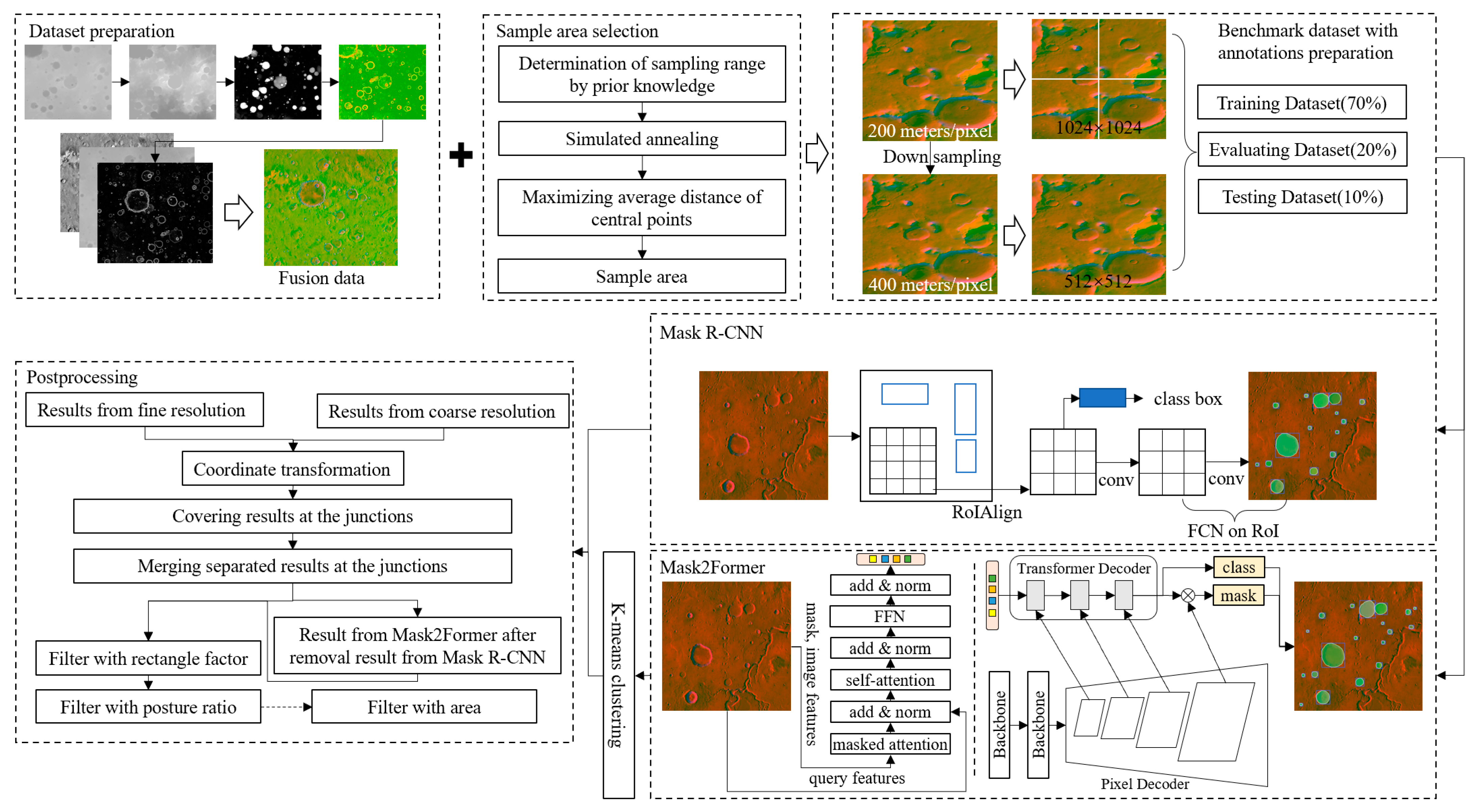
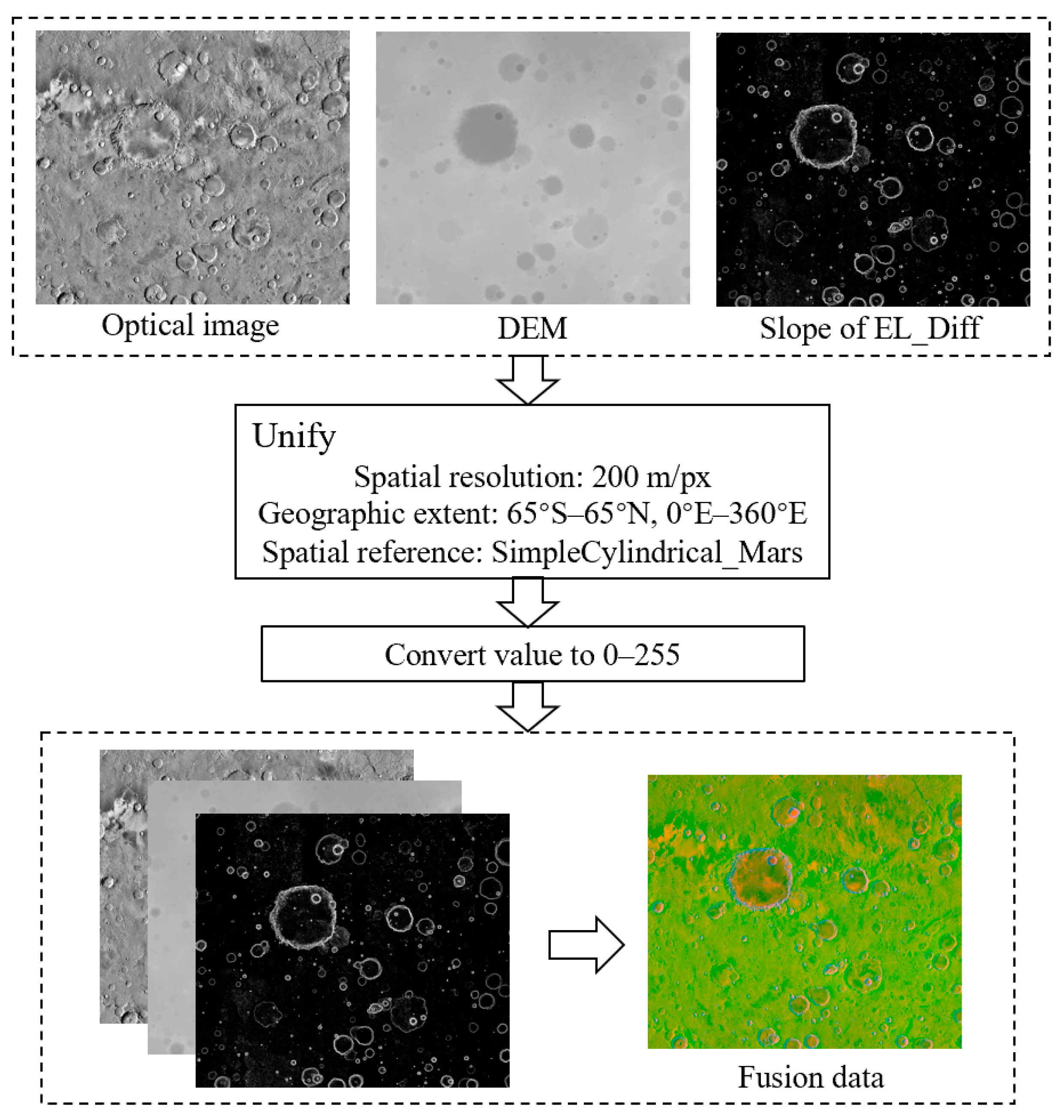
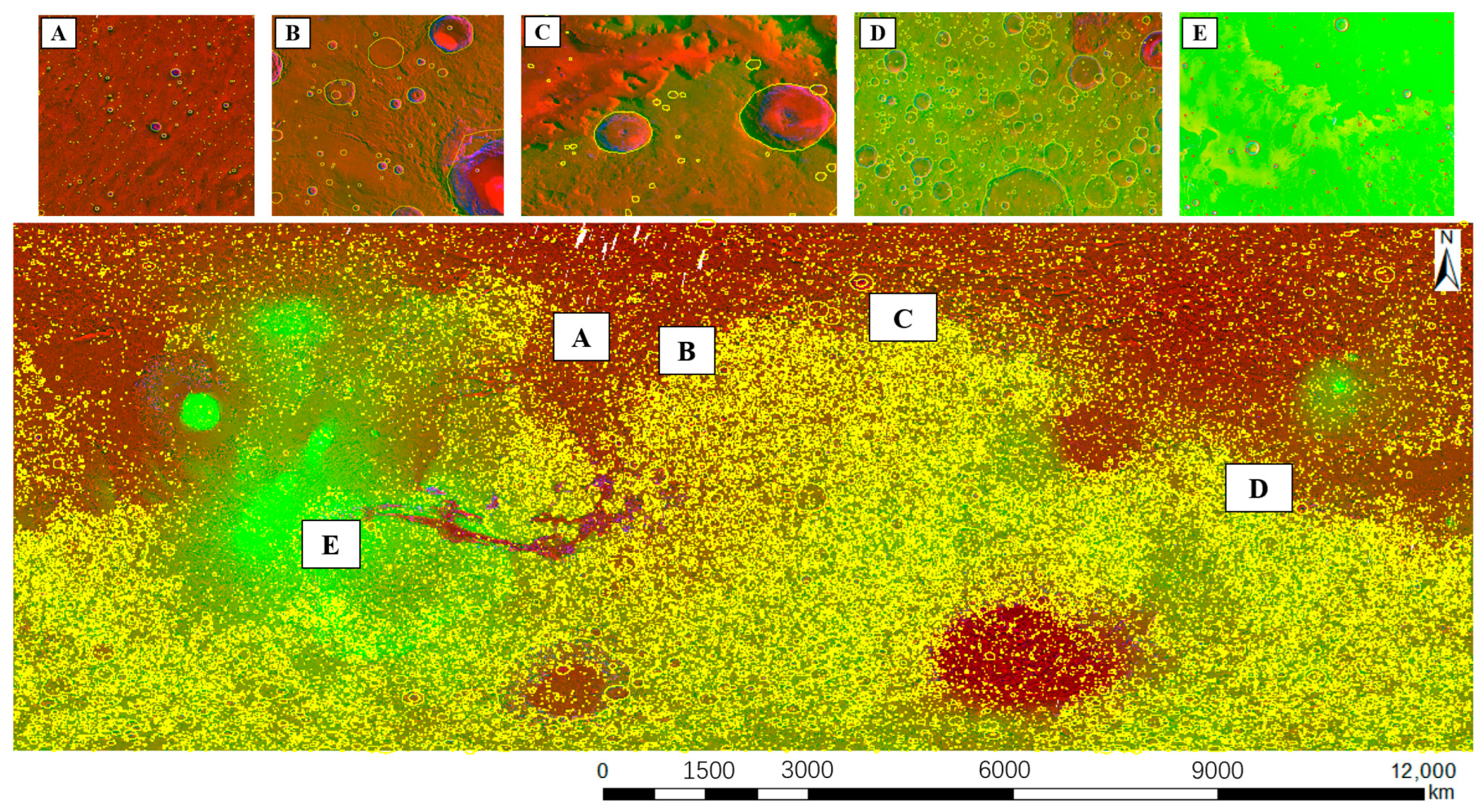
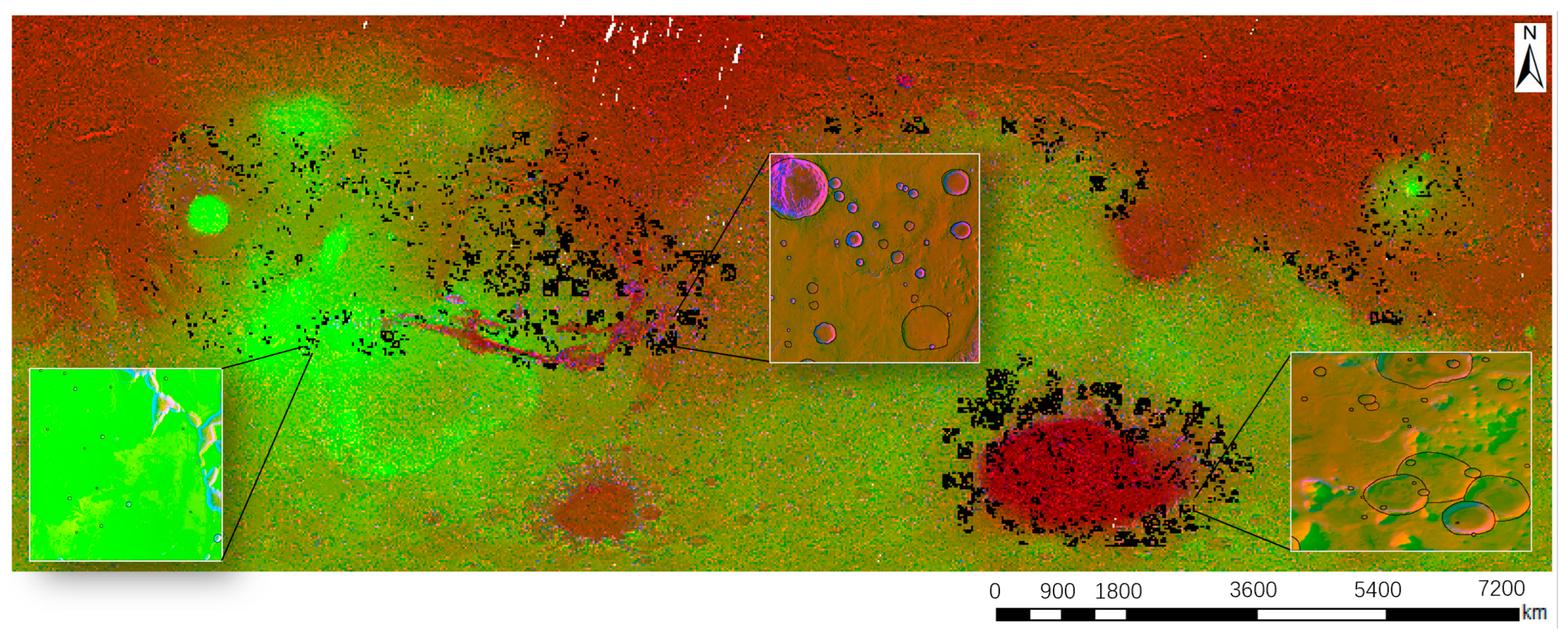
An overview of the proposed BDMCI framework is shown in Figure 6. In the dataset preparation stage, the DEM, optical image, and slope of EL_Diff (as stated in Section 2.2) were integrated into the fusion data. The fusion data contain elevation, grayscale information, and the highlighted boundaries of terrain. In the sample area selection stage (Section 2.3), the sampling range was determined based on prior knowledge. The sample area was selected using simulated annealing and maximizing the average distance from central points. After data preparation and sample area selection, the benchmark dataset with multiscale images and annotations was input into Mask R-CNN and Mask2Former. The results from Mask2Former were processed by K-means clustering and then merged with the results from Mask R-CNN. Finally, the merged results were postprocessed to identify the fractures at junctions and filter out the false results. This framework can be used to identify accurate boundaries of Martian impact craters with geographic information and deep learning. The impact craters between 65°S–65°N, 0°E–360°E were identified using this framework, as discussed in Section 4.6.

3.1. Model Input

The input data of the model are the fusion data mentioned in Section 2.1. The first channel is the optical image. The second and third channels are the DEM and the slope of EL_Diff, respectively. The proportion of training to validation to testing is 7:2:1, which ensures that the number of training sets needed to enhance the model is sufficient. There were 451 patches in the six sample areas. The size of the patches was 1024 pixels, with a spatial resolution of 200 m/px. These patches were randomly proportionally divided into a training set, a validation set, and a test set. The training set had 316 patches, the validation set had 90 patches, and the test set had 45 patches. In addition, these three sets did not overlap. The fusion data and benchmark dataset with annotations were clipped based on the divided grids. Images and annotations were input into the models in the format of the Microsoft Common Objects in Context (MS COCO) dataset. Finally, the geographical coordinates were converted into image coordinates.

Impact craters vary in size, which makes identification quite difficult. The diameter of a small impact crater might be 200 m, while the diameter of a large impact crater might be 200 km. Thus, a multiscale dataset was input into the model. Additionally, upsampling might generate some potential artifacts, so the spatial resolution of the fusion data was changed from 200 m/px to 400 m/px through downsampling. Images with pixel sizes of 512 × 512 and 1024 × 1024 were created in MS COCO before being input into the model to potentially improve the identification of multiscale impact craters.

3.2. Fusing Multiple Models

3.2.1. Mask2Former

The masked-attention mask transformer (Mask2Former) [53] uses mask classification for segmentation and detection. Masked attention, which is used to extract local features by restricting cross-attention to the anticipated mask area, is a crucial part of Mask2Former. To help the model segment small items or regions, Mask2Former uses multiscale, high-resolution features, as shown in Figure 5. Local features were extracted by limiting cross-attention to the foreground area of the prediction mask in each query rather than focusing on the complete feature map. Compared to the traditional CNNs, the transformer introduces a self-attention mechanism to focus on local information and identify more small impact craters. Thus, Mask2Former was considered the basic model.

However, transformers lack some of the inductive biases inherent to CNNs, such as translation equivariance and locality, and therefore do not generalize well when trained on insufficient amounts of data [54,55]. Thus, Mask2Former requires a large benchmark dataset with annotations. In the case of an insufficient benchmark dataset, the boundaries of impact craters would be disturbed by local information. Nevertheless, if a large benchmark dataset with annotations of Martian impact craters were produced, the advantage of automated identification would disappear. To balance the performance and efficiency of identification, it is necessary to combine another model to solve the problem of false positive boundaries.

3.2.2. Mask R-CNN

Mask R-CNN [56] can not only output bounding boxes but also masks with labels. It extends Faster R-CNN [57] by adding a small fully convolutional network (FCN) in parallel with the existing branch. Faster R-CNN is designed for classification and bounding box regression. The FCN is designed to predict segmentation masks. With the accurate pixel mask of the FCN, the result is highly accurate. In addition, the use of RoIAlign instead of RoIPooling solves the misalignment problem caused by direct sampling through pooling, which has a large error in the pixel-level mask. RoIAlign makes the pixels in the original image and the pixels in the feature map perfectly aligned, which not only improves the detection accuracy but also facilitates instance segmentation.

Mask R-CNN requires two stages to perform classification, namely, regression and segmentation, as shown in Figure 5. The first stage is at the same level as the RPN in Faster R-CNN, and it involves scanning images and generating area proposals. In the second stage, a branch of a fully convolutional network is added, as well as category prediction and bounding box regression. Every region of interest (RoI) could be predicted by the corresponding binary mask to mark whether the pixel is part of an object.

3.2.3. Model Selection

This method is a strategy of fusing multiple models, which is a simple method in the ensemble learning field. On the one hand, the transformer has a self-attention mechanism that can better focus on local information, while Mask R-CNN has better scale invariance features. Integrating the models of these two modes can leverage their common advantages. On the other hand, while the benchmark dataset was already sufficient for Mask R-CNN, the transformer requires a large amount of data for training. To prevent inadequate training of the transformer, Mask R-CNN can be used to supplement it. The ability of Mask R-CNN to identify all crater instances is insufficient and can be made up through a transformer.

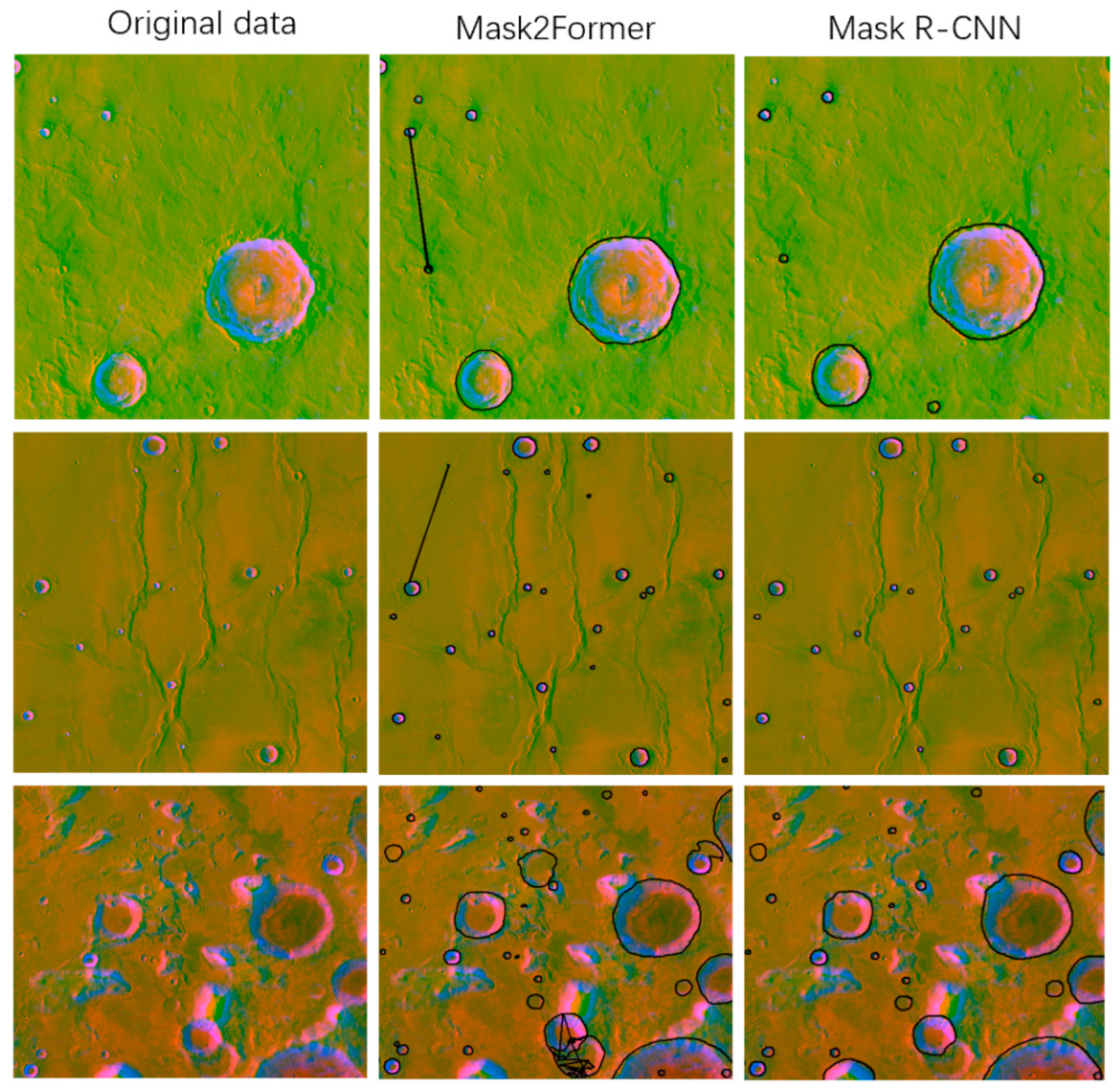
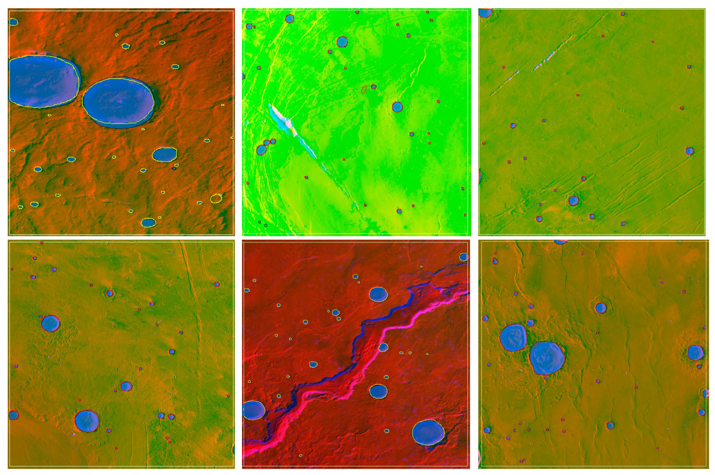
Figure 7 depicts the detection results obtained with Mask2Former and Mask R-CNN. In the second column of Figure 7, while detecting more small craters than Mask R-CNN, Mask2Former also brings many negative effects (the results that were associated with the same crater) due to an insufficient benchmark dataset. In the third column of Figure 7, while Mask-RCNN missed some small craters, it could avoid the excessive influence of tiny terrain compared with Mask2Former. After the experiments in Section 4, we found that the method “Mask R-CNN + Mask2former” performed the best. Finally, “Mask R-CNN + Mask2former” was constructed to identify impact craters with a large geographic extent.

3.3. Postprocessing

The results detected by Mask R-CNN and Mask2Former were both image coordinates. The coordinates were within the range of (0~511). To build Martian impact crater catalogs, it was necessary to transform the image coordinates into geographical coordinates.

In this study, the inputs of the deep learning model were scaled to 512 × 512 pixels in Mask R-CNN, as noted in Section 3.1. Fractures existed at the junctions of patches. Because the input images were nonoverlapping, the craters at the junctions could not be detected. Multiscale results were integrated to solve this problem.

3.3.1. Coordinate Transformation

This process is called affine transformation. Six parameters were needed for the affine transformation: the geographical coordinates of the upper left corner of the image, the horizontal and vertical spatial resolution of the image, and the image rotation coefficient. Image coordinates ($col$, $row$) were transformed into geographic coordinates ($x_{geo}$, $y_{geo}$) with Equations (1) and (2).

$$x_{geo}=\mathrm{t}\mathrm{r}\mathrm{a}\mathrm{n}\mathrm{s}\left[0\right]+col\times \mathrm{t}\mathrm{r}\mathrm{a}\mathrm{n}\mathrm{s}\left[1\right]+row\times \mathrm{t}\mathrm{r}\mathrm{a}\mathrm{n}\mathrm{s}\left[2\right]$$

(1)

$$y_{geo}=\mathrm{t}\mathrm{r}\mathrm{a}\mathrm{n}\mathrm{s}\left[3\right]+col\times \mathrm{t}\mathrm{r}\mathrm{a}\mathrm{n}\mathrm{s}\left[4\right]+row\times \mathrm{t}\mathrm{r}\mathrm{a}\mathrm{n}\mathrm{s}\left[5\right]$$

(2)

where trans[0] and trans[3] are the x and y coordinates of the upper left corner of the image, respectively; trans[1] and trans[5] are the horizontal and vertical spatial resolution of the image, respectively; and trans[2] and trans[4] are the image rotation coefficients. For the north-up images, trans[2] and trans[4] are equal to zero, and col and row are the row and column numbers of pixels in the image, respectively.

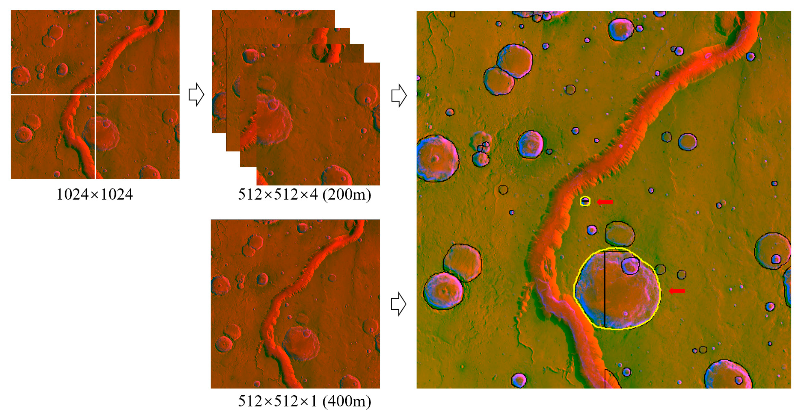
3.3.2. Covering the Results at Junctions

The above models could detect the craters at the junctions of images. However, obvious fractures were shown in the results. A total of 1024 × 1024 pixel patches with a spatial resolution of 200 m/px were clipped directly from the fusion data and then clipped again into 512 × 512 pixels, called fine-scale data. The 512 × 512 pixel patches with a spatial resolution of 400 m were clipped directly from fusion data, called coarse-scale data. The domains of the two datasets were different, while the number of grids was the same, as shown in Figure 8. The domain of coarse-scale data was four times larger than the domain of fine-scale data. Fine-scale and coarse-scale patches were input into the models. The results based on fine-scale and coarse-scale data were obtained after running the above models. In the test regions, the split lines (white lines in Figure 8) were calculated. Then, the results from the fine-scale data and the split lines were intersected to obtain the yellow lines in Figure 8. The fine-scale results at the junctions are covered by yellow lines (from the coarse-scale data).

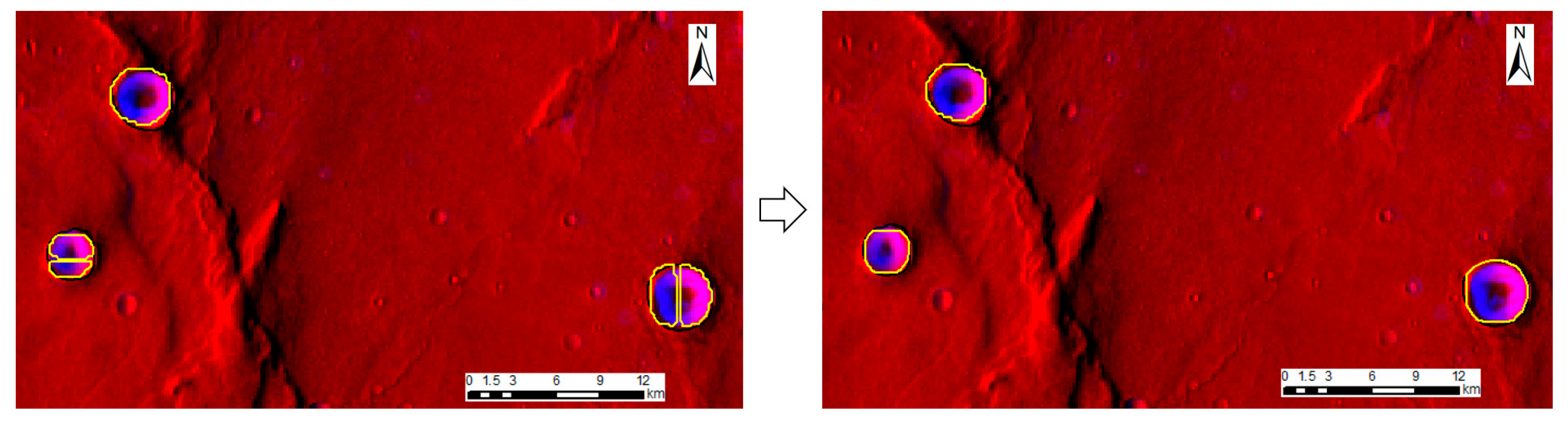
3.3.3. Merging Separate Results at the Patch Junctions

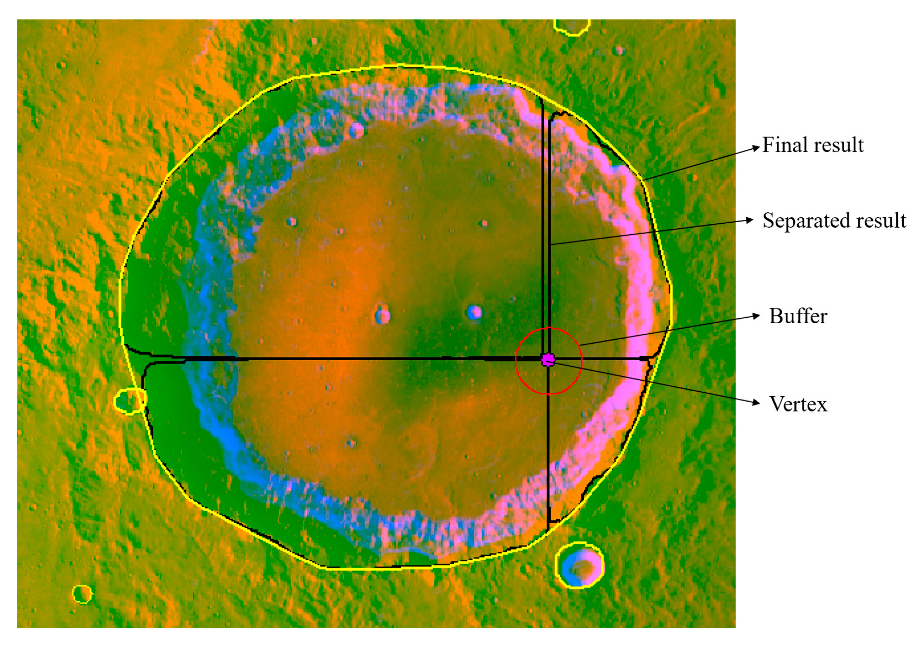
After covering the separate results at the junctions by calculating split lines, several separate results remained. For the results near the vertices of the patches, the associated identifiers were modified by obtaining the buffers of vertices, as shown in Figure 9. Thus, the identifiers of the same impact crater were set to the same number. For the results on the edges of patches, the associated identifiers were modified manually, as shown in Figure 10. Then, the corresponding convex hull was calculated to merge the separate results into a complete crater.

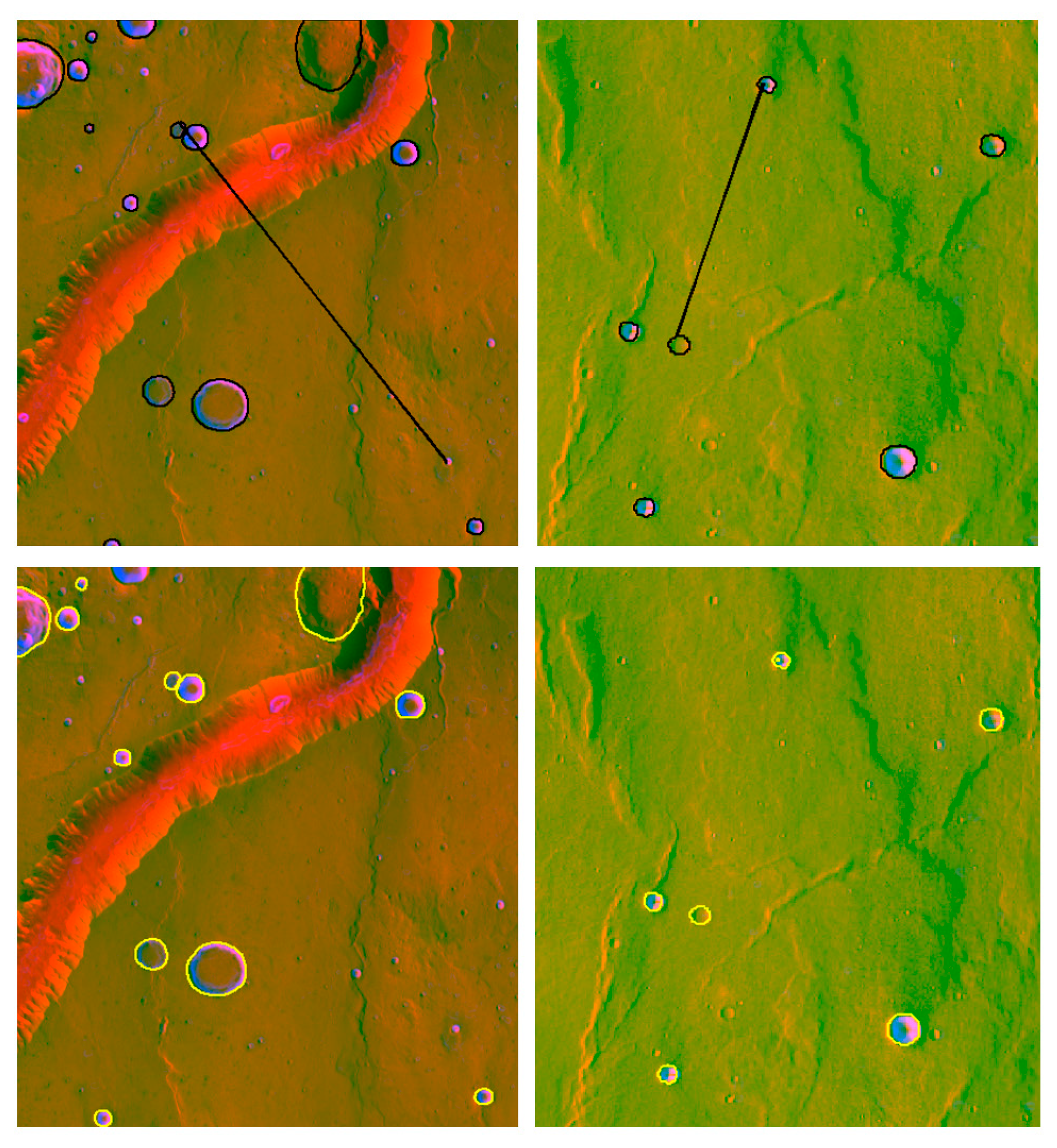
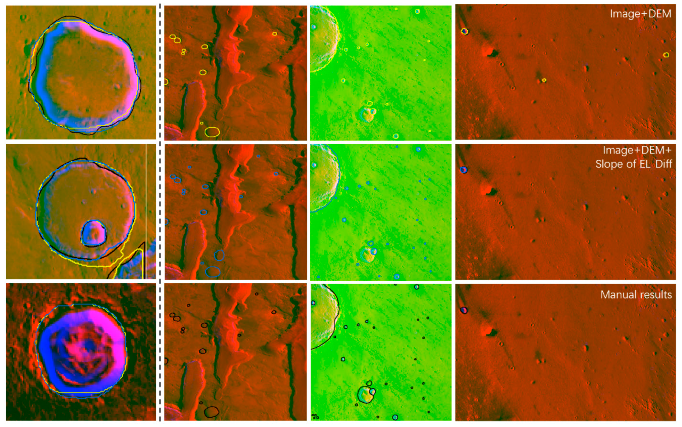
3.3.4. K-Means Clustering for the Detection Results of Mask2Former

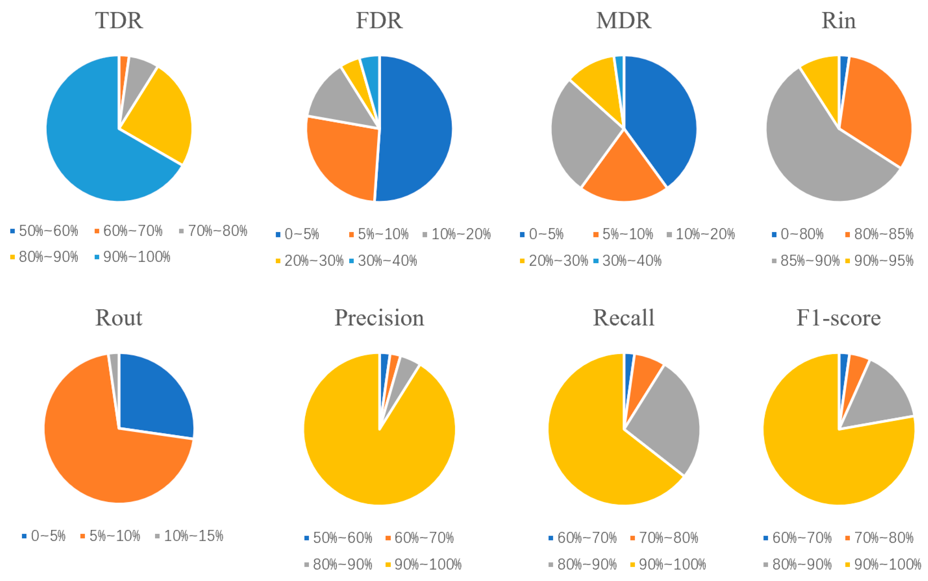
As shown in Figure 11, two or three craters detected by Mask2Former might be connected, and the points belonging to different impact craters were mixed. To separate the mixed points, k-means clustering [58] was used for classification. It is very important to determine the k value, which is the number of clusters. Based on the elbow method, with the increased cluster number k, the sample division becomes increasingly refined. Thus, the degree of aggregation of each cluster gradually increases, and therefore, the sum of the squared errors (SSE) naturally decreases. The k value was set to 0.6 after comparing the performance of several k values.

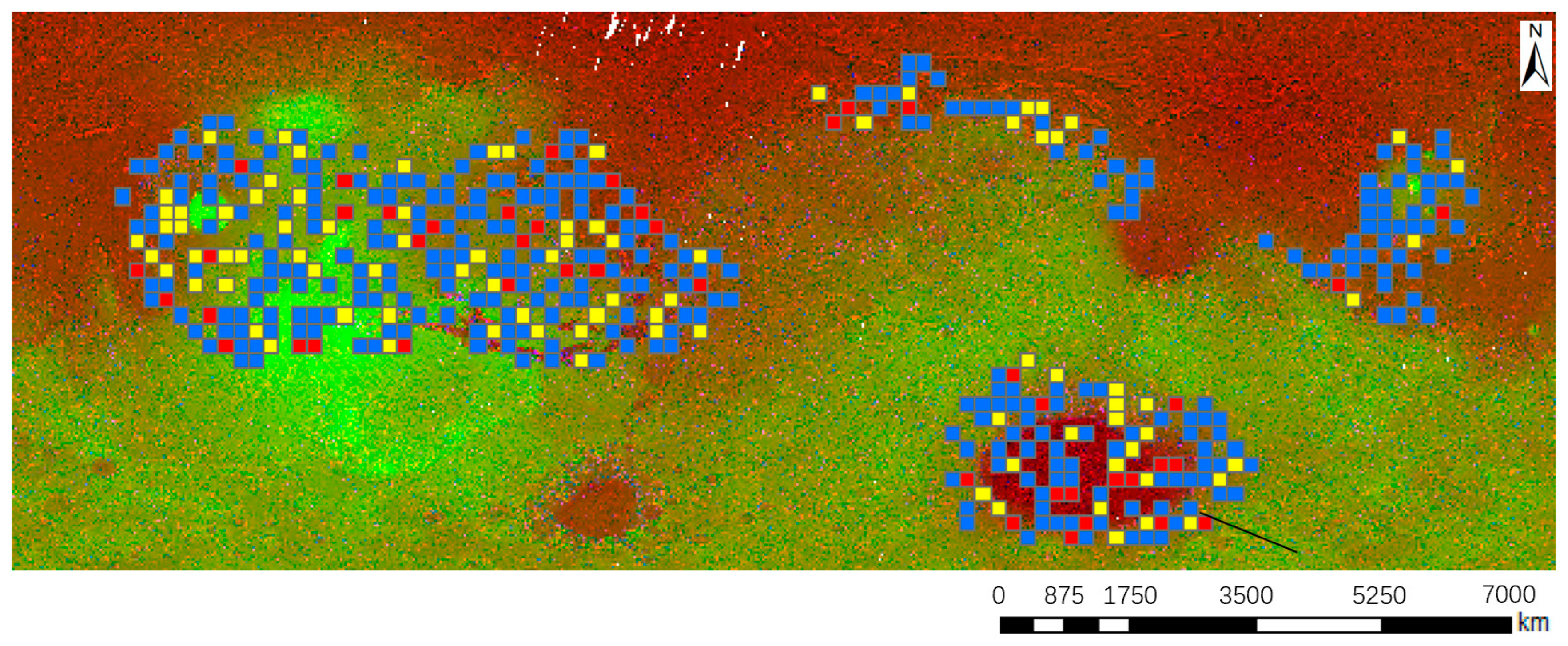
3.3.5. Filter with Morphological Parameters

To filter the false results from Mask R-CNN and Mask2Former, morphological parameters, such as the posture ratio, rectangle factor, and area, were used for postprocessing. Their definitions are given as follows:

(A)

Posture ratio

The posture ratio refers to the ratio between the long side and the short side of the minimum bounding rectangle (MBR). The posture ratio was used to filter the results that were associated with the same crater (the negative effects in the second column of Figure 7). In general, the MBR of these results was a rectangle with a high posture ratio. The posture ratio was calculated as follows using Equation (3):

$$c_1=\frac{L}{W}$$

(3)

where L is the length of the MBR, W is the width of the MBR, and $c_1$ is the posture ratio of the impact crater.

(B)

Rectangle factor

The rectangle factor refers to the ratio between the area of the impact crater and the area of the corresponding MBR. The rectangle factor reflects the fullness in the MBR, which can be calculated using Equation (4):

$$c_2=\frac{A_o}{A_r}$$

(4)

where $A_o$ is the area of the impact crater, $A_r$ is the area of the MBR, and $c_2$ is the rectangle factor of the impact crater.

After filtering with the posture ratio and rectangle factor, the results from Mask2Former were filtered based on the area because many small craters with diameters smaller than 2 km were identified.

4. Experiment and Results

4.1. Modeling Configuration

In this article, Mask R-CNN and Mask2Former were both constructed in Anaconda3/5.3.0 and PyTorch v11.2. The models were run on Linux and Tesla v100. The initial learning rate and momentum were set to 0.001 and 0.9, respectively. In addition, the weight decay coefficient was set to 0.0001. The optimization method of the models was stochastic gradient descent (SGD) with 150 epochs. For Mask R-CNN, ResNet-50 [59] was used as the basic network to train the model. The pretrained parameters were used to initialize the model on a feature pyramid network (FPN) [60]. For Mask2Former, ResNet-50 was also used as the basic network. The pretrained parameters were used to initialize the model on ImageNet [61]. Then, all the parameters of the network were fine-tuned using the benchmark dataset with annotations and corresponding fusion data. Impact craters with diameters greater than 2 km were included in the benchmark dataset with annotations.

4.2. Threshold of Morphological Parameters

Impact craters have shapes similar to circles. As a result, their minimum bounding rectangles were squares. The relationship between impact craters and MBR was discussed according to Liu et al. [26]. The threshold of the rectangle factor for dispersal impact craters was 0.69. The shapes of impact craters in high-latitude regions are often similar to rectangles due to projection distortion with large geographic coverage. The threshold of the posture ratio was 2. The size of the impact craters that could be distinguished was approximately 5 × 5. At a spatial resolution of 200 m/px, the threshold of the area for filtering results that were too small was 1,000,000 m². Finally, the results from Mask2Former after filtering with morphological parameters and the results of Mask R-CNN were merged to produce the final results.

4.3. Evaluation of the Proposed BDMCI Framework

The manual results used to evaluate the performance of this method were from the benchmark dataset with annotations, as shown in Figure 5. The manual results were identified from the optical image, hillshade, slope of EL_Diff, and slope. The test areas are shown in Figure 12 (red grids). The spatial resolution of the fusion data was 200 m/px. The size of a patch was 1024 × 1024 pixels, which was clipped to four patches of 512 × 512 pixels. Due to the 200 m spatial resolution, the maximum diameter of the detected impact craters was 204.8 km.

Accurate boundaries of impact craters focus not only on their position but also on the precision of those boundaries. Therefore, the factors used to evaluate the proposed BDMCI framework reflected quantity, namely, the true detection ratio (TDR), the missed detection ratio (MDR), and the false detection ratio (FDR), as well as quality, particularly $R_{in}$ and $R_{out}$. TDR, MDR, and FDR were proposed by Zhang et al. [62]. $R_{in}$ and $R_{out}$ were proposed by Liu et al. [63]. However, several small and obscure impact craters were missing when impact craters with a large geographic extent were manually identified. These impact craters were detected by the proposed BDMCI framework, and they were used to supplement the manual identification results. Thus, some improvements were made based on TDR, MDR, FDR, $R_{in}$, and $R_{out}$, as shown in Equations (5)–(11).

$$\mathrm{S}\mathrm{U}\mathrm{M}=\mathrm{M}\mathrm{I}+\mathrm{S}\mathrm{M}\mathrm{I}$$

(5)

$$TP=\mathrm{T}\mathrm{D}+\mathrm{S}\mathrm{M}\mathrm{I}$$

(6)

$$\mathrm{M}\mathrm{D}\mathrm{R}=\frac{MD}{SUM}$$

(7)

$$\mathrm{T}\mathrm{D}\mathrm{R}=\frac{TP}{SUM}$$

(8)

$$\mathrm{F}\mathrm{D}\mathrm{R}=\frac{FD}{TP+FD}$$

(9)

where MI is the result of manual identification, SMI is the supplement to the manual identification results, SUM is the sum of manual identification and the missed detections from manual identification, and TD, MD, and FD are the numbers of true detection, missed detection, and false detection, respectively.

$$R_{in}=\frac{S_1}{S}$$

(10)

$$R_{out}=\frac{S_2}{S}$$

(11)

where $R_{in}$ and $R_{out}$ are the ratios of automatically detected results that fall within and outside of the set of manually detected results, respectively. The diagram of $R_{in}$ and $R_{out}$ is shown in Figure 13. By intersecting the automatically detected results and the manual results, S₁ is the area of the portion of the automatically detected results in the manual results, and S₂ is the area of the portion of the automatically detected results outside the manual results. S is the area of the manual results.

In addition, precision, recall, F1-score, and Intersection over Union (IOU), as shown in Equations (12)–(15), were also used to evaluate the proposed method.

$$Precision=\frac{TP}{TP+FD}$$

(12)

$$Recall=\frac{TP}{TP+MD}$$

(13)

$$F1\text{-}score=\frac{2\times Precision\times Recall}{Precision+Recall}$$

(14)

$$IOU=\frac{Intersection}{Union}$$

(15)

where Intersection and Union are the intersection and union of the automated and manual results, respectively.

The criteria for evaluation were as follows:

• The craters at the border were often clipped and incomplete. Their area was the basis for determining whether to count them. If the area of the impact crater was only half or less reserved, this crater was ignored in the true detection results as well as in the manual identification results.
• If the results detected by the proposed BDMCI framework and the manual results coincided, they were considered true detection results.
• If the results detected by the proposed BDMCI framework and the manual results did not coincide, it was necessary to review the fusion data. If the results based on the fusion data indicated the presence of impact craters and their diameters were larger than 2 km, they were used as a supplement for manual identification (SMI); otherwise, they were false detections.
• If the diameters of the results were smaller than 2 km, the results were individually labeled and not counted in the statistics.

The evaluation of the proposed BDMCI framework in the test region based on the above criteria is shown in

Table 3. Evaluation of the proposed BDMCI framework in the test regions. (See Appendix A Table A1 and Table A2 for details.)

TDR	92.35%	Precision	94.25%
FDR	8.60%	Recall	91.76%
MDR	8.31%	F1-score	92.99%
Rin	86.02%	IOU	90.21%
Rout	5.61%

and Figure 14. These 45 test regions were selected randomly and included plains, highlands, basins, volcanoes, valleys, and the junctions between the northern and southern hemispheres. Notably, these landforms are easily confused with impact craters. Craters were then detected even in these regions. Based on the evaluation of accuracy in these regions, the proposed BDMCI framework displayed strong universality and robustness.

The TDR in most test regions was greater than 90%, as shown in Figure 15. Both the FDR and MDR in most of the test regions were less than 9%. These pie charts were created based on the frequency of test regions distributed in different precision intervals.

4.4. Comparison with MA132843GT

For D ≥ 2 km, MA132843GT is a relatively complete published catalog of crater information [10]. This catalog was published by G. Salamunićcar and his team. Thus, MA132843GT was considered another benchmark for validation. It was finished by combining manually detected results with automatically detected results after constant updates using THEMIS DIR and MOLA. The results in the 45 test regions were also compared with MA132843GT, as shown in

Table 4. Comparison of the results and MA132843GT in the test regions. (See Appendix A Table A3 for details.)

TDR	96.65%	Precision	95.08%
FDR	4.92%	Recall	96.61%
MDR	3.40%	F1-score	95.49%

. The TDR, FDR, and MDR were 96.65%, 4.92%, and 3.40%, respectively. The precision, recall, and F1-score were 95.08%, 96.61%, and 95.49%, respectively.

4.5. Comparison with Other Models and Ablation Experiments

Different models and their combinations were used for comparison with the proposed framework. From

Table 5. Comparison of the proposed model and other models.

Models/Data	Precision	Recall	F1-Score	IOU
Mask R-CNN	96.28%	68.33%	78.80%	90.45%
Mask2Former	92.69%	91.31%	91.44%	89.19%
SOLOv2	93.81%	64.43%	74.86%	86.99%
Cascade Mask R-CNN	96.24%	70.33%	80.11%	90.48%
SCNet	97.54%	67.87%	79.09%	90.82%
Cascade Mask R-CNN + Mask2Former	94.28%	91.35%	92.15%	90.04%
SCNet + Mask2Former	93.12%	90.92%	91.61%	90.08%
Mask R-CNN + Mask2Former	94.25%	91.76%	92.99%	90.21%
Ablation experiments
Image + DEM	90.91%	84.66%	86.74%	89.87%

, Mask2Former has excellent performance compared to the other models. However, the results from Mask2Former include the connecting results in Figure 11 (black lines). Thus, it is necessary to combine other models to improve performance. Mask R-CNN was used by Tewari et al. [36] to detect lunar impact craters. In addition, the F1-scores of Cascade Mask R-CNN and SCNet achieved 80.11% and 79.09%, respectively. These three models were combined with Mask2Former, and the results are shown in Table 5. The performance of models combined with Mask2Former was remarkably better than that of other single models. Among these combined models, the recall and F1-score of Mask R-CNN and Mask2Former were the best.

Fusion data including the image, DEM, and slope of EL_Diff were used in the proposed method. To test the effect of the slope of EL_Diff, the image and DEM were used as the inputs of the proposed method in the ablation experiments. The precision, recall, F1-score, and IOU are shown in Table 5. On the left side of Figure 16, the results from the three types of data were closer to the manual results than the results from the image and DEM. In Figure 16, on the right side, some false results disappeared, and some true results appeared in the results from the three types of data compared to the results from the image and DEM.

4.6. Detection Results over a Large Geographic Area

Automated detection methods for impact craters are generally applied globally or over a large geographic area. In this article, we applied the proposed BDMCI framework to the region between 65°S and 65°N. The fusion data were integrated with the optical image, DEM, and slope of EL_Diff. The spatial resolution of the fusion data was 200 m/px. The large geographic area was clipped to 512 × 512-pixel patches. These nonoverlapping patches were input into the proposed BDMCI framework. The vertices of patches and their buffers were calculated. The buffer distance was set to 4000 m (200 m × 20 pixels). Then, the detected results were merged into a shapefile. Convex hulls were obtained to merge the separated results at the junctions. This step combined the results around the vertexes that belong to the same crater. The results after manual fine-tuning in the region between 65°S and 65°N are shown in Figure 17.

5. Conclusions

In this article, a deep-learning-based CDA called the BDMCI framework was proposed to detect Martian impact craters with a large geographic extent as well as accurate crater boundaries. A benchmark dataset with annotations for accurate boundaries available to the general public was obtained and input into the model, including the Mask R-CNN and Mask2Former submodels. Quantitative and qualitative comparisons were performed in the experiments. The evaluation showed that the proposed method was suitable for craters with diameters of 2~204.8 km. The detected results were compared with MA132843GT. Furthermore, the results in 45 test regions demonstrated that the proposed BDMCI framework provides a high generalization ability for different geomorphic types. Nevertheless, some limitations still need to be addressed:

• Although the impact craters at the junctions could be detected, the depressed terrains similar to impact craters were also detected as noise with the proposed CDA. The noise, which often leads to false positives, might be caused by fluvial and glacial erosion on Mars. This effect is especially strong at the edges of patches. Impact craters are randomly formed, and the distribution of the depressions formed by fluvial and glacial erosion is often regular. Thus, fluvial and glacial erosion data might be useful to remove noise.
• The proposed BDMCI framework based on a multiscale concept (200 m and 400 m, as stated in Section 3.3.2) could detect the impact craters at the junctions between patches, but this approach is slightly cumbersome for global detection. Moreover, Mask2former requires a large benchmark dataset with annotations to detect the impact craters. Continuously updating the benchmark dataset would improve the performance of Mask2former.
• The application of accurate boundaries is mainly used to evaluate the degradation of impact craters and then deduce the history of the terrain surface. However, it is not sufficient to detect the accurate boundaries of crater walls, crater central peaks, and crater falls. The morphological parameters of craters, such as height, concavity, area, and slope, could be used to further evaluate the degradation of impact craters. The next step in our research is to focus on the identification of crater walls, crater central peaks, and crater falls.

References

1. Hartmann, W.K.; Neukum, G. Cratering chronology and the evolution of Mars. Space Sci. Rev. 2001, 12, 165–194. [Google Scholar] [CrossRef]
2. Neukum, G.; König, B.; Arkani-Hamed, J. A study of lunar impact crater size-distributions. Moon 1975, 12, 201–229. [Google Scholar] [CrossRef]
3. Wilhelms, D.E.; Mccauley, J.F.; Trask, N.J. The Geologic History of the Moon; US Government Printing Office: Washington, DC, USA, 1987.
4. Yue, Z.Y.; Shi, K.; Di, K.C.; Lin, Y.T.; Gou, S. Progresses and prospects of impact crater studies. Sci. China Earth Sci. 2022, 66. [Google Scholar] [CrossRef]
5. Yue, Z.Y.; Di, K.C.; Michael, G.; Gou, S.; Lin, Y.T.; Liu, J.Z. Martian surface dating model refinement based on Chang’E-5 updated lunar chronology function. Earth Planet. Sci. Lett. 2022, 595, 117765. [Google Scholar] [CrossRef]
6. Arvidson, R.E.; Boyce, J.; Chapman, C.; Cintala, M.; Fulchignoni, M.; Moore, H.; Soderblom, L.; Neukum, G.; Schultz, P.; Strom, R. Standard Techniques for Presentation and Analysis of Crater size-Frequency Data. Icarus 1979, 37, 467–474. [Google Scholar]
7. Xiao, Z.Y.; Robert, G.S.; Zeng, Z.X. Mistakes in Using Crater Size-Frequency Distributions to Estimate Planetary Surface Age. Earth Sci.—J. China Univ. Geosci. 2013, 38 (Suppl. S1), 145–160. [Google Scholar]
8. Liu, J.; Di, K.C.; Gou, S.; Yue, Z.Y.; Liu, B.; Xiao, J.; Liu, Z.Q. Mapping and spatial statistical analysis of Mars Yardangs. Plant Space Sci. 2020, 192, 105035. [Google Scholar] [CrossRef]
9. Dong, Z.B.; Lü, P.; Li, C.; Hu, G.Y. Unique Aeolian Bedforms of Mars: Transverse Aeolian Ridges. Adv. Earth Sci. 2020, 35, 661–677. [Google Scholar] [CrossRef]
10. Di, K.; Ye, L.; Wang, R.; Wang, Y. Advances in planetary target detection and classification using remote sensing data. Nat. Remote Sens. Bullet. 2021, 25, 365–380. [Google Scholar] [CrossRef]
11. Barlow, N.G. Crater size-frequency distributions and a revised Martian relative chronology. Icarus 1988, 75, 285–305. [Google Scholar] [CrossRef]
12. Salamunićcar, G.; Loncaric, S.; Mazarico, E.M. LU60645GT and MA132843GT catalogues of Lunar and Martian impact craters developed using a Crater Shape-based interpolation crater detection algorithm for topography data. Planet. Space Sci. 2012, 60, 236–247. [Google Scholar] [CrossRef]
13. Robbins, S.J.; Hynek, B.M. Progress towards a new global catalog of Martian craters and layered ejecta properties, complete to 1.5 km. In Proceedings of the 41st Lunar and Planetary Science Conference, The Woodlands, TX, USA, 1–5 March 2010; p. 2257. [Google Scholar]
14. Robbins, S.J.; Hynek, B.M. A new global database of Mars impact craters ≥ 1 km: 1. Database creation, properties, and parameters. J. Geophys. Res.-Planet. 2012, 117, E05004. [Google Scholar] [CrossRef]
15. Robbins, S.J. A new global database of lunar impact craters> 1–2 km: 1. crater locations and sizes, comparisons with published databases, and global analysis. J. Geophys. Res. 2019, 124, 871–892. [Google Scholar] [CrossRef]
16. Kim, J.R.; Muller, J.P.; Van Gasselt, S.; Morley, J.; Neukum, G. Automated Crater Detection, A New Tool for Mars Cartography and Chronology. Photogramm. Eng. Remote Sens. 2005, 71, 1205–1218. [Google Scholar] [CrossRef] [Green Version]
17. Urbach, E.R.; Stepinski, T.F. Automatic detection of sub-km craters in high resolution planetary images. Planet. Space Sci. 2009, 57, 880–887. [Google Scholar] [CrossRef]
18. Lu, Y.H.; Yu, H.; Miao, F.; Du, J. Automatic extraction of lunar impact craters based on feature matching. Sci. Surv. Mapp. 2013, 38, 108–111+136. [Google Scholar]
19. Yuan, Y.F.; Zhu, P.M.; Zhao, N.; Jin, D.; Zhou, Q. Automatic mathematical morphology identification of lunar craters. Chin. Sci. Phys. Mech. Astron. 2013, 43, 324–332. [Google Scholar]
20. Salamunićcar, G.; Lončarić, S. Method for crater detection from Martian digital topography data using gradient value/orientation, morphometry, vote analysis, slip tuning, and calibration. IEEE Trans. Geosci. Remote Sens. 2010, 48, 2317–2329. [Google Scholar] [CrossRef]
21. Jiang, H.K.; Tian, X.L.; Xu, A.A. An automatic recognition algorithm of lunar impact craters based on feature space. Chin. Sci. Phys. Mech. Astron. 2013, 43, 1430–1437. [Google Scholar] [CrossRef]
22. Luo, Z.F.; Kang, Z.Z.; Liu, X.Y. The automatic extraction and recognition of lunar impact craters fusing CCD image and DEM data of Chang’E-1. J. Surv. Mapp. 2014, 43, 924–930. [Google Scholar]
23. Bue, B.D.; Stepinski, T.F. Machine Detection of Martian Impact Craters from Digital Topography Data. IEEE Trans. Geosci. Remote Sens. 2007, 45, 265–274. [Google Scholar] [CrossRef]
24. Xie, Y.; Tang, G.; Yan, S.; Lin, H. Crater Detection Using the Morphological Characteristics of Chang’E-1 Digital Elevation Models. IEEE Geosci. Remote Sens. Lett. 2013, 10, 885–889. [Google Scholar] [CrossRef]
25. Luo, L.; Mu, L.L.; Wang, X.Y.; Li, C.; Ji, W.; Zhao, J.J.; Cai, H. Global detection of large lunar craters based on the CE-1 digital elevation model. Front. Earth Sci. 2013, 7, 456–464. [Google Scholar] [CrossRef]
26. Liu, D.Y.; Chen, M.; Qian, K.J.; Lei, M.L.; Zhou, Y. Boundary Detection of Dispersal Impact Craters Based on Morphological Characteristics Using Lunar Digital Elevation Model. IEEE J. Sel. Top. Appl. Earth. Obs. Remote Sens. 2017, 10, 5632–5646. [Google Scholar] [CrossRef]
27. Chen, M.; Liu, D.Y.; Qian, K.J.; Li, J.; Lei, M.L.; Zhou, Y. Lunar Crater Detection Based on Terrain Analysis and Mathematical Morphology Methods Using Digital Elevation Models. IEEE T. Geosci. Remote Sens. 2018, 56, 3681–3692. [Google Scholar] [CrossRef]
28. Ding, M.; Cao, Y.F.; Wu, Q.X. Novel approach of crater detection by crater candidate region selection and matrix-pattern-oriented least squares support vector machine. Chin. J. Aeronaut. 2013, 26, 385–393. [Google Scholar] [CrossRef] [Green Version]
29. Bandeira, L.; Machado, M.; Pina, P. Automatic Detection of Sub-km Craters on the Moon. In Proceedings of the 45th Annual Lunar and Planetary Science Conference, The Woodlands, TX, USA, 17–21 March 2014; p. 2240. [Google Scholar]
30. Yang, C.; Zhao, H.; Bruzzone, L.; Benediktsson, J.A.; Liang, Y.C.; Liu, B.; Zeng, X.G.; Guan, R.C.; Li, C.L.; Ouyang, Z.Y. Lunar impact craters identification and age estimation with Chang’E data by deep and transfer learning. Nat. Commun. 2020, 11, 6358. [Google Scholar] [CrossRef]
31. Hsu, C.Y.; Li, W.; Wang, S. Knowledge-Driven GeoAI: Integrating Spatial Knowledge into Multi-Scale Deep Learning for Mars Crater Detection. Remote Sens. 2021, 13, 2116. [Google Scholar] [CrossRef]
32. Ari, S.; Ali-Dib, M.; Zhu, C.C.; Jackson, A.; Valencia, D.; Kissin, Y.; Tamayo, D.; Menou, K. Lunar Crater Identification via Deep Learning. Icarus 2019, 317, 27–38. [Google Scholar]
33. Zheng, L.; Hu, W.D.; Liu, C. Large crater identification method based on deep learning. J. Beijing Univ. Aeronaut. Astronaut. 2020, 46, 994–1004. [Google Scholar]
34. Lin, X.; Zhu, Z.; Yu, X.; Ji, X.; Luo, T.; Xi, X.; Zhu, M.; Liang, Y. Lunar Crater Detection on Digital Elevation Model: A Complete Workflow Using Deep Learning and Its Application. Remote Sens. 2022, 14, 621. [Google Scholar] [CrossRef]
35. Giannakis, I.; Bhardwaj, A.; Sam, L.; Leontidis, G. Deep Learning Universal Crater Detection Using Segment Anything Model (SAM). arXiv 2023, arXiv:2304.07764v1. [Google Scholar]
36. Tewari, A.; Verma, V.; Srivastava, P.; Jain, V.; Khanna, N. Automated crater detection from Co-registered optical images, elevation maps and slope maps using deep learning. Planet. Space Sci. 2022, 218, 105500. [Google Scholar] [CrossRef]
37. Qian, Z.; Min, C.; Teng, Z.; Fan, Z.; Rui, Z.; Zhang, Z.X.; Zhang, K.; Sun, Z.; Lü, G.N. Deep Roof Refiner: A detail-oriented deep learning network for refined delineation of roof structure lines using satellite imagery. Int. J. Appl. Earth Obs. 2022, 107, 102680. [Google Scholar] [CrossRef]
38. Chen, M.; Qian, Z.; Boers, N.; Jakeman, A.J.; Kettner, A.J.; Brandt, M.; Kwan, M.P.; Batty, M.; Li, W.; Zhu, R.; et al. Iterative integration of deep learning in hybrid Earth surface system modelling. Nat. Rev. Earth Environ. 2023, 4, 568–581. [Google Scholar] [CrossRef]
39. Wang, J.; Cheng, W.M.; Zhou, C.H. A Chang’E-1 global catalog of lunar impact craters. Planet. Space Sci. 2015, 112, 42–45. [Google Scholar] [CrossRef]
40. Ji, J.Z.; Guo, D.J.; Liu, J.Z.; Chen, S.B.; Ling, Z.C.; Ding, X.Z.; Han, K.Y.; Chen, J.P.; Cheng, W.M.; Zhu, K.; et al. The 1:2,500,000-scale geologic map of the global moon. Sci. Bull. 2022, 67, 1544–1548. [Google Scholar] [CrossRef] [PubMed]
41. Deng, J.Y. Classification of Lunar Landforms Coupled with Morphology and Genesis and Intelligent Identification of Impact Landforms; University of Chinese Academy of Sciences: Beijing, China, 2023. [Google Scholar]
42. Herrick, R.R.; Forsberg-Taylor, N.K. The shape and appearance of craters formed by oblique impact on the Moon and Venus. Meteorit. Planet. Sci. 2003, 38, 1551–1578. [Google Scholar] [CrossRef]
43. Michikami, T.; Hagermann, A.; Morota, T.; Haruyama, J. Oblique impact cratering experiments in brittle targets: Implications for elliptical craters on the Moon. Planet. Space Sci. 2017, 135, 27–36. [Google Scholar] [CrossRef]
44. Wang, J.; Zeng, Z.X.; Yue, Z.Y.; Hu, Y. Research of lunar tectonic features: Primarily results from Chang’E-1 lunar CCD image. Chin. J. Space Sci. 2011, 31, 482–491. [Google Scholar] [CrossRef]
45. Yang, Y.; Xiao, Z.Y.; Xu, X.M.; Chen, W.; Zuo, Z.X. The significance of multiscale analysis in the study of Copernican-aged tectonic features on the Moon. Sci. Sin. Phys. Mech. Astron. 2015, 45, 039601. [Google Scholar]
46. Edwards, C.; Nowicki, K.; Christensen, P.; Hill, J.; Gorelick, N.; Murray, K. Mosaicking of global planetary image datasets: 1. Techniques and data processing for Thermal Emission Imaging System (THEMIS) multi-spectral data. J. Geophys. Res. 2011, 116, E10008. [Google Scholar] [CrossRef]
47. Fergason, R.L.; Hare, T.M.; Laura, J. HRSC and MOLA Blended Digital Elevation Model at 200m v2. Astrogeology PDS Annex; U.S. Geological Survey: Reston, VA, USA, 2018.
48. Fergason, R.L.; Laura, J.R.; Hare, T.M. THEMIS-Derived Thermal Inertia on Mars: Improved and Flexible Algorithm. In Proceedings of the 48th Lunar and Planetary Science Conference, Lunar and Planetary Institute, Houston, TX, USA, 20–24 March 2017. [Google Scholar]
49. Laura, J.; Fergason, R.L. Modeling martian thermal inertia in a distributed memory high performance computing environment. In Proceedings of the 2016 IEEE International Conference on Big Data, Washington, DC, USA, 5–8 December 2016. [Google Scholar]
50. Sun, Z.; Zhang, Z.; Chen, M.; Qian, Z.; Cao, M.; Wen, Y. Improving the Performance of Automated Rooftop Extraction through Geospatial Stratifified and Optimized Sampling. Remote Sens. 2022, 14, 4961. [Google Scholar] [CrossRef]
51. Dong, S.W. Research on Information Extraction and Spatial Sampling Methods of Accuracy Assessment for Woodlands; China Agricultural University: Beijing, China, 2018. [Google Scholar]
52. Guo, J.G.; Wang, J.F.; Xu, C.D.; Song, Y.Z. Modeling of spatial stratified heterogeneity. GISci. Remote Sens. 2022, 59, 1660–1677. [Google Scholar] [CrossRef]
53. Cheng, B.; Misra, I.; Schwing, G.A.; Kirillow, A.; Girdhar, R. Masked-attention Mask Transformer for Universal Image Segmentation. In Proceedings of the IEEE/CVF Conference on Computer Vision and Pattern Recognition (CVPR), New Orleans, LA, USA, 18–24 June 2022. [Google Scholar]
54. Dosovitskiy, A.; Beyer, L.; Kolesnikov, A.; Weissenborn, D.; Zhai, X.H.; Unterthiner, T.; Dehghani, M.; Minderer, M.; Heiglod, G.; Gelly, S.; et al. An image is worth 16x16 words: Transformers for image recognition at scale. arXiv 2021, arXiv:2010.11929. [Google Scholar] [CrossRef]
55. Yuan, K.; Guo, S.P.; Liu, Z.W.; Zhou, A.; Yu, F.W.; Wu, W. Incorporating Convolution Designs into Visual Transformers. arXiv 2021, arXiv:2103.11816v2. [Google Scholar] [CrossRef]
56. He, K.; Gkioxari, G.; Dollar, P.; Girshick, R. Mask R-CNN. In Proceedings of the IEEE International Conference on Computer Vision, Venice, Italy, 22–29 October 2017; pp. 2961–2969. [Google Scholar]
57. Ren, S.; He, K.; Girshick, R.; Sun, J. Faster R-CNN: Towards Real-Time Object Detection with Region Proposal Networks. IEEE Trans. Pattern Anal. Mach. Intell. 2017, 39, 1137–1149. [Google Scholar] [CrossRef] [Green Version]
58. Macqueen, J.B. Some Methods for Classification and Analysis of Multivariate Observations. In Proceedings of the Fifth Berkeley Symposium on Mathematical Statistics and Probability, Los Angeles, CA, USA, 1 January 1967. [Google Scholar]
59. He, K.; Zhang, X.; Ren, S.; Sun, J. Deep residual learning for image recognition. In Proceedings of the Conference on Computer Vision and Pattern Recognition, Las Vegas, NV, USA, 27–30 June 2016; pp. 770–778. [Google Scholar]
60. Lin, T.Y.; Dollár, P.; Girshick, R.; He, K.; Hariharan, B.; Belongie, S. Feature Pyramid Networks for Object Detection. In Proceedings of the IEEE Conference on Computer Vision and Pattern Recognition (CVPR), Honolulu, HI, USA, 21–26 July 2017; p. 03144. [Google Scholar]
61. Russakovsky, O.; Deng, J.; Su, H.; Kraus, J.; Satheesh, S.; Ma, S.; Huang, Z.H.; Karpathy, A.; Khosla, A.; Bernstein, M.; et al. Imagenet large scale visual recognition challenge. Int. J. Comput. Vis. 2015, 115, 211–252. [Google Scholar] [CrossRef]
62. Zhang, T.Y.; Jin, S.G.; Cui, H.T. Automatic Detection of Martian Impact Craters Based on Digital Elevation Model. J. Deep Space Exploration 2014, 1, 123–127. [Google Scholar]
63. Liu, D.Y. Study on Detection of Lunar Impact Craters Based on DEM and Digital Terrain Analysis Method; Nanjing Normal University: Nanjing, China, 2018. [Google Scholar]
Figure 1. Fusion data preparation.
Remotesensing 15 04036 g001
Figure 2. Two methods of data processing. (Black dotted box: comparison of the slope of slope and slope of EL_Diff, where the red parts highlight the boundaries of craters.)
Remotesensing 15 04036 g002
Figure 3. The slope of EL_Diff highlighted the boundary of the crater.
Remotesensing 15 04036 g003
Figure 4. Sample area selection. (Geographic coverage: 65°S–65°N, 0°E–360°E; black regions: regions with unique landforms; blue cells: sampling area considering the geographical distribution).
Remotesensing 15 04036 g004
Figure 5. The benchmark dataset with annotations. (Geographic coverage: 65°S–65°N, 0°E–360°E).
Remotesensing 15 04036 g005
Figure 6. Overview of the proposed BDMCI.
Remotesensing 15 04036 g006
Figure 7. Results detected by Mask R-CNN and Mask2Former.
Remotesensing 15 04036 g007
Figure 8. Covering the separated results at the junctions (black lines: results based on fine-scale data; yellow lines: results based on coarse-scale data).
Remotesensing 15 04036 g008
Figure 9. Merging separate results by obtaining the buffer of the vertex.
Remotesensing 15 04036 g009
Figure 10. Several results were separated at the junctions. (Yellow lines: automatic results of impact craters).
Remotesensing 15 04036 g010
Figure 11. Results obtained with Mask2Former (black lines: results without k-means clustering; yellow lines: results with k-means clustering).
Remotesensing 15 04036 g011
Figure 12. Sample area selection (blue grids: training; yellow grids: evaluating; red grids: testing).
Remotesensing 15 04036 g012
Figure 13. Diagram of  R i n  and  R o u t  (black lines: manually detected results; yellow lines: automatically detected results).
Remotesensing 15 04036 g013
Figure 14. The results detected by the proposed BDMCI framework (blue polygons: manually detected results; yellow/red lines: automatically detected results; geographic extent≈204.8 km × 204.8 km).
Remotesensing 15 04036 g014
Figure 15. Pie chart evaluation.
Remotesensing 15 04036 g015
Figure 16. Comparison of the results based on image + DEM and image + DEM + slope of EL_Diff in ablation experiments (left: comparison of boundaries; right: comparison of quantities; black lines: manual results; blue: image + DEM + slope of EL_Diff; yellow: image + DEM).
Remotesensing 15 04036 g016
Figure 17. The results are shown in Regions A–E and in the region between 65°S and 65°N.
Remotesensing 15 04036 g017