Article

Influential Topographic Factor Identification of Soil Heavy Metals Using GeoDetector: The Effects of DEM Resolution and Pollution Sources

1
Faculty of Geographical Science, Beijing Normal University, Beijing 100875, China
2
School of National Safety and Emergency Management, Beijing Normal University, Beijing 100875, China
3
State Key Laboratory of Environmental Criteria and Risk Assessment, Chinese Research Academy of Environmental Sciences, Beijing 100012, China
4
Institute for Disaster Risk Management, School of Geographical Sciences, Nanjing University of Information Science and Technology, Nanjing 210044, China
5
Technical Centre for Soil, Agricultural and Rural Ecology and Environment, Ministry of Ecology and Environment, Beijing 100012, China
*
Author to whom correspondence should be addressed.
Remote Sens. 2023, 15(16), 4067; https://doi.org/10.3390/rs15164067
Submission received: 7 July 2023 / Revised: 11 August 2023 / Accepted: 14 August 2023 / Published: 17 August 2023

Abstract

:
Heavy metals (HMs) entering soils are redistributed by natural processes such as surface runoff and soil erosion. These natural processes are characterized by topographic factors (TFs, e.g., Topographic Wetness Index (TWI), Total Catchment Area (TCA), Slope, and Aspect), which are commonly quantified by a digital elevation model (DEM) of a certain spatial resolution. Nevertheless, few studies have examined how DEM resolutions affect the detection of influential TFs of soil HMs. In this study, we first applied the GeoDetector method to explore the coupling between the eight TFs and the concentrations of eight soil HMs under a gradient of DEM resolutions. We found that the important sorting of eight TFs on one HM at different resolutions is inconsistent. For example, for Hg, TWI emerged to be the dominant factor among the eight TFs at 90 m resolution, whereas TCA took the lead at 3000 m resolution. Moreover, the results strongly deny the existence of an optimal resolution (OR) among the HMs for any specific topographical factor. We further applied a source apportionment model (Positive Matrix Factorization—PMF) to explore the effects of five identified pollution sources and the underlying environmental processes on the inconsistent ORs. The main reason for such OR inconsistency is that each HM may be released from various sources and subsequently undergo environmental processes that are topographically modulated at different spatial scales. The main reason for such OR inconsistency is that each HM may have various sources and subsequent environmental processes that happen at different spatial scales. Moreover, each TF could simultaneously reflect different transport and transformation processes. Therefore, the apparent OR for one metal is jointly composed of the preferences of all the sources it contains; thus, it cannot be determined by the OR preferences of a single source alone. Based on the composition and intensity of pollution sources, we propose three possible strategies for a more robust GeoDetector analysis. The findings reported here provide new insights into the proper use of GeoDetector for selecting the appropriate DEM resolutions when identifying influential environmental factors.

1. Introduction

The quality and safety of the soil are essential to support rapid social and economic development and protect human health [1,2]. With the rapid development of urbanization and industrialization, intensive industrial (e.g., mining, smelting) and agricultural activities (e.g., fertilizer) have brought serious heavy metal (HMs) pollution to soils, exacerbating environmental risks to ecosystems and human health [3,4,5]. Specifically, HMs are released into the soil and will undergo complex natural processes, such as soil erosion and infiltration [6,7,8]. These processes are jointly dominated by climatic factors, the land surface, soil factors, and the HM’s physicochemical properties [9,10]. Therefore, it is beneficial to identify the influential environmental factors in order to predict the HM spatial distribution in the soil for short-to-medium-term environmental risk control [11].
The flourish of geographic information data and models enables approaches that employ various geographic factors, which have become readily available these days, to explain HM soil distribution, including geographically weighted regression (GWR), geographically and temporally weighted regression (GTWR), ordinary least squares (OLS), and the GeoDetector model [7,12,13,14]. Among these efforts, the GeoDetector model has emerged as an advantageous tool for HM pollution analysis because of its capability to cope with the nonlinearities in and the interdependency among multiple environmental factors [15]. Thus far, most GeoDetector studies consist of three technical steps: first, selecting certain explanatory topographic factors (TFs) with DEM data at a certain (mostly unverified) resolution; second, identifying (detecting) the influential (statistically significant) factors; and, finally, identifying (detecting) the interactive effects among the significant factors of the spatiotemporal distribution of HMs [16,17,18].
However, according to GeoDetector developers, different spatial scales can produce different results for GeoDetector studies [15]. For example, GeoDetector developers have found that the results behaved differently at different resolutions and stated that “when spatial units are grids, a common method for selecting a reasonable grid size is to compare size effects of spatial units using the factor detector”. It is also recommended to choose a resolution with the stronger explanatory power in the GeoDetector results (the explanatory power is measured by the q value in GeoDetector; see Section 2.2.3) as an optional spatial unit for spatial hierarchical heterogeneity analysis. Additionally, there is no exception in GeoDetector studies related to HM impact factors. For example, Qiao et al. [19] analyzed HM samples and pH data with a sampling accuracy of 3 km; they found that, for As, deposit density was the most important influence as it explained 17.8% of the HM distribution in the Xiang River basin, while anthropogenic factors such as road density explained only 4%. However, another study in almost the same area (which had an overlap with the previous study area) came to the opposite conclusion. By using randomly sampled HM samples, as well as data such as pH and land use with 1 km resolution, they found that the industrial category belonging to human activities was the most important factor (13.1%) affecting the As content in the soil [20]. This inconsistency of findings reflects the fact that most studies using GeoDetector do not take into account the influence of spatial scale effects on the results.
Extensive research has proven that data resolution also has a great impact on geological or geographic modeling [21,22], covering topographic attributes derivation [23,24,25], geological analysis modeling [26,27,28], the mapping of geomorphological features [29,30], etc. These studies suggest an optimal spatial resolution (OR) for a specific research interest. Since most of the geographic factors are derived from DEM data, deciding the DEM resolution becomes a pivotal step before implementing such geographic analyses. In summary, the process of spatial scale parameter optimization can reflect the spatial scale effect in the analysis process, and the optimal parameters can provide more reasonable spatial units for the analysis of the soil HM spatial migration process. As many studies have mentioned, the selection of a suitable resolution for the spatial distribution of soil HM—if it really exists—requires further in-depth study [31].
In this paper, we report the effects of DEM resolution on GeoDetector performance in order to identify the influential TFs of soil HM concentrations in Hunan Province, China. The objectives of this study are as follows: (1) to examine the effect of TF resolution on the explanatory power of the spatial distribution of soil HM using GeoDetector; (2) to investigate whether the optimal resolution (OR) exists for HM distribution for each TF; and, finally, (3) to use positive matrix factorization (PMF) to further analyze the preferences and reasons for the OR selection of different HMs.

2. Materials and Methods

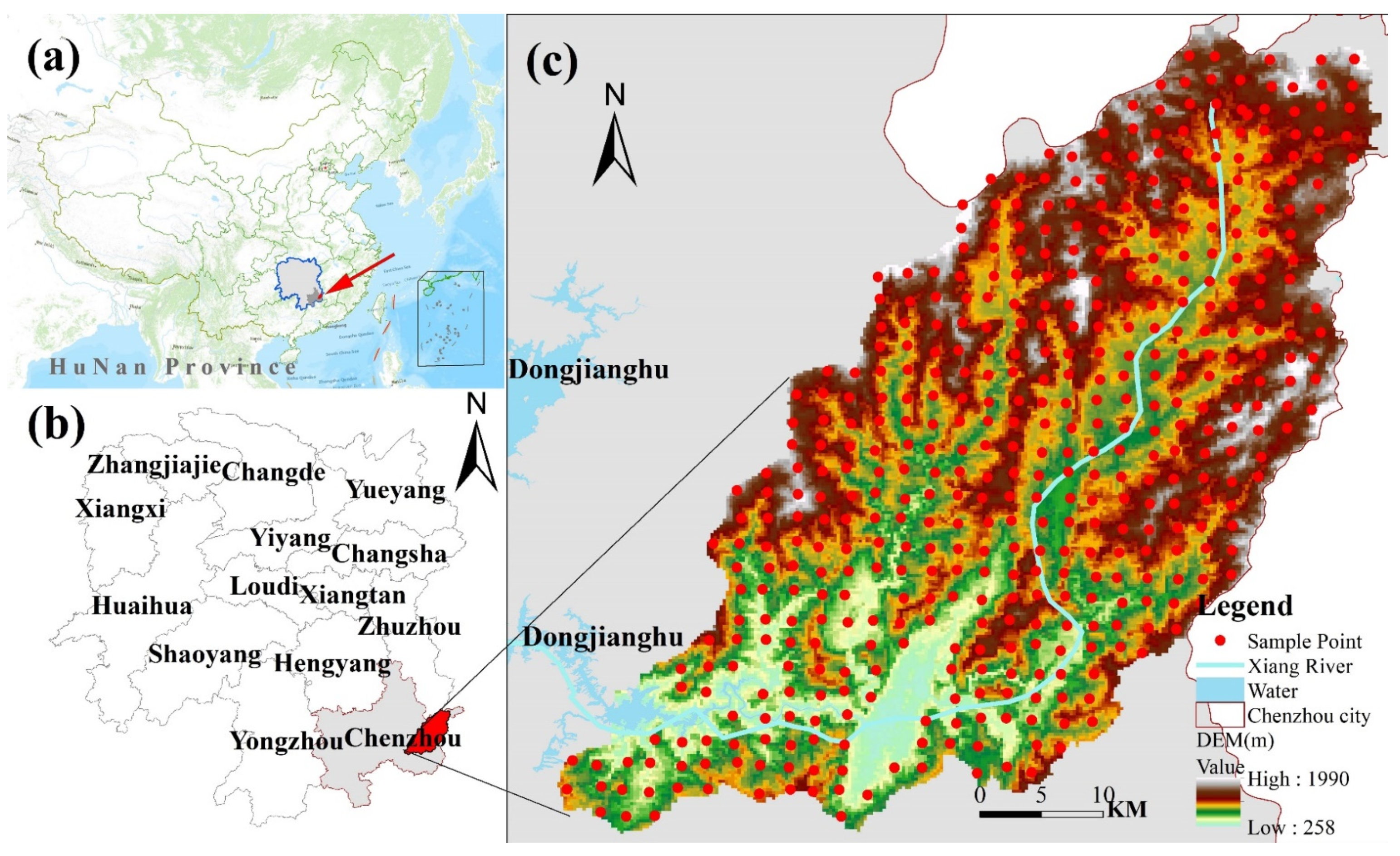
2.1. Study Area and Soil Sampling
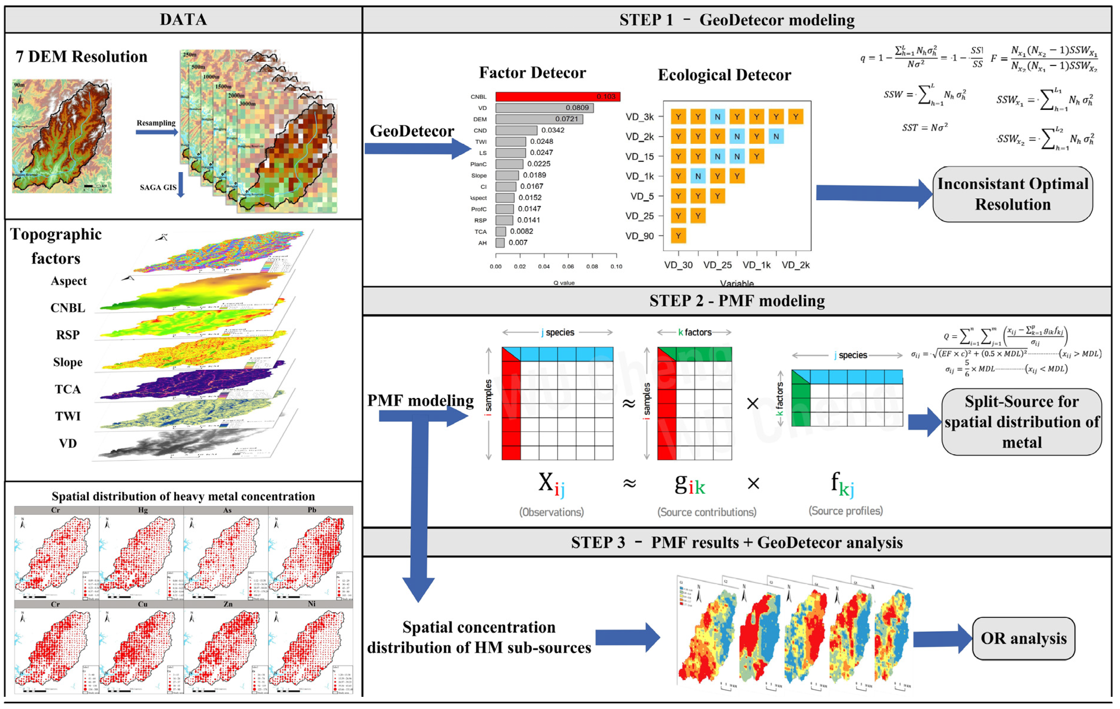
The study area (25°36′0″N–25°9′0″N, 113°27′36″E–114°1′48″E) is located in Chenzhou city, Hunan Province, China (Figure 1). Chenzhou is famous worldwide for its polymetallic deposits, and it is known as “the hometown of non-ferrous metals in the world”, with more than 143 kinds of mineral resources and over 350 million tons of polymetallic deposits reserves [32]. Intensive mining and smelting activities over decades have accumulated massive mine tailing and have caused serious soil HM pollution [33]. The study region has a sub-tropical humid monsoon climate, with an annual average temperature of 17.4 °C and annual average precipitation of 1452.1 mm. The study area is mainly dominated by a hilly topography, with a high northwest and low southeast.
A systematic grid sampling (2 × 2 km cells) was conducted in 2018, with soil samples collected from 486 sites in the study area. During field sampling, an alternative location that is close to the predesigned sites was selected to obtain natural soil in case of unavailability for sampling at the original location. At each sampling site, 5 to 6 subsamples of topsoil (0–20 cm) within a 100 m radius were collected and mixed. The mixed soil samples (1 kg) were stored in polyethylene bags and brought back to the laboratory. All soil samples were air-dried at room temperature, passed through a 2 mm polyethylene sieve, and were digested using HNO3-HClO4-HF. The concentrations of cadmium (Cd), lead (Pb), chromium (Cr), nickel (Ni), copper (Cu), and zinc (Zn) were determined by inductively coupled plasma atomic emission spectrometry (ICP-AES) with detection limits of 0.030, 2.00, 0.40, 0.30, 0.60, and 2.00 mg kg−1, respectively. Mercury (Hg) and arsenic (As) were determined by atomic fluorescence spectrometry (AFS) with detection limits of 0.010 and 0.002 mg kg−1, respectively. In addition, considering the quality control, we used duplicate samples, procedure blanks and GBW-07404 as standard reference materials, with recovery rates ranging from 93.7% to 104.5%.

2.2. Methods

In this study, all statistical analyses and calculations were conducted using R 4.1.2, and ArcGIS (Map and Pro) 10.6 was used for producing spatial distribution maps. The extraction of TFs at different resolutions was performed with SAGA GIS 8.0.1. The study route is shown in Figure 2.

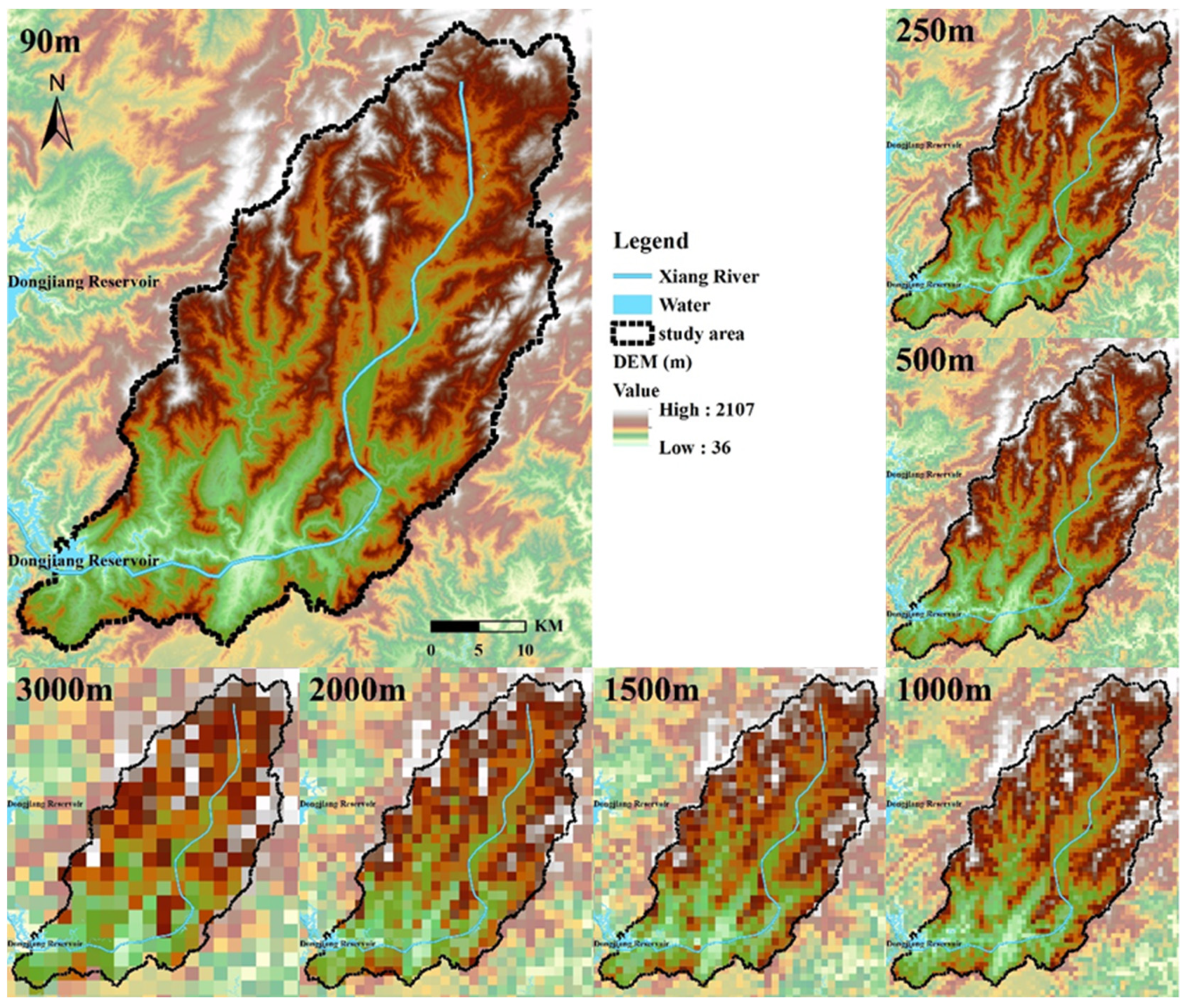
2.2.1. DEM Gradient Generation

To explore the impact of DEM resolutions on GeoDetector analysis in terms of the spatial distribution of soil HMs, a series of DEMs with various spatial resolution gradients were generated. In our study, we used the SRTM V3 dataset with 30 m resolution as the finest and basic DEM [34]. Specifically, we resampled the 30 m resolution DEM data by bilinear interpolation in ArcGIS, which has been widely used for DEM resampling in related studies [35,36,37]. Therefore, this basic DEM data were then resampled using the bilinear interpolation method to produce coarser DEMs with spatial resolutions of 90 m, 250 m, 500 m, 1000 m, 1500m, 2000 m, and 3000 m, finally forming a series of 7-level resolution gradients of DEMs (Figure 3).

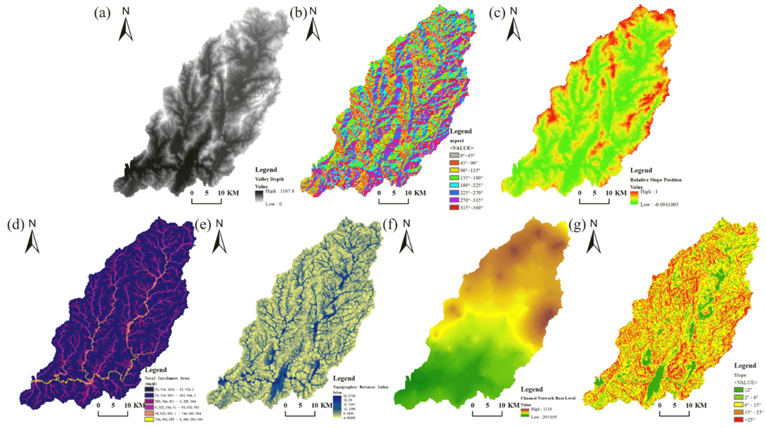
2.2.2. Topographic Factors

Based on a thorough literature review for soil HM distribution and a preliminary investigation of the study area characteristics, we determined 8 commonly used TFs for soil HM analysis and calculated them with the SAGA GIS [38]. A brief description of these factors and references to their algorithms are listed in Table 1, which mainly characterizes the topographic undulation (DEM, VD), ground roughness (Aspect, RSP), soil wetness (TCA, TWI), and others (CNBL, Slope).
Among them, TFs such as DEM (which characterize ground relief and elevation) are mainly considered to be more relevant to atmospheric deposition and soil erosion, while factors such as Aspect (which characterize surface roughness) are mainly considered to affect soil erosion and water erosion by influencing solar insolation, soil deposition, denudation flow, intensity, etc. Factors such as TWI (which characterize the degree of soil wetness, i.e., the soil water (moisture) content), are generally believed to play a role in the transport and transformation of HMs in soil water. As an aside, CNBL refers to the depth of the groundwater table, which also has an impact on the soil water content to a certain extent [39].
Figure 4 shows the TF map of the study area with a selected grid resolution of 250 m. It can be observed that certain factors have a strong continuity (e.g., CNBL, RSP), while others appear to be more random, and the corresponding distributions have obvious spatial heterogeneity (e.g., Aspect, Slope).

2.2.3. GeoDetector Model

We used the GeoDetector model to identify the influencing TFs on the spatial distribution of soil HMs. The GeoDetector model [43] consists of four sub-modules: a factor detector (FD), a risk detector, an interactive detector, and an ecological detector (ED). In this study, the FD and RD modules were primarily used. Specifically, the FD quantitatively detects the degree of interpretation of certain factors of X for the variable of interest Y (Y refers to HM soil concentration in this study). The ED is for the purpose of examining (F test) to determine whether one of the factors X1 is more influential than another factor X2.
  • Factor detector:
The FD detects the spatial heterogeneity of HM concentrations and how influencing factors explain the spatial distribution patterns of HM concentrations. The  q   v a l u e  (passed the t-test, p < 0.05) can indicate the explanatory power of individual factors on the spatial distribution of HM concentrations [43]. The  q   v a l u e   q  is calculated using the following equation:
q = 1 h = 1 L N h σ h 2 N σ 2 = 1 S S W S S T
S S W = h = 1 L N h σ h 2
S S T = N σ 2
where  h  denotes the hth  X  category out of a total of L categories;  N h  is the count of samples in category  h N  is the total number of samples across the whole study area;  S S W  is the sum of variance in category  h  in the study region;  S S T  is the sum of global variance in category h in the study region;  σ h 2  is the variances of samples in the category h; and  σ 2  is the overall variance of  Y  in the entire region, regardless of X categories.
GeoDetector can apply the significance test to  q . For  q 0,1 , a higher  q  ( p < 0.05 ) means a more substantial explanatory power of  X  on  Y , which further implies a higher influence on the spatial distribution of soil HMs.
2.
Ecological detector:
The ED is used to test if an explanatory variable X1 has a higher impact than another variable X2. The significance of the different influence of explanatory variables is tested with the F-statistic [43,44]:
F = N x 1 ( N x 2 1 ) S S W X 1 N x 2 ( N x 1 1 ) S S W X 2
S S W x 1 = h = 1 L 1 N h σ h 2
S S W x 2 = h = 1 L 2 N h σ h 2
where  N x 1  and  N x 2  represent the sample sizes of the two factors X1 and X2, respectively;  S S W X 1  and  S S W X 2  are the sums of variance in category h formed by X1 and X2, respectively; and  L 1  and  L 2  are the numbers of categories of  X 1  and  X 2 , respectively.
Thus, with a given significant level, the null hypothesis  H 0 : S S W X 1 = S S W X 2  is tested with the  F -distribution table. If the null hypothesis is rejected at the significance level of α, then there are significant differences in the effects of the two factors  X 1  and  X 2  on the spatial distribution of factor  Y .
3.
Optimal Parameters-based Geographical Detector Model (OPGD)
Given that the GeoDetector method was only able to deal with discrete variables [43], the continuous data for the 8 individual factors were first transformed into categorical data and then entered into the GeoDetector model via the optimal parameters-based geographical detector model (OPGD) [15]. The OPGD model selects the best combination of the discretization method and the break number for each geographical continuous variable as the optimal discretization parameters. A set of combinations of discretization methods (i.e., equal, natural, quantile, geometric, and standard deviation) and break numbers are provided for each continuous variable to compute the respective  q . For a continuous variable, the parameter combination with the highest  q  among all combinations is selected for spatial discretization since it presents the highest importance of the variable from the perspective of spatial-stratified heterogeneity.

2.2.4. Source Apportionment Model—Positive Matrix Factorization Model

To further analyze the natural processes hidden behind a proper resolution, the positive matrix factorization (PMF) method, a prevalent source apportionment model, was applied [45]. In PMF, a concentration data matrix  X n × m  can be factorized into contribution, profile, and residual matrices, and these are represented by  G n × p F p × m , and  E n × m , respectively. The factor contributions (G) and profile (F) are obtained by minimizing the object function ‘Q’, which is defined as follows:
Q = i = 1 n j = 1 m x i j k = 1 p g i k f k j σ i j
σ i j = E F × c 2 + 0.5 × M D L 2   x i j > M D L
σ i j = 5 6 × M D L   x i j < M D L
The matrix form of the PMF model is expressed as follows:
X n × m = G n × p · F p × m + E n × m
Equation (10) can be rewritten in the element form as follows:
x i j = k = 1 p g i k f k j + e i j
where n and m denote the numbers of samples and species, respectively;  x i j  is the measured concentration of  j t h  species in the  i t h  sample;  g i k  is the mass contribution of  k t h  factor to the  i t h  sample;  f k j  is the mass fraction of the  j t h  species from the  k t h  factor;  σ i j  is the  j t h  species’ estimated uncertainty in the  i t h  sample;  p  represents the number of extracted factors;  σ i j  represents the estimated uncertainty associated with the  j t h  species in the  i t h  sample [46];  M D L  stands for the detection limit of a specific metal species (details in Section 2.1); and  E F  denotes the error fraction, i.e., the relative standard deviation associated with the  j t h  species concentration.

3. Results and Discussion

This section may be divided into subheadings. It should provide a concise and precise description of the experimental results, their interpretation, as well as the experimental conclusions that can be drawn.

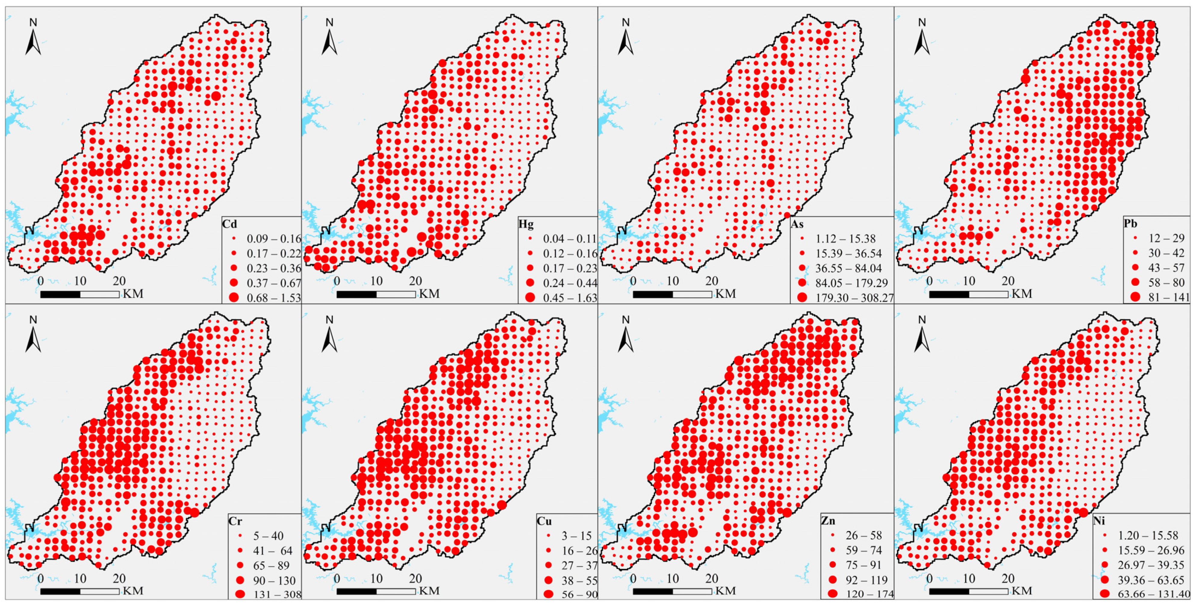
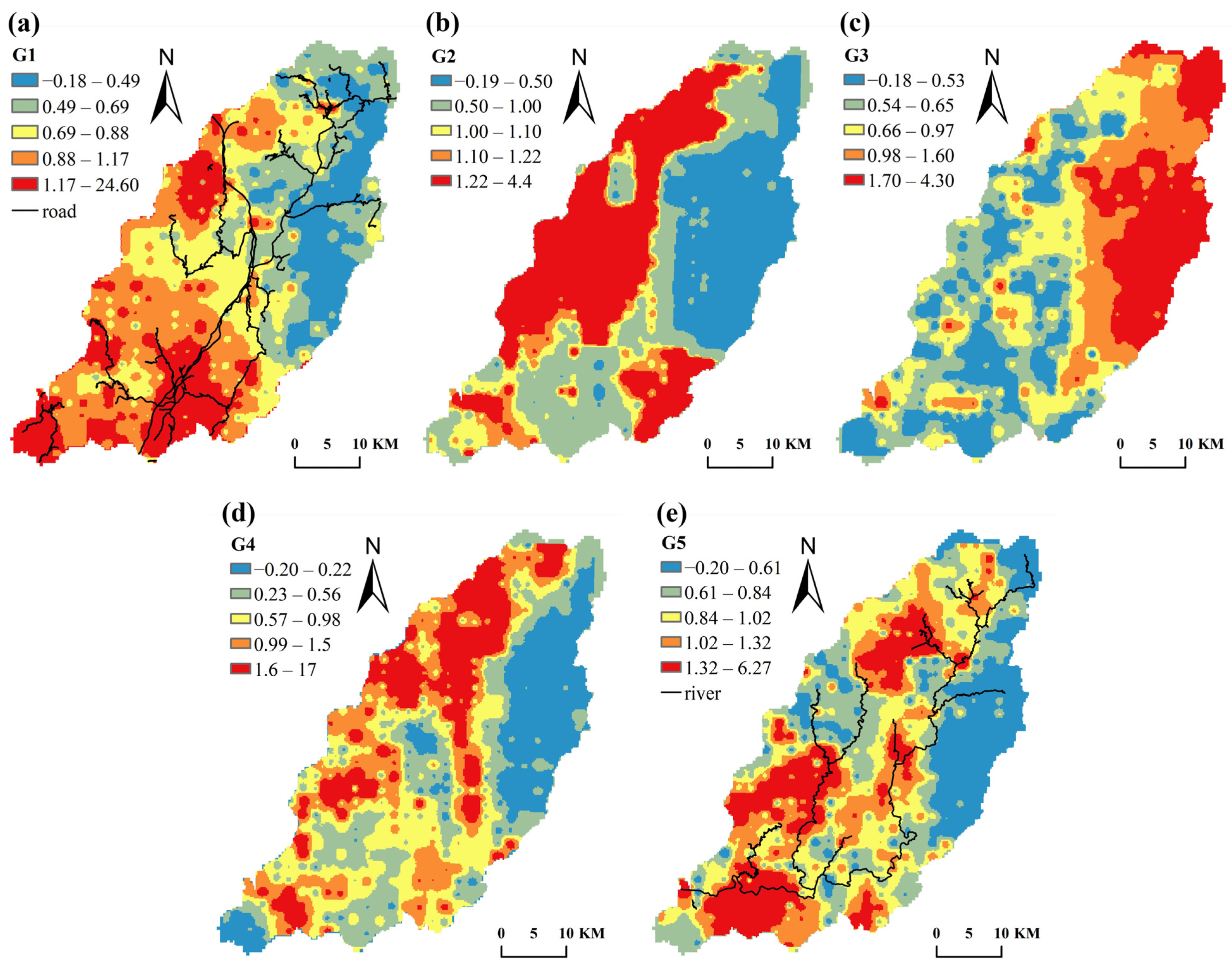
3.1. Spatial Distribution Characteristics of HMs and Topographic Factor

3.1.1. Statistics of Soil HM Concentration

The descriptive statistics of eight HMs in four hundred and eighty-six samples are summarized in Table 2. The spatial distribution of HM concentrations in the study area is shown in Figure 5. The average contents of Cr, Ni, Cu, Hg, Cd, Zn, Pb, and As were 63.13, 23.39, 27.58, 0.16, 0.21, 77.91, 39.92, and 19.14 mg kg−1, following the descending order: Cr > Pb > Cr > Cu > As > Ni > Cr > Cd > Hg. The coefficient of variation (CV) is the ratio of the standard deviation and the average, which is standardized to eliminate the dimensional influence. In general, when the CV exceeds 100%, it indicates that the HM element has strong variability; when the CV is between 10% and 100%, it indicates that the HM element has moderate variability; and when the CV is less than 10%, the HM element shows weak variability [47]. According to Table 2, the Cd, Zn, and Pb in the soil have CVs exceeding 100%, showing strong variability. In contrast, the CVs of Cr, Ni, Cu, and Hg exceeded 10%, showing moderate variability.

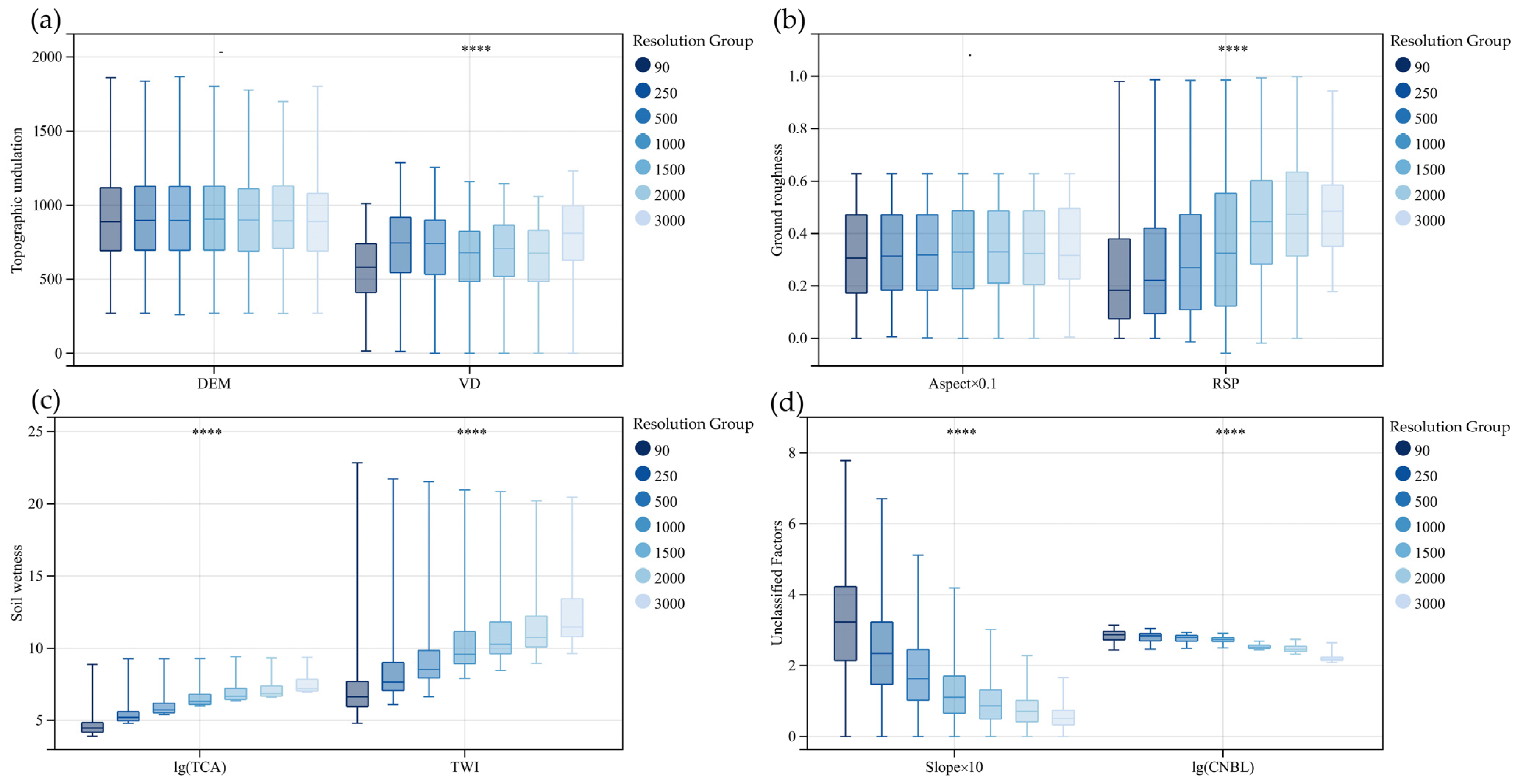
3.1.2. Topographic Factors at Different Resolutions

To investigate the effects of DEM resolution on TF, the boxplots of each TF at seven resolutions were first displayed (Figure 6). Different TFs have different responses to resolution changes. For the factors characterizing ground undulation, with the decrease in resolution, the topographic undulation gradually becomes blurred, and the difference between data tends to become less obvious and the correlation of local representative data of elevation also weakens to a certain extent. As can be seen from Figure 6a, the CNBL data tend to concentrate, and the mean value gradually decreases. With the factor characterizing ground roughness, the variance decreases near the median as the resolution decreases, as can be seen in Figure 6b. This indicates that the extracted surface roughness decreases with a coarser resolution, and the ground tends to be flat and smooth [49,50,51,52]. It appears that soil moisture factors are more consistent. The TCA significantly increases when the resolution changes from 90 m to 3000 m (Figure 6c). As the DEM resolution increases, river features of tributaries gradually fade, resulting in more areas being identified as riverbeds, which leads to an increase in the calculated area of the riverbed. These outcomes lead to more water being judged as propagating from the river unit to the surrounding land units in the topographic calculations.

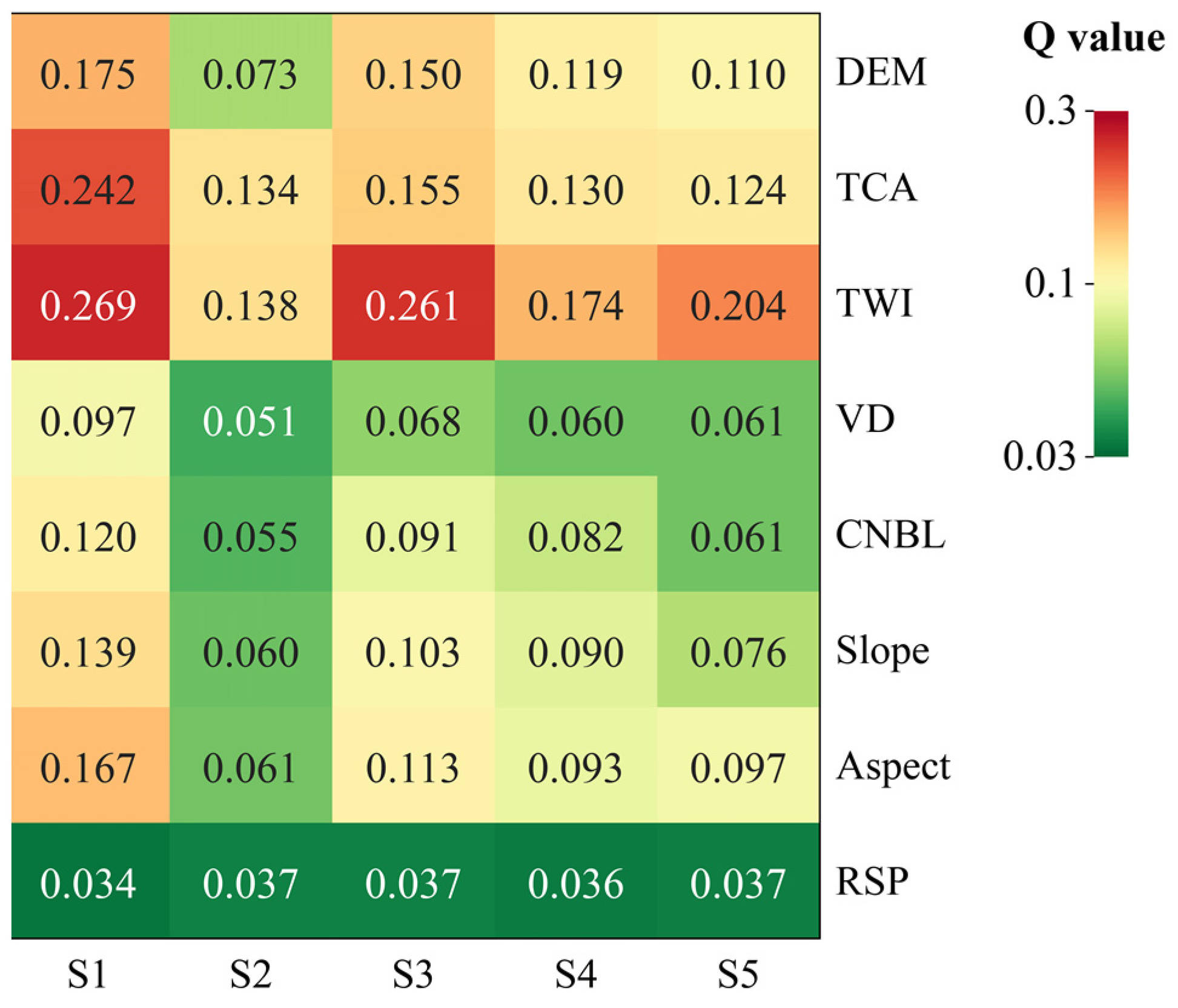
3.2. Explanatory Power of Topographic Factors at Different Resolutions Using GeoDetector

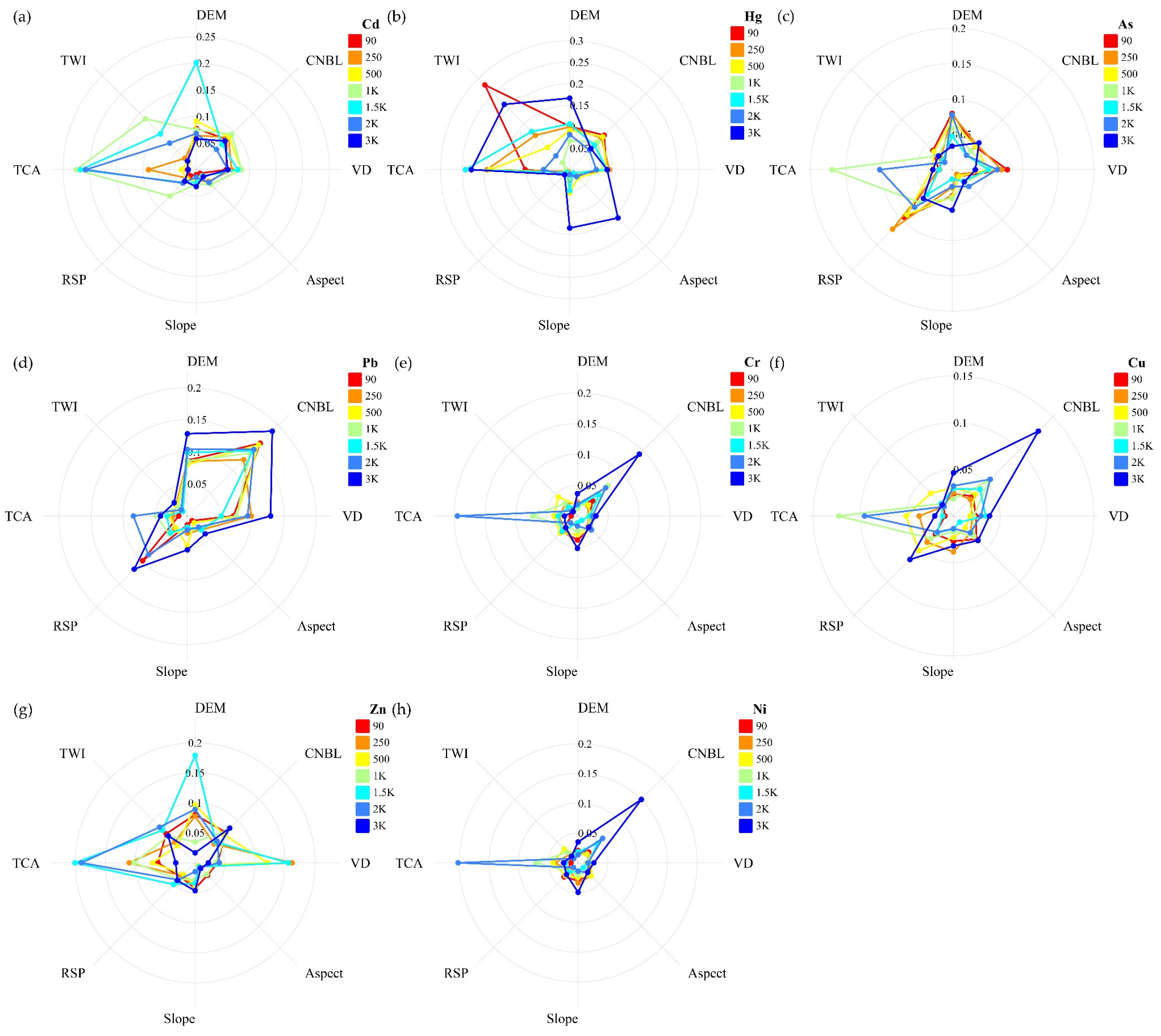
3.2.1. The Inconsistent q Results of Topographic Factors

In this section, we used the factor detection function (Section 2.2.3) of GeoDetector to characterize the interpretability of each TF on the spatial distribution of the eight HMs, and we repeated the process for all resolutions. Figure 7 shows the q of the eight TFs at seven different resolutions, with red-to-blue spectrum colors distinguishing the resolution gradient from finest (90 m) to coarsest (3000 m). Under different resolutions, the TF ranks, in terms of q values that characterize the topographic features, have significantly different explanatory power for HMs distributions, and the dominant influences obtained are also inconsistent. For example, for Hg, TWI emerged to be the dominant factor among the eight TFs at 90 m resolution, whereas TCA took the lead at 3000 m resolution. Such inconsistency is also found in other HMs. In addition, the HMs (Cr, Ni, and Cu) with less human activity impacts (discussed in Section 3.1.1) had good consistency in q distribution, and the corresponding q values were smaller and more concentrated than those of HMs with high human influence (Figure 7e,f,h). However, the value of the specific q, that is, the interpretation degree of the spatial distribution of HMs, was found to be different. We also noted that the influence of the CNBL factor was the largest for all HMs, suggesting that groundwater plays a pivotal role in interpreting the distribution of soil HMs.
To summarize, it is evident that factor detection with different DEM resolutions produces inconclusive and contradicting results. This implies that previous studies that used GeoDetector to analyze environmental factors at a specific resolution may be biased. In other words, the detection results obtained from the unrefined selected resolution may not be tenable, which may lead to questions about the scientific validity and reliability of certain conclusions [5,8,17]. Therefore, it is necessary to select the most appropriate resolution, or to at least further analyze the impacts of the resolution.

3.2.2. Test of an Optimal Resolution for Each Topographic Factor

As discussed above, the ability of TFs to interpret the distribution of HMs considerably varies at different resolutions. We hypothesized that each TF requires a proper DEM resolution so as to embody its involvement in certain HM migration processes that may occur or only be identified at certain spatial scales. We explored whether there is an OR for each TF that provides the strongest interpretation. With the TF detection results for each HM, we chose the resolution with the highest q for each HM as the OR. In order to account for the inaccuracies along the discretized resolution gradient, ED was applied to test whether the q of a certain resolution differed from the highest q, and the resolutions that were insignificantly different from the highest q (p ≥ 0.05) were also regarded as the best resolutions.
As shown in Table 3, there is no uniform OR for a TF across all eight HMs. For each TF, each HM has its preferred resolution. However, we found that some HMs with similar properties show consistency in terms of OR. For example, the ORs for three HMs (Cr, Ni, and Cu), which are less affected by humans, were almost the same. However, the remaining metals were not always consistent. Such inconsistencies strongly suggest that one TF may exert effects in multiple HM migration processes and exhibits an influence at multiple spatial scales. In light of the environmental knowledge that each metal has its characteristic source and physicochemical governing laws when migrating in an environmental system that crosses various environmental media, it will be pertinent to probe the underlying sources of HMs and to conduct a subsequent GeoDetector analysis on the identified HM sources (which are elaborated in the following Section 3.3).

3.3. Possible Explanation for the Inconsistency of the Optimal Resolution

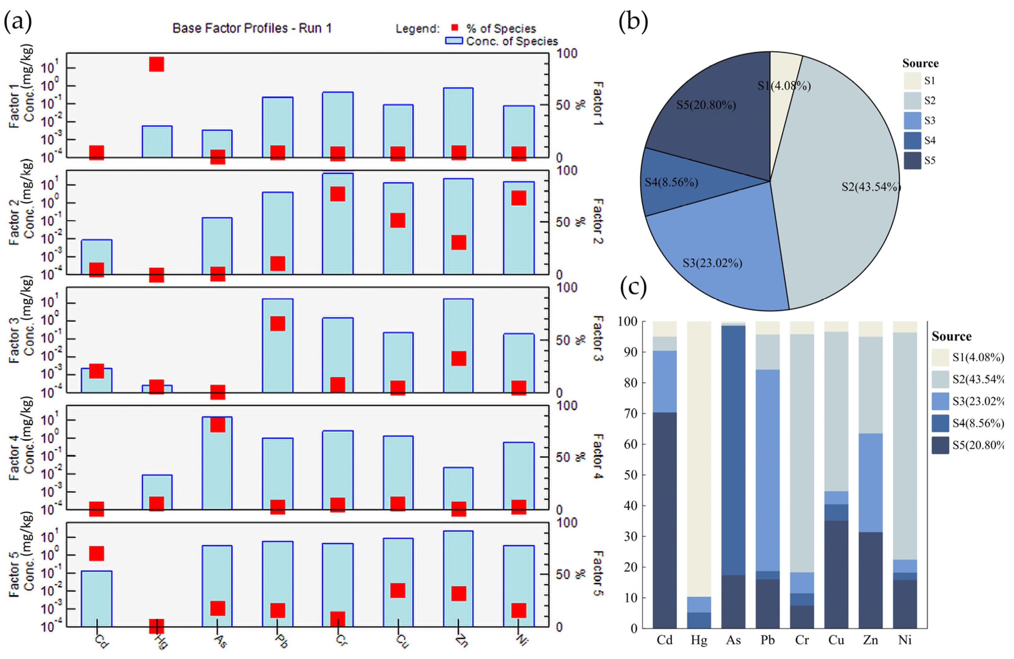
3.3.1. The Source Appointment of Soil HMs Using PMF

To explore the possible reasons for inconsistent ORs, the PMF model was applied to identify the HM sources and underlying environmental processes (Table S1 in Supplementary Materials). After comparing four- to six-source configurations (Table S2 in Supplementary Materials), we found that the four-source solution was insufficient in achieving the required level of simulation. The six-source solution led to ostensibly better observation-to-prediction correspondence; however, this was at the cost of the sources’ stability. Thus, the five-source solution was finally selected for further analysis, as was suggested by error estimation diagnostics. We identified the sources based on the major metals in the source profiles (Table S3 in Supplementary Materials) in combination with the spatial distribution of the source contribution data (G matrix, Figure 8a) after spatial interpolation. The blue boxes in Figure 8a indicate the concentration of each HM attributable to each source (i.e., source profiles), and the red squares indicate the percentage of each HM attributable to each source. Figure 8b shows the proportion of five PMF sources in terms of the average contribution of the eight HMs. Figure 8c shows the concentration (in percent) of each HM, and their contributions to each source are displayed as stacked bars in the Factor Fingerprints screen.
Source 1 (S1) accounts for 4.1% of the total concentration, and it has Hg as the main loading element, accounting for 89.6% of the total Hg source. The rest of the HM loadings were not high in S1. The high CV of Hg (Table 2) indicates a high human activity influence. Over the past decades, coal combustion has been the largest source of atmospheric Hg emissions, especially in China [53], where coal combustion accounts for more than 60% of total emissions [54,55]. During coal combustion, almost 100% of the Hg is transmitted to the flux gas, including gaseous elemental Hg, gaseous oxidized Hg, and particulate-bound Hg. Among them, gaseous elemental Hg is not easily captured and escapes into the atmosphere due to its insolubility [56]. Vehicle emission is another important Hg source [57,58] as it can be seen that S1 hotspots are mainly distributed near main roads with heavy traffic (Figure 9a). Thus, atmospheric and soil moisture is an important factor influencing Hg fate and transport. In addition, since the soluble Hg content in soil is low and mostly accumulates in the surface layer of the soil, it is more sensitive to soil properties such as organic matter content and TFs such as altitude, surface roughness, etc. In summary, S1 is considered as the atmospheric emissions, and the associated deposition and transport (Figure S1 in Supplementary Materials).
Source 2 (S2) accounts for 43.5% of the total concentration, with Cr, Ni, Cu, and Zn being the major loading elements, accounting for 77.5%, 73.9%, 51.9%, and 31.5% of the total sources, respectively. Previous studies have shown that parent material is the main source of Cr and Ni in Hunan, China [59]. Moreover, the Cr and Ni in soil are typically considered as natural origin in Guangdong, China [60], and in Ahvaz, Iran [61]. The CVs of these four HMs were all less than 0.6, indicating relatively small spatial variability. Furthermore, the G2 spatial distribution (Figure 9b) maps the lithology fairly well (Figure S2 in Supplementary Materials), thus corroborating this natural source interpretation. The mica-like minerals enriched in siliciclastic sedimentary rocks are strongly adsorbed to Cr, Ni, REE (Rare Earth Element), and PGE (Platinum Group Elements), acting as concentrators and aggregators for the elements [62,63]. In acid plutonics, the Cr and Ni tend to form acidic compounds after high oxidation, and they consequently become mobile rather than stay fixed in the lithological layers [64], as evidenced by the cold spots presented in Figure 9b. Therefore, the content distribution of the Cr and Ni in this region are largely related to this geochemical property. In summary, S2 is treated as a natural source in the soil-forming parent material, and it is mainly closely related to the properties of the soil itself.
Source 3 (S3) accounts for 23.0% of the total concentration, and Pb (65.6%), Zn (32.1%), and Cd (20.1%) were the dominant metals in this source. Our research area was located in the mineral-rich region of China and has seen intensive mining and smelting activities that date back through a long history of non-ferrous metal mining, beneficiation, smelting, and trading [65]. As shown in the G3 map (Figure 9c), the concentrations of Pb, Cd, and Zn are mainly distributed around mining and smelting plants, forming multiple radially divergent concentration gradients of Pb, Cd, and Zn (Figure S3 in Supplementary Materials). Through field research, the eastern part of this study area is rich in minerals of galena (PbS) and sphalerite (ZnS), and the Pb and Zn have heavily invaded the surrounding soil environment during the mining and smelting process. Furthermore, Cd is an associated element (it is positively correlated with the content of these trace elements that cause the color change in sphalerite and is able to synchronously enter the lattice of sphalerite [66]), thus its concentration is also much higher than the background value. Industrial and mining pollution mainly comes from mining, ore smelting, mine wastewater discharge, slag piles, tailings, leaching, etc. HMs enter the mine soil through dust fall, leaching, and residue [67]. To summarize, S3 is mainly a source of HM mine dust pollution generated by industrial activities.
Source 4 (S4) accounted for 8.6% of the total concentration, with As being the leading element that represented 81.1% of the total arsenic source. For four centuries, due to the abundant arsenic sulfide ore resources in Chenzhou, the workshop form of arsenic metallurgy involved using an indigenous method, which is the mainstream of the local export process [68]. This continued until the famous arsenic poisoning case in 2006, when this periodic small-point source but large-scale and long-term uncontrolled anthropogenic activity was gradually extinguished (http://www.hunan.gov.cn/hnszf/xxgk/yjgl/dxal/201301/t20130108_4694347.html, accessed on 1 July 2023). However, due to the low solubility of As, most of the pollutants containing As are adsorbed by soil colloids after entering the soil. This mainly occurred in an adsorbed state, which accumulated in the surface layer of the soil and is difficult to vertically seep. Therefore, the As was separated out as a single source (Figure S4 in Supplementary Materials), and S4 was considered to be the historical anthropogenic contamination of As.
Source 5 (S5) is the fifth source (F5). It accounted for 20.8% of the total concentration, and Cd was the main contributing element, which accounted for 70.3% of the total Cd source. Meanwhile, Cu and Zn also accounted for a larger proportion of this source at 35.2% and 31.4%, respectively. The CVs of these three HMs were all less than 0.66, indicating a smaller spatial variability and less anthropogenic influence. The spatial overlap with the S2 also proved the natural qualities of this source. Cd, Cu, and Zn all have substantial species as dissolved cations or chelated cations in the soil moisture; therefore, they become similar to each other to a certain extent [69,70]. Furthermore, we all know that the three HMs, Cd, Cu, and Zn, increase in solubility as pH decreases, as was corroborated by the spatial correspondence between their concentrations and soil pH (Figure S5 in Supplementary Materials). In addition, it can be seen that the distribution of this source is concentrated at the dense intersection of river networks (Figure 7e, G5), the hotspots are mainly clustered at the confluence of the river network and its downstream, and the concentration is not high at the upstream source. Therefore, S5 is interpreted as a hydrological process driven by the natural source.

3.3.2. Different Sources (Processes) Lead to Inconsistent Optimal Resolution Results

Based on the above analysis, we found that the PMF not only distinguishes the pollution sources, but also more precisely divides the different formation processes of soil HM distribution, including pollution sources, pollution transformation, and pollution transport processes. In this study, the general term “source” is used in all instances where the distinction between “source” and “source and process” is considered non-critical. Combining the results of the source apportionment calculated above, we further used the PMF-modeled concentrations attributed to the five sources for the detection of the influential TF at 90–3000 m resolution. As detailed in Section 3.2.2, we processed the FD and ED of the GeoDetector model in sequence to select the best resolution corresponding to the maximum q value, or for the resolution that was not significantly different from the maximum q value. Due to the linear allocation principle in the PMF, the OR of the HMs for the same source at each resolution show complete consistency. Therefore, for the sake of brevity, we no longer distinguish between the different HMs and display them together by source (Table 4). Additionally, the largest q values that were filtered by the t-test (p < 0.05, FD) and F-test (p > 0.05, ED) of the GeoDetector model are shown in Figure 10. When comparing the q values and their sorts of the TFs for the total HMs obtained in Section 3.2.1, the results of source-specific HMs show a large difference (Figure S6 in Supplementary Materials), which indicates the effects of pollution sources (processes) on the OR detections of the TFs.
The Hg in the soil is mainly attributed to the S1 source, which accounts for 89.6% of the total Hg content. Thus, it is reasonable that the ORs of S1 and the Hg shows a good consistency (Table 3 and Table 4).
The Hg in the soil is mainly attributed to the S1 source, which accounts for 89.6% of the total Hg content. Thus, it is reasonable that the ORs of S1 and the Hg show good consistency (Table 3 and Table 4). S1 reflects the whole processes of atmospheric emissions, transport, as well as the deposition of Hg in three major forms: gaseous elemental Hg, gaseous oxidized Hg, and particulate-bound Hg. On the one hand, gaseous elemental Hg quickly moves with the wind, and geographical factors related to atmospheric dispersion favor larger scales or coarser resolutions. These factors include DEM and Aspect. On the other hand, the gaseous oxidized Hg and particulate-bound Hg have higher deposition velocities and are much more easily washed out by precipitation [69]. Therefore, geographical factors that are involved in atmospheric deposition—wet or dry—may favor small scales or finer resolutions. The factors of TWI, TCA, and CNBL that were obtained with finer resolutions may emerge as significant drivers; nonetheless, these factors obtained with coarser resolutions should not necessarily become dimmed because land surface features may also exist at large scales. There may be complex reasons that the groundwater level (CNBL) and soil moisture (TWI) factors stand out as Hg concentration drivers. One possible explanation is that the water in soil and the related groundwater in certain cases manifest the sensible heat flux of the soil, and the heat that may hence be available for soil Hg volatilization. Another plausible explanation is that these two factors are indirect surrogates of the precipitation prevalence and, hence, the airborne Hg wet deposition.
Due to the existence of a dominant source, with S4 representing 81.1% of the total As, the ORs of As agree well with the ORs of S4 (Table 3 and Table 4). Based on the historical anthropogenic pollution activities described in the previous section, this kind of periodic small point source with widespread, and uncontrolled pollution processes and local characteristics, more refined geographical factors may better reflect the extensive and intensive contaminations. A larger scale may not be sufficient enough to portray this frequent and dense small-point source pollution. The finer OR performance in Table 4 also proves this sentiment.
A similar situation also occurs for Pb. S3 (the industrial mining pollution process) contributes to 65.6% of the total Pb. Thus, the OR preference of Pb could be well explained by the OR preference of S3 (Table 3 and Table 4). The distance over which mineral dust is transported depends on the transporting winds and settling velocities determined by the particle characteristics including size, shape, and density [70]. The Pb in S3 differs from the Hg in S1 in terms of nonvolatility and particle size. Compared to gaseous metal, metals such as Pb in S3 are adsorbed on the mineral dust (large particles) released by mining activities, which have a higher settling rate and are therefore deposited closer to the pollution source. As the atmospheric deposition of dust is critically determined by the gravitational force rather than the atmospheric hydrodynamic resistance or the land surface characteristics, the land topography or landcover type varieties that critically appear at finer resolutions are rendered insignificant, and this is also witnessed by the large ORs at 2 km or 3 km (Table 4).
Due to the multiple sources of the remaining HMs (i.e., Cr, Cu, Ni, Cr, Cd), their ORs also reflect the integrated effects of related sources and processes. For example, the total Zn was composed of S2 (31.5%), S3 (32.1%), and S5 (31.4%). The soil parent material (S2) and its OR are mainly determined by the spatial range of lithological classes. The milder variation of lithology in the space will render TFs that reflect large-scale characteristics, which are readily identifiable as significant drivers. Factors such as CNBL and TCA, which respond to the overall watershed division of the region and hence readily stand out with coarser resolutions, are then “detected” by GeoDetector (Table 4). Moreover, S5 was identified as the natural source that is driven by hydrological process, evidenced by the spatial correspondence with the river network distribution and soil pH. Thus, it is unsurprising that the TFs that indicate “water” in a certain sense, such as TCA, CNBL, and TWI, all stand out as significant drivers of S5. The partial amount of Zn from S5 in the soil may undergo speciation processes depending on the fluctuation of soil Eh and soil moisture, which is further governed by solar radiation, runoff/flooding seasonally changes, etc. Thus, the TFs that exert an influence on solar radiation and runoff/flooding will emerge as significant factors. These factors include Aspect, DEM, Slope, VD, etc. Generally, hydrological processes and associated metal speciation will not be as rapid as atmospheric dispersion/deposition; consequently, S5 metals will be mostly sensitive to the factors that are obtained with medium-to-large spatial resolutions.
In summary, our analysis denies the existence of an optimal DEM resolution for the TFs among the HMs. The main reason for the inconsistent OR is that each HM may have various sources and subsequent environmental processes that occurred at different spatial scales. Moreover, each TF could also simultaneously reflect the different environmental processes. Therefore, the apparent OR for one metal is jointly composed of the preferences for all the sources it contains, and thus it cannot be determined by the OR preferences of a single source alone. Although the GeoDetector developers have already raised the issue of spatial scale with three cases (i.e., spatial raster data, spatial point data, and areal statistical data) [15]; most previous studies still used experience to determine the scale (resolution) rather than quantitative assessments, which may have led to biases in the results [19,20]. To address this issue, this study investigated the DEM resolution effects of GeoDetector detection from the source perspective, and proposed three scenarios and strategies for selecting the best resolution for a more robust GeoDetector analysis:
  • Strategy 1 is applicable to the scenario in which the dominant pollution source is well known, such as the Hg and As in this study. By jointly analyzing the physicochemical properties of Hg and As, and the corresponding sensitivity factors for the source and process, the possible OR of the factors can be effectively determined.
  • Strategy 2 is for scenarios where the HM’s sources and corresponding processes are known but they are level-pegged. For example, Cr is the main HM in both S2 and S5 in this study, thus its OR performance is jointly composed of the preferences of all the sources it contains, and thus cannot be determined by the OR preferences of a single source alone. Strategy 2 is also applicable to scenarios where one specific TF differs in its representation of sources and processes at different spatial scales. Such an example can be found in the TWI for Hg in S1 and Pb in S3. A fine-scale TWI may be more conducive to highlighting flexible processes such as atmospheric deposition sources and accompanying soil transport, while large-scale TWI may be able to adequately characterize mineral dusts and their subsequent transport. In these cases, further comparison and evaluation at different resolutions should be conducted before GeoDetector analysis.
  • Strategy 3 is mainly suitable for scenarios where pollution source analysis is not available, as was the case in most previous studies. We recommend trying at least several different resolutions to select the most explanatory resolutions possible.

4. Conclusions

In this study, we investigated the effects of DEM resolutions on identifying the driving TFs of soil HMs when using GeoDetector. We demonstrated that TF detection at different resolutions leads to inconsistently important sorting, which may affect the scientific validity of the conclusions. However, there is no uniform OR for each TF. Using the source apportionment PMF, we found that the different sources of HMs and the accompanying transport and transformation processes are the main reasons for such OR inconsistency. To identify the appropriate resolution for specific studies, we presented alternative strategies for three scenarios with ad hoc considerations of the composition and intensity of pollution sources. Where pollution source analysis is not available, it is recommended to try at least several resolutions to determine the most explanatory resolution. The investigations in this study investigate the issues of DEM resolution effects and pollution sources in identifying the driving TFs of the soil HM distribution, and these findings could help inform a more robust GeoDetector analysis. Additionally, the generalizability of these results is subject to certain limitations since we selected a typical polluted area with limited environmental conditions. Hence, further research is needed to validate the results using data from other areas with different meteorological, geological, and hydrological characteristics.

Supplementary Materials

The following supporting information can be downloaded at: https://www.mdpi.com/article/10.3390/rs15164067/s1, Table S1: Summary of EPA PMF 5.0 settings; Table S2: Summary of PMF and Error estimation diagnostics of the soil HM data; Table S3: Factor Profiles (conc. of HMs) from Base Run of the minimum dQmax (5-factors solution); Figure S1: (a) The DEM distribution (90m) and (b) Factor contribution of source 1 (identified as atmospheric emissions and subsequent deposition and transport); Figure S2: A comparison between (a) the lithology map (Hartmann and Moosdorf, 2012) and (b) factor contribution of source 2 (identified as natural source of parent material); Figure S3: A comparison between (a) distance map of the industrial sites and (b) factor contribution of source 3 (identified as pollution by industrial activities); Figure S4: A comparison between (a) concentration of As and (b) factor contribution of source 4 (identified as historical anthropogenic As contamination); Figure S5: A comparison between (a) The pH distribution and (b) factor contribution of source 5 and River Network (identified as dissolved HM soil hydrological transports); Figure S6: The factor detector results of HMs concentration after PMF source separation: (a) Source 1, atmospheric emissions and subsequent deposition and transport, (b) Source 2, natural source of parent material, (c) Source 3, pollution by industrial activities, (d) Source 4, historical anthropogenic As contamination (e) Source 5, dissolved HM soil hydrological transports.

Author Contributions

Conceptualization: Y.W. and L.Z.; methodology: Y.W. and L.Z.; software: Y.W., L.Z. and Y.M.; formal analysis: Y.W., L.Z. and Y.M.; writing—original draft preparation: Y.W. and L.Z.; writing—review and editing: Y.W., L.Z., Y.M., Q.L. and Y.F.; funding acquisition, L.Z. All authors have read and agreed to the published version of the manuscript.

Funding

This research was funded by the National Natural Science Foundation of China, grant number 42107425.

Data Availability Statement

Not applicable.

Conflicts of Interest

The authors declare no conflict of interest.

References

  1. O’Connor, D.; Hou, D. More Haste, Less Speed in Replenishing China’s Groundwater. Nature 2019, 569, 487. [Google Scholar] [CrossRef] [PubMed]
  2. Chen, T.; Chang, Q.; Liu, J.; Clevers, J.G.P.W.; Kooistra, L. Identification of Soil Heavy Metal Sources and Improvement in Spatial Mapping Based on Soil Spectral Information: A Case Study in Northwest China. Sci. Total Environ. 2016, 565, 155–164. [Google Scholar] [CrossRef] [PubMed]
  3. Hu, B.; Shao, S.; Ni, H.; Fu, Z.; Hu, L.; Zhou, Y.; Min, X.; She, S.; Chen, S.; Huang, M.; et al. Current Status, Spatial Features, Health Risks, and Potential Driving Factors of Soil Heavy Metal Pollution in China at Province Level. Environ. Pollut. 2020, 266, 114961. [Google Scholar] [CrossRef]
  4. Wu, J.; Li, J.; Teng, Y.; Chen, H.; Wang, Y. A Partition Computing-Based Positive Matrix Factorization (PC-PMF) Approach for the Source Apportionment of Agricultural Soil Heavy Metal Contents and Associated Health Risks. J. Hazard. Mater. 2020, 388, 121766. [Google Scholar] [CrossRef] [PubMed]
  5. Xiang, M.; Li, Y.; Yang, J.; Lei, K.; Li, Y.; Li, F.; Zheng, D.; Fang, X.; Cao, Y. Heavy Metal Contamination Risk Assessment and Correlation Analysis of Heavy Metal Contents in Soil and Crops. Environ. Pollut. 2021, 278, 116911. [Google Scholar] [CrossRef]
  6. Khosravi, K.; Rezaie, F.; Cooper, J.R.; Kalantari, Z.; Abolfathi, S.; Hatamiafkoueieh, J. Soil Water Erosion Susceptibility Assessment Using Deep Learning Algorithms. J. Hydrol. 2023, 618, 129229. [Google Scholar] [CrossRef]
  7. Zhao, M.; Wang, H.; Sun, J.; Tang, R.; Cai, B.; Song, X.; Huang, X.; Huang, J.; Fan, Z. Spatio-Temporal Characteristics of Soil Cd Pollution and Its Influencing Factors: A Geographically and Temporally Weighted Regression (GTWR) Method. J. Hazard. Mater. 2023, 446, 130613. [Google Scholar] [CrossRef]
  8. Sun, X.; Zhang, L.; Lv, J. Spatial Assessment Models to Evaluate Human Health Risk Associated to Soil Potentially Toxic Elements. Environ. Pollut. 2021, 268, 115699. [Google Scholar] [CrossRef]
  9. Hudson-Edwards, K. Tackling Mine Wastes. Science 2016, 352, 288–290. [Google Scholar] [CrossRef]
  10. Zhou, L.; Zhao, X.; Teng, M.; Wu, F.; Meng, Y.; Wu, Y.; Byrne, P.; Abbaspour, K.C. Model-Based Evaluation of Reduction Strategies for Point and Nonpoint Source Cd Pollution in a Large River System. J. Hydrol. 2023, 622, 129701. [Google Scholar] [CrossRef]
  11. Thompson, J.A.; Bell, J.C.; Butler, C.A. Digital Elevation Model Resolution: Effects on Terrain Attribute Calculation and Quantitative Soil-Landscape Modeling. Geoderma 2001, 100, 67–89. [Google Scholar] [CrossRef]
  12. Fang, S.; Jia, X.; Qian, Q.; Cui, J.; Cagle, G.; Hou, A. Reclamation History and Development Intensity Determine Soil and Vegetation Characteristics on Developed Coasts. Sci. Total Environ. 2017, 586, 1263–1271. [Google Scholar] [CrossRef] [PubMed]
  13. Fei, X.; Christakos, G.; Xiao, R.; Ren, Z.; Liu, Y.; Lv, X. Improved Heavy Metal Mapping and Pollution Source Apportionment in Shanghai City Soils Using Auxiliary Information. Sci. Total Environ. 2019, 661, 168–177. [Google Scholar] [CrossRef] [PubMed]
  14. Lv, J. Multivariate Receptor Models and Robust Geostatistics to Estimate Source Apportionment of Heavy Metals in Soils. Environ. Pollut. 2019, 244, 72–83. [Google Scholar] [CrossRef]
  15. Song, Y.; Wang, J.; Ge, Y.; Xu, C. An Optimal Parameters-Based Geographical Detector Model Enhances Geographic Characteristics of Explanatory Variables for Spatial Heterogeneity Analysis: Cases with Different Types of Spatial Data. GISci. Remote Sens. 2020, 57, 593–610. [Google Scholar] [CrossRef]
  16. Huang, S.; Xiao, L.; Zhang, Y.; Wang, L.; Tang, L. Interactive Effects of Natural and Anthropogenic Factors on Heterogenetic Accumulations of Heavy Metals in Surface Soils through Geodetector Analysis. Sci. Total Environ. 2021, 789, 147937. [Google Scholar] [CrossRef]
  17. Qiao, P.; Yang, S.; Lei, M.; Chen, T.; Dong, N. Quantitative Analysis of the Factors Influencing Spatial Distribution of Soil Heavy Metals Based on Geographical Detector. Sci. Total Environ. 2019, 664, 392–413. [Google Scholar] [CrossRef]
  18. Shi, T.; Hu, Z.; Shi, Z.; Guo, L.; Chen, Y.; Li, Q.; Wu, G. Geo-Detection of Factors Controlling Spatial Patterns of Heavy Metals in Urban Topsoil Using Multi-Source Data. Sci. Total Environ. 2018, 643, 451–459. [Google Scholar] [CrossRef]
  19. Qiao, Y.; Wang, X.; Han, Z.; Tian, M.; Wang, Q.; Wu, H.; Liu, F. Geodetector Based Identification of Influencing Factors on Spatial Distribution Patterns of Heavy Metals in Soil: A Case in the Upper Reaches of the Yangtze River, China. Appl. Geochem. 2022, 146, 105459. [Google Scholar] [CrossRef]
  20. Liu, Z.; Fei, Y.; Shi, H.; Mo, L.; Qi, J. Prediction of High-Risk Areas of Soil Heavy Metal Pollution with Multiple Factors on a Large Scale in Industrial Agglomeration Areas. Sci. Total Environ. 2022, 808, 151874. [Google Scholar] [CrossRef]
  21. Muthusamy, M.; Casado, M.R.; Butler, D.; Leinster, P. Understanding the Effects of Digital Elevation Model Resolution in Urban Fluvial Flood Modelling. J. Hydrol. 2021, 596, 126088. [Google Scholar] [CrossRef]
  22. Qiao, P.; Dong, N.; Lei, M.; Yang, S.; Gou, Y. An Effective Method for Determining the Optimal Sampling Scale Based on the Purposes of Soil Pollution Investigations and the Factors Influencing the Pollutants. J. Hazard. Mater. 2021, 418, 126296. [Google Scholar] [CrossRef] [PubMed]
  23. Sørensen, R.; Seibert, J. Effects of DEM Resolution on the Calculation of Topographical Indices: TWI and Its Components. J. Hydrol. 2007, 347, 79–89. [Google Scholar] [CrossRef]
  24. Tang, G.; Zhao, M.; Li, T.; Liu, Y.; Xie, Y. Modeling Slope Uncertainty Derived from DEMs in Loess Plateau. Acta Geol. Sin. 2003, 58, 824–830. (In Chinese) [Google Scholar] [CrossRef]
  25. Zhou, Q.; Liu, X. Analysis of Errors of Derived Slope and Aspect Related to DEM Data Properties. Comput. Geosci. 2004, 30, 369–378. [Google Scholar] [CrossRef]
  26. López-Vicente, M.; Álvarez, S. Influence of DEM Resolution on Modelling Hydrological Connectivity in a Complex Agricultural Catchment with Woody Crops: Modelling Hydrological Connectivity in Woody Crops. Earth Surf. Process. Landf. 2018, 43, 1403–1415. [Google Scholar] [CrossRef]
  27. Wu, Y.; Cheng, H. Monitoring of Gully Erosion on the Loess Plateau of China Using a Global Positioning System. CATENA 2005, 63, 154–166. [Google Scholar] [CrossRef]
  28. Zhang, J.X.; Chang, K.; Wu, J.Q. Effects of DEM Resolution and Source on Soil Erosion Modelling: A Case Study Using the WEPP Model. Int. J. Geogr. Inf. Sci. 2008, 22, 925–942. [Google Scholar] [CrossRef]
  29. Ariza-Villaverde, A.B.; Jiménez-Hornero, F.J.; Gutiérrez De Ravé, E. Influence of DEM Resolution on Drainage Network Extraction: A Multifractal Analysis. Geomorphology 2015, 241, 243–254. [Google Scholar] [CrossRef]
  30. Saksena, S.; Merwade, V. Incorporating the Effect of DEM Resolution and Accuracy for Improved Flood Inundation Mapping. J. Hydrol. 2015, 530, 180–194. [Google Scholar] [CrossRef]
  31. Li, M.; Zhao, Y.; Gao, G.; Ding, G.; Yu, N. Effects of DEM Resolution on the Accuracy of Topographic Factor Derived from DEM. Sci. Soil Water Conserv. 2016, 14, 15–22. (In Chinese) [Google Scholar]
  32. Zhang, J.G.; Chen, H.S.; Su, Y.R.; Kong, X.L.; Zhang, W.; Shi, Y.; Liang, H.B.; Shen, G.M. Spatial Variability and Patterns of Surface Soil Moisture in a Field Plot of Karst Area in Southwest China. Plant Soil Environ. 2011, 57, 409–417. [Google Scholar] [CrossRef]
  33. Zhou, L.; Zhao, X.; Meng, Y.; Fei, Y.; Teng, M.; Song, F.; Wu, F. Identification Priority Source of Soil Heavy Metals Pollution Based on Source-Specific Ecological and Human Health Risk Analysis in a Typical Smelting and Mining Region of South China. Ecotoxicol. Environ. Saf. 2022, 242, 113864. [Google Scholar] [CrossRef] [PubMed]
  34. NASA. The Shuttle Radar Topography Mission (SRTM) Collection User Guide. Available online: https://lpdaac.usgs.gov/documents/179/SRTM_User_Guide_V3.pdf (accessed on 1 July 2023).
  35. Tian, Q.; Huhns, M.N. Algorithms for Subpixel Registration. Comput. Vis. Graph. Image Process. 1986, 35, 220–233. [Google Scholar] [CrossRef]
  36. Xu, F.; Dong, G.; Wang, Q.; Liu, L.; Yu, W.; Men, C.; Liu, R. Impacts of DEM Uncertainties on Critical Source Areas Identification for Non-Point Source Pollution Control Based on SWAT Model. J. Hydrol. 2016, 540, 355–367. [Google Scholar] [CrossRef]
  37. Schleiss, M. A New Discrete Multiplicative Random Cascade Model for Downscaling Intermittent Rainfall Fields. Hydrol. Earth Syst. Sci. 2020, 24, 3699–3723. [Google Scholar] [CrossRef]
  38. Conrad, O.; Bechtel, B.; Bock, M.; Dietrich, H.; Fischer, E.; Gerlitz, L.; Wehberg, J.; Wichmann, V.; Böhner, J. System for Automated Geoscientific Analyses (SAGA) v. 2.1.4. Geosci. Model Dev. 2015, 8, 1991–2007. [Google Scholar] [CrossRef]
  39. Guo, Z.; Adhikari, K.; Chellasamy, M.; Greve, M.B.; Owens, P.R.; Greve, M.H. Selection of Terrain Attributes and Its Scale Dependency on Soil Organic Carbon Prediction. Geoderma 2019, 340, 303–312. [Google Scholar] [CrossRef]
  40. Peckham, S.D. Profile, Plan and Streamline Curvature: A Simple Derivation and Applications. Proc. Geomorphometry 2011, 4, 27–30. [Google Scholar]
  41. Gruber, S.; Peckham, S. Chapter 7 Land-Surface Parameters and Objects in Hydrology. In Developments in Soil Science; Elsevier: Amsterdam, The Netherlands, 2009; Volume 33, pp. 171–194. ISBN 9780123743459. [Google Scholar]
  42. Kopecký, M.; Macek, M.; Wild, J. Topographic Wetness Index Calculation Guidelines Based on Measured Soil Moisture and Plant Species Composition. Sci. Total Environ. 2021, 757, 143785. [Google Scholar] [CrossRef]
  43. Wang, J.; Xu, C. Geodetector: Principle and Prospective. Acta Geogr. Sin. 2017, 72, 116–134. (In Chinese) [Google Scholar] [CrossRef]
  44. Wang, J.-F.; Zhang, T.-L.; Fu, B.-J. A Measure of Spatial Stratified Heterogeneity. Ecol. Indic. 2016, 67, 250–256. [Google Scholar] [CrossRef]
  45. Paatero, P.; Tapper, U. Positive Matrix Factorization: A Non-Negative Factor Model with Optimal Utilization of Error Estimates of Data Values. Environmetrics 1994, 5, 111–126. [Google Scholar] [CrossRef]
  46. Brown, S.G.; Eberly, S.; Paatero, P.; Norris, G.A. Methods for Estimating Uncertainty in PMF Solutions: Examples with Ambient Air and Water Quality Data and Guidance on Reporting PMF Results. Sci. Total Environ. 2015, 518–519, 626–635. [Google Scholar] [CrossRef] [PubMed]
  47. Qiu, Y.; Fu, B.; Wang, J.; Chen, L. Variability of the Soil Physical Properties on the Loess Plateau. Acta Geogr. Sin. 2002, 57, 587–594. (In Chinese) [Google Scholar]
  48. CNEMC (China National Environmental Monitoring Center). Soil Element Background Values in China; China Environmental Science Press: Beijing, China, 1990. [Google Scholar]
  49. Vázquez, R.F.; Feyen, J. Assessment of the Effects of DEM Gridding on the Predictions of Basin Runoff Using MIKE SHE and a Modelling Resolution of 600 m. J. Hydrol. 2007, 334, 73–87. [Google Scholar] [CrossRef]
  50. Walker, J.P.; Willgoose, G.R. On the Effect of Digital Elevation Model Accuracy on Hydrology and Geomorphology. Water Resour. Res. 1999, 35, 2259–2268. [Google Scholar] [CrossRef]
  51. Wu, W.; Fan, Y.; Wang, Z.; Liu, H. Assessing Effects of Digital Elevation Model Resolutions on Soil–Landscape Correlations in a Hilly Area. Agric. Ecosyst. Environ. 2008, 126, 209–216. [Google Scholar] [CrossRef]
  52. Zhang, W.; Montgomery, D.R. Digital Elevation Model Grid Size, Landscape Representation, and Hydrologic Simulations. Water Resour. Res. 1994, 30, 1019–1028. [Google Scholar] [CrossRef]
  53. The United Nations Environment Programme. Global Mercury Assessment. 2018. Available online: https://www.unep.org/resources/publication/global-mercury-assessment-2018 (accessed on 1 July 2023).
  54. Jiang, X.; Wang, F. Mercury Emissions in China: A General Review. Waste Dispos. Sustain. Energy 2019, 1, 127–132. [Google Scholar] [CrossRef]
  55. Cheng, K.; Wang, Y.; Tian, H.; Gao, X.; Zhang, Y.; Wu, X.; Zhu, C.; Gao, J. Atmospheric Emission Characteristics and Control Policies of Five Precedent-Controlled Toxic Heavy Metals from Anthropogenic Sources in China. Environ. Sci. Technol. 2015, 49, 1206–1214. [Google Scholar] [CrossRef] [PubMed]
  56. Gao, L.; Guo, S.; Wei, X.-X.; Cao, Y. The Effect of Atmosphere on Elemental Mercury Release During Thermal Treatment of Two Bituminous Coals. J. Braz. Chem. Soc. 2016, 27, 2210–2215. [Google Scholar] [CrossRef]
  57. Fang, G.-C.; Lin, Y.-H.; Chang, C.-Y.; Zheng, Y.-C. Concentrations of Particulates in Ambient Air, Gaseous Elementary Mercury (GEM), and Particulate-Bound Mercury (Hg(p)) at a Traffic Sampling Site: A Study of Dry Deposition in Daytime and Nighttime. Env. Geochem Health 2014, 36, 605–612. [Google Scholar] [CrossRef] [PubMed]
  58. Feng, Z.; Deng, L.; Guo, Y.; Guo, G.; Wang, L.; Zhou, G.; Huan, Y.; Liang, T. The Spatial Analysis, Risk Assessment and Source Identification for Mercury in a Typical Area with Multiple Pollution Sources in Southern China. Env. Geochem Health 2023, 45, 4057–4069. [Google Scholar] [CrossRef] [PubMed]
  59. Lin, Y.; Ma, J.; Zhang, Z.; Zhu, Y.; Hou, H.; Zhao, L.; Sun, Z.; Xue, W.; Shi, H. Linkage between Human Population and Trace Elements in Soils of the Pearl River Delta: Implications for Source Identification and Risk Assessment. Sci. Total Environ. 2018, 610–611, 944–950. [Google Scholar] [CrossRef] [PubMed]
  60. Cai, L.; Xu, Z.; Ren, M.; Guo, Q.; Hu, X.; Hu, G.; Wan, H.; Peng, P. Source Identification of Eight Hazardous Heavy Metals in Agricultural Soils of Huizhou, Guangdong Province, China. Ecotoxicol. Environ. Saf. 2012, 78, 2–8. [Google Scholar] [CrossRef]
  61. Najmeddin, A.; Keshavarzi, B.; Moore, F.; Lahijanzadeh, A. Source Apportionment and Health Risk Assessment of Potentially Toxic Elements in Road Dust from Urban Industrial Areas of Ahvaz Megacity, Iran. Env. Geochem. Health 2018, 40, 1187–1208. [Google Scholar] [CrossRef]
  62. Dong, S.; Zhou, Y.; Liang, Z.; Zhou, T.; An, Y.; Gu, Y. Geochemical Characteristics and Its Geological Significance of the Qingshan Group Siliceous Rocks in Lingshan Island Shandong. Bull. Mineral. Petrol. Geochem. 2019, 8, 3623–3633. (In Chinese) [Google Scholar] [CrossRef]
  63. Xie, G.; Hu, R.; Fang, W.; Qi, L. Geochemical Characteristics of Cherts in Mojiang Gold Deposit. Acta Mineral. Sin. 2001, 1, 95–101. (In Chinese) [Google Scholar]
  64. Li, J.; Zhu, L.; Zhan, M.; Yang, Z.; Zhong, C. The Geochemical Distribution Characteristics and Source Analysis of Heavy Metals in the Typical Hilly Acidic Soil Region of South China. Acta Geol. Sin. 2016, 90, 1978–1987. (In Chinese) [Google Scholar]
  65. Xiao, X.; Chen, T.; Liao, X.; Wu, B.; Yan, X.; Zhai, L.; Xie, H.; Wang, L. Regional Distribution of Arsenic Contained Minerals and Arsenic Pollution in China. Geogr. Res. 2008, 27, 201–212. (In Chinese) [Google Scholar]
  66. Si, R.; Gu, X.; Xiao, C.; Yu, H.; Wang, Z.; Chen, Y.; Qiu, N. Geochemical Character of Trace Elements in Sphalerite from Fule Pb-Zn Deposit, Yunnan Provence. J. Mineral. Petrol. 2011, 31, 34–40. (In Chinese) [Google Scholar] [CrossRef]
  67. He, X.; Wang, Y.; Fang, Z.; Cui, X.; Zhang, S. Pollution Characteristics and Pollution Risk Evaluation of Heavy Metals in Soil of Lead-Zinc Mining Area. J. Environ. Eng. 2016, 6, 476–483. (In Chinese) [Google Scholar]
  68. Cao, G. Arsenic, the Claws of Ecological Life—Chenzhou City Arsenic Pollution War Never Stops, Chenzhou Environmental Protection Bureau. Environ. Econ. 2006, 9, 32–36. (In Chinese) [Google Scholar]
  69. Zhang, L.; Zhou, P.; Cao, S.; Zhao, Y. Atmospheric Mercury Deposition over the Land Surfaces and the Associated Uncertainties in Observations and Simulations: A Critical Review. Atmos. Chem. Phys. 2019, 19, 15587–15608. [Google Scholar] [CrossRef]
  70. Van Der Does, M.; Korte, L.F.; Munday, C.I.; Brummer, G.-J.A.; Stuut, J.-B.W. Particle Size Traces Modern Saharan Dust Transport and Deposition across The equatorial North Atlantic. Atmos. Chem. Phys. 2016, 16, 13697–13710. [Google Scholar] [CrossRef]
Figure 1. Study area. (a) Location in Hunan Province, China; (b) location of the study area in Hunan Province; and (c) distribution of the soil sampling sites in the study area. The DEM of the study area is presented at 250 m resolution.
Remotesensing 15 04067 g001
Figure 2. The analytical framework (the left side shows the needed data; the right side shows the research steps).
Remotesensing 15 04067 g002
Figure 3. The DEMs of the study area are at resolutions of 90 m, 250 m, 500 m, 1000 m, 1500 m, 2000 m, and 3000 m. The coarser-resolution DEMs (90–3000 m) were derived by resampling (BL method) the 30 m DEM.
Remotesensing 15 04067 g003
Figure 4. The spatial distribution of the seven topographic factors (except DEM) in the study area (resolution: 250 m): (a) Aspect, (b) CNBL, (c) RSP, (d) Slope, (e) TCA, (f) TWI, and (g) VD.
Remotesensing 15 04067 g004
Figure 5. The spatial distribution of HM concentrations in the study area.
Remotesensing 15 04067 g005
Figure 6. Boxplots of four categories of topographic factors at seven resolutions: (a) terrain relief factors, (b) ground roughness factors, (c) soil wetness factors, and (d) other factors. The center line of the box represents the median of the data. The upper and lower edges of the box edges respectively represent the upper and lower quartile interval ranges. The two vertical lines above and below the edge of the box represent the maximum and minimum values of the topographic factor data at a certain resolution, respectively. (****: interval significance is within the 0.05 level).
Remotesensing 15 04067 g006
Figure 7. The q values of the TFs obtained when using the FD of GeoDetector under different DEM resolutions (a high q indicates the strong explanatory ability of the topographic factor to the spatial distribution of (a) Cd, (b) Hg, (c) As, (d) Pb, (e) Cr, (f) Cu, (g) Zn, and (h) Ni).
Remotesensing 15 04067 g007
Figure 8. The PMF results on HM source separation. (a) Concentration (left axes) and percentage (right axes) contributions from the five sources to each HM. (b) Source contributions of the HMs in the soils. (c) Five-source fingerprints, the mean contribution to each HM concentration from each source.
Remotesensing 15 04067 g008
Figure 9. The PMF G scores (G1–G5) from five sources: (a) atmospheric emissions and subsequent deposition and transport, (b) natural source of parent material, (c) pollution by industrial activities, (d) historical anthropogenic As contamination, and (e) dissolved HM soil hydrological transports.
Remotesensing 15 04067 g009
Figure 10. The q of topographic factors at their respective optimal resolution (OR) with respect to HM sources.
Remotesensing 15 04067 g010
Table 1. Descriptions of the eight topographic factors used in this study.
Topographic Factors (Abbreviations)Brief Description/Arithmetic
Topographic undulationDigital elevation model
(DEM)
LiDAR-generated surface elevation.
Valley Depth
(VD)
Valley depth [39] is defined as the relative height difference to the immediate adjacent channel lines:
V D = D E M C N D
where CND stands for channel network depth. This compares elevation at a given cell to the highest ridge within its channel network [38].
Ground roughnessAspect
(Aspect)
The cardinal direction the prevailing slope faces [40].
Relative Slope Position
(RSP)
Relative slope position is defined as the position of one point relative to the ridge and valley of a slope, with a value of 0 for the bottom of the valley and 1 for the top of the ridge:
R S P = Z s Z y Z x Z y
where  Z s  is the elevation,  Z x  is the elevation of the valley, and  Z y  is the elevation of the ridge [39].
Soil wetnessTotal Catchment Area
(TCA)
The total catchment area represents the cumulative upslope area that drains through the cell, and is calculated with the flow routing algorithm [41].
Topographic Wetness Index
(TWI)
T W I = l n T C A / f w t a n S l o p e
Incorporation of slope, upstream drainage area ( T C A ), and the length of a contour that is orthogonal to the flow from the cell ( f w ). It quantifies the topographic-driven variation in soil moisture [42]. Here, the  S l o p e  gradient is either the slope of the focal cell or the slope between the focal cell and a cell further downslope.
Other factorChannel Network Base Level
(CNBL)
The base level of the channel network is a grid in which the value of each cell is the distance to the channel network, either defined by overland flow or to its interpolated base level, which then might be used to estimate, e.g., the groundwater level [38,39]. In our study, CNBL was used to estimate the effect of groundwater level on soil wetness.
Slope
(Slope)
t a n θ = I n c r e m e n t   o f   e l e v a t i o n I n c r e m e n t   o f   h o r i z o n t a l
Table 2. The statistical results of the total content of the HMs (mg/kg).
CdHgAsPbCrCuZnNi
Mean0.210.1619.1439.9263.1327.5877.9123.39
Min0.090.041.1212.005.003.0026.001.20
Max1.533.87308.27141.00308.0090.00278.00131.40
Median0.170.1312.3336.0061.0026.0075.0021.96
Skewness5.0711.595.161.501.191.012.081.66
SDa0.140.2225.2415.3732.9213.9823.2213.29
CVb0.661.351.320.390.520.510.300.57
BVc0.130.1215.7029.7071.4027.3094.4031.90
SDa: standard deviation; CVb: coefficient of variance; BVc: background value of metal concentration in Hunan Province [48].
Table 3. The optimal resolution (meter, m) of different topographic factors for each HM.
AspectCNBLDEMRSPSlopeTWITCAVD
Cd1K1K/250/5001.5KNS a3K1K1K/1.5K/2K1K/500/1.5K
Hg3K90/250/5003KNS3K901.5K/3K250/90/500/1.5K/3K
As2K3K/25090/250/2K2503K90/5001K90/250
Pb3K3K3K3KNSNS2K3K
Zn903K1.5KNS3K1.5K1.5K/2K250/1.5K
Cr2K/90/1K3K3KNS2505002K3K
Cu3K/903K3K3K2505001K1.5K
Ni2503K3K903K5002K3K
a non-significant.
Table 4. The split-source results of the optimal resolution (meter, m) for each topographic factor.
AspectCNBLDEMRSPSlopeTWITCAVD
S13K*90*/250*/500*3K*3K*/2K*3K*90*1.5K*/3K*250*/90*/500*/1.5K*/3K*
S22K*/250*3K*3K*5003K*500*/1K*2K*3K*
S33K*3K*3K*3K*3K*/500500/2502K*3K*
S42K*250*/90*/500*/3K*90*/250*250*3K*500*1K*90*/250*
S52K*/3K3K*1.5K*/500*1K/3K*3K*1K*1K*500*/1K*/1.5K*/3K*
* significant.
Disclaimer/Publisher’s Note: The statements, opinions and data contained in all publications are solely those of the individual author(s) and contributor(s) and not of MDPI and/or the editor(s). MDPI and/or the editor(s) disclaim responsibility for any injury to people or property resulting from any ideas, methods, instructions or products referred to in the content.

