
How Important Is Satellite-Retrieved Aerosol Optical Depth in Deriving Surface PM2.5 Using Machine Learning?


Abstract
:1. Introduction
2. Data and Methods
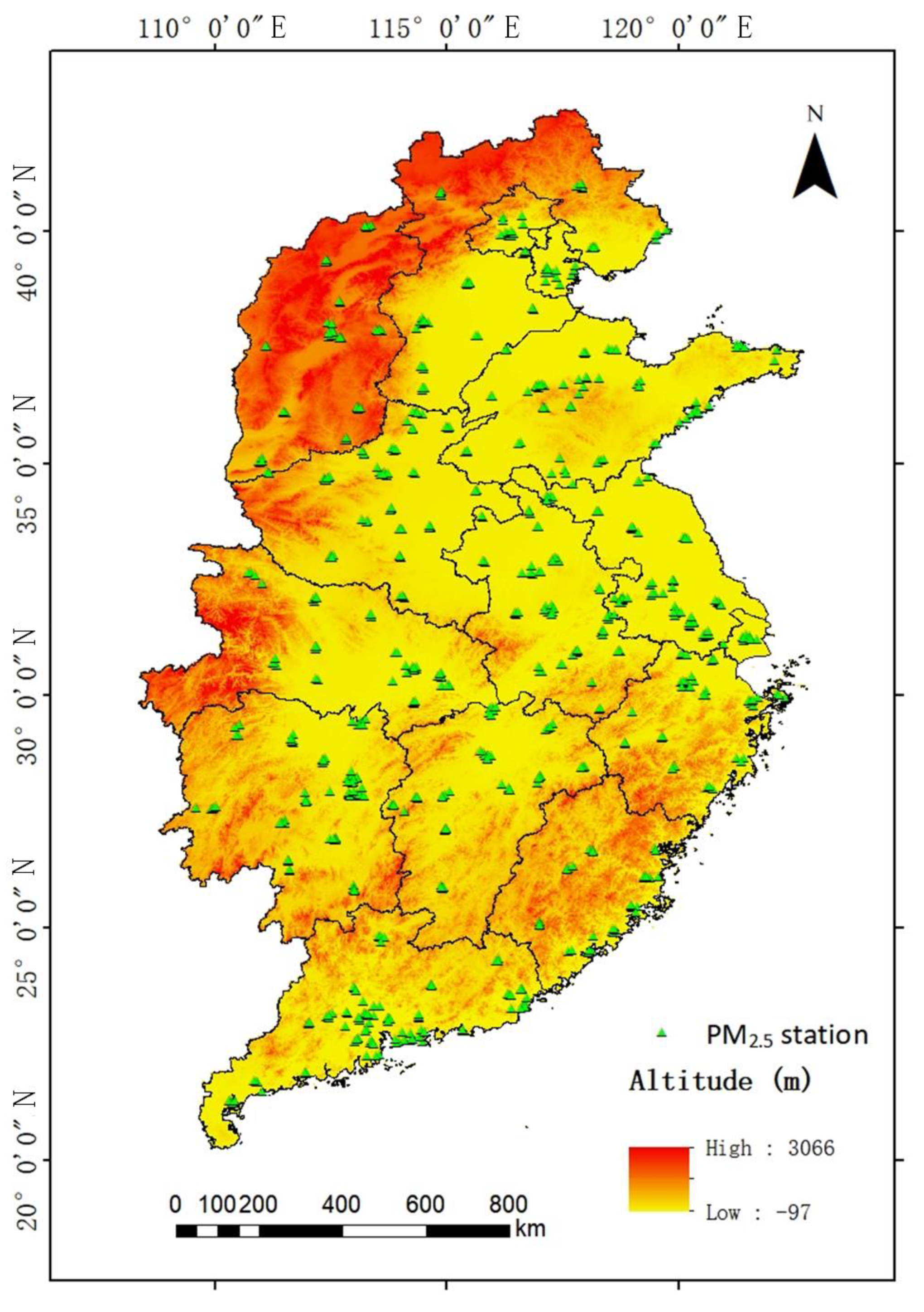
2.1. Study Area
2.2. Data Sources
2.2.1. PM2.5 Ground Measurements
2.2.2. MODIS AOD Products
2.2.3. Auxiliary Data
2.3. Methodology
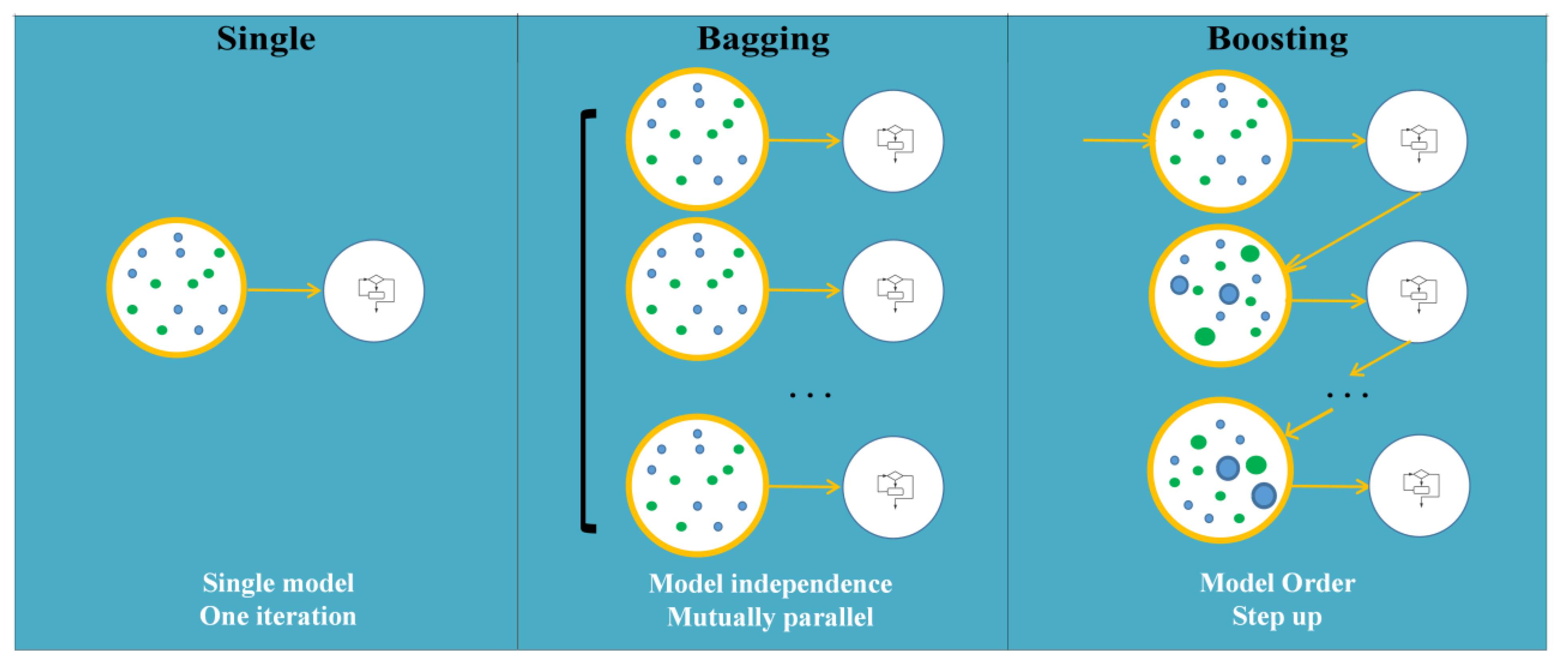
2.3.1. Machine-Learning (ML) Models
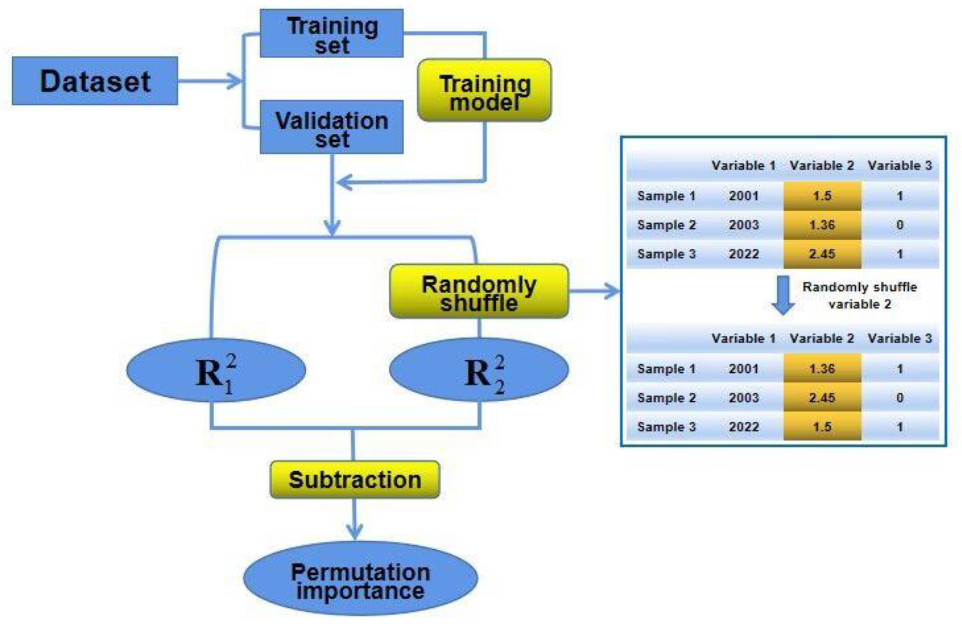
2.3.2. Importance Assessment Method
2.3.3. Model Validation Methods
2.3.4. Sensitivity Analysis Methods
- (1)
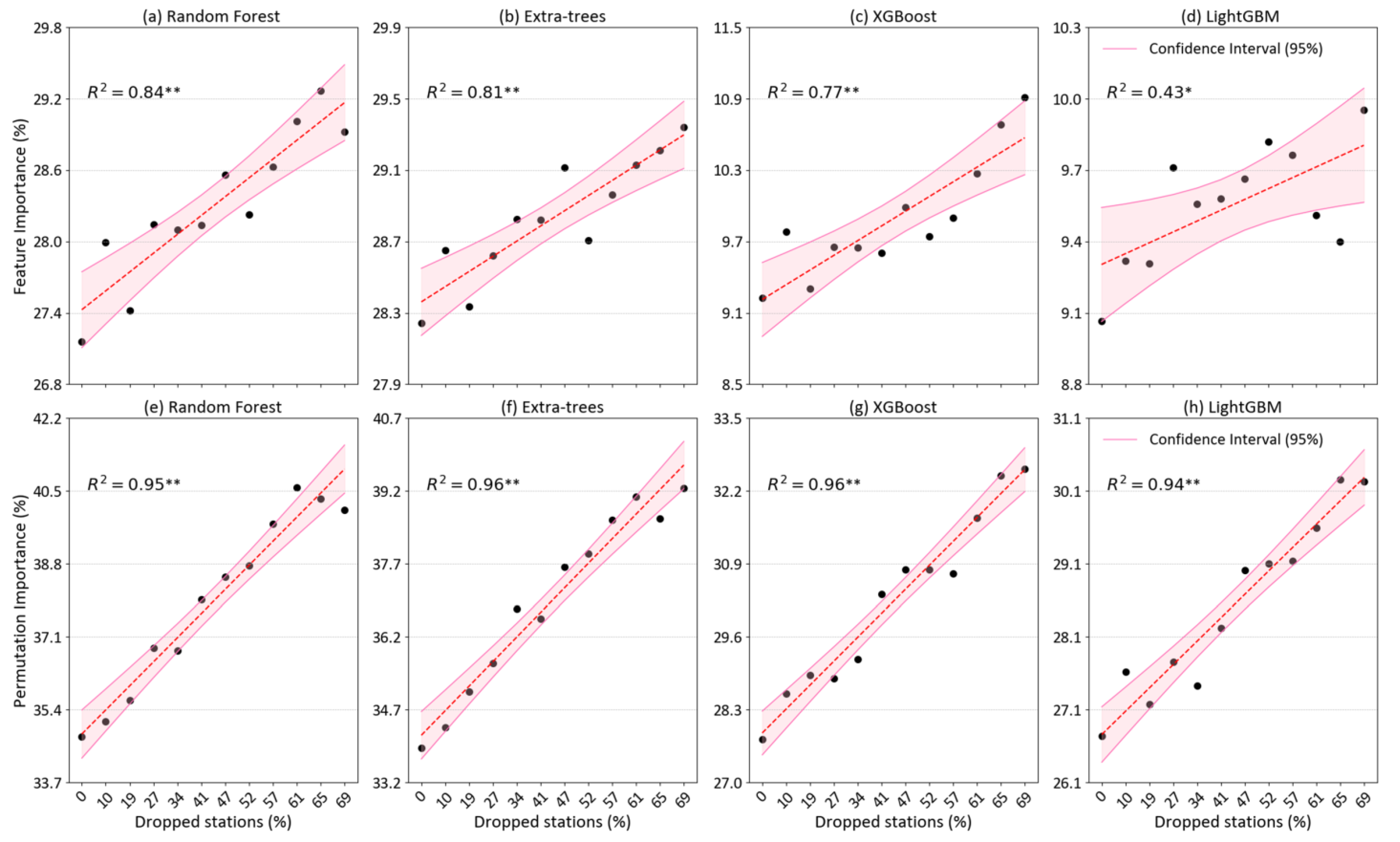
- The importance scores of satellite AOD were first calculated employing two techniques (FI and PI) for four typical tree-based ML models as the density of ground-based stations in the study area gradually decreased. This analysis offers valuable insights into the role of satellite AOD in the modeling process. It allows for an understanding of the significance of satellite AOD under different station-density conditions.
- (2)
- The accuracies and differences in the estimation of PM2.5, with and without satellite AOD as the primary predictor, were calculated using the sample-based 10-CV method. Four typical tree-based ML models were employed, each taking into consideration the decreasing density of ground-based stations in the study area. This analysis allows us to evaluate the importance of satellite AOD in enhancing the overall accuracy of PM2.5 estimates for varying station densities.
- (3)
- Similarly, the accuracies and differences in the prediction of PM2.5 in regions lacking PM2.5 observations, with and without satellite AOD as the main predictor, were calculated using the station-based 10-CV method. Again, four typical tree-based ML models were employed, each taking into consideration the decreasing density of ground-based stations in the study area. This analysis enables us to assess the significance of satellite AOD in improving the predictive ability of PM2.5 predictions for varying station densities.
3. Results
3.1. Variations of Satellite AOD Contributions
3.2. Impacts of Satellite AOD on Overall Accuracy
3.3. Impacts of Satellite AOD on Predictive Ability
4. Conclusions
Author Contributions
Funding
Data Availability Statement
Acknowledgments
Conflicts of Interest
References
- IPCC 2021. Climate Change, 2021: The Physical Science Basis; Contribution of Working Group I to the Fifth Assessment Report of the Intergovernmental Panel on Climate Change IPCC Working Group I Contribution to AR5Rep.; Cambridge University Press: Cambridge, UK; New York, NY, USA, 2021. [Google Scholar]
- Guo, J.; Xia, F.; Zhang, Y.; Liu, H.; Li, J.; Lou, M.; He, J.; Yan, Y.; Wang, F.; Min, M.; et al. Impact of diurnal variability and meteorological factors on the PM2.5-AOD relationship: Implications for PM2.5 remote sensing. Environ. Poll. 2017, 221, 94. [Google Scholar] [CrossRef] [PubMed] [Green Version]
- Li, Z.; Wang, Y.; Guo, J.; Zhao, C.; Cribb, M.C.; Dong, X.; Fan, J.; Gong, D.; Huang, J.; Jiang, M.; et al. East Asian Study of Tropospheric Aerosols and their Impact on Regional Clouds, Precipitation, and Climate (EAST-AIRCPC). J. Geophys. Res. Atmos. 2019, 124, 13026–13054. [Google Scholar] [CrossRef] [Green Version]
- Duyzer, J.; van den Hout, D.; Zandveld, P.; van Ratingen, S. Representativeness of air quality monitoring networks. Atmos. Environ. 2015, 104, 88–101. [Google Scholar] [CrossRef]
- Alsahli, M.M.; Al-Harbi, M. Allocating optimum sites for air quality monitoring stations using GIS suitability analysis. Urban Clim. 2018, 24, 875–886. [Google Scholar] [CrossRef]
- Chen, N.; Yang, M.; Du, W.; Min, H. PM2.5 estimation and spatial-temporal pattern analysis based on the modified support vector regression model and the 1 km resolution MAIAC AOD in Hubei, China. ISPRS Int. J. Geo-Inf. 2021, 10, 31. [Google Scholar] [CrossRef]
- van Donkelaar, A.; Martin, R.V.; Park, R.J. Estimating ground-level PM2.5 using aerosol optical depth determined from satellite remote sensing. J. Geophys. Res. Atmos. 2006, 111, D21201. [Google Scholar] [CrossRef]
- Ma, X.; Wang, J.; Yu, F.; Jia, H.; Hu, Y. Can MODIS AOD be employed to derive PM2.5 in Beijing-Tianjin-Hebei over China? Atmos. Res. 2016, 181, 250–256. [Google Scholar] [CrossRef]
- Li, S.; Joseph, E.; Min, Q. Remote sensing of ground-level PM2.5 combining AOD and backscattering profile. Remote Sens. Environ. 2016, 183, 120–128. [Google Scholar] [CrossRef]
- Li, Z.; Goloub, P.; Devaux, C.; Gu, X.; Qiao, Y.; Zhao, F.; Chen, H. Aerosol polarized phase function and single-scattering albedo retrieved from ground-based measurements. Atmos. Res. 2004, 71, 233–241. [Google Scholar] [CrossRef]
- Gupta, P.; Christopher, S.A.; Wang, J.; Gehrig, R.; Lee, Y.; Kumar, N. Satellite remote sensing of particulate matter and air quality assessment over global cities. Atmos. Environ. 2006, 40, 5880–5892. [Google Scholar] [CrossRef]
- Kumar, N. What can affect AOD–PM2.5 association? Environ. Health Perspect. 2010, 118, A109–A110. [Google Scholar] [CrossRef] [PubMed] [Green Version]
- Wang, J.; Christopher, S.A. Intercomparison between satellite-derived aerosol optical thickness and PM2.5 mass: Implications for air quality studies. Geophys. Res. Lett. 2003, 30, 2095. [Google Scholar] [CrossRef]
- Natunen, A.; Arola, A.; Mielonen, T.; Huttunen, J.; Lehtinen, K.E.J. A multi-year comparison of PM2.5 and AOD for the Helsinki region. Boreal Environ. Res. 2010, 15, 544–552. [Google Scholar] [CrossRef]
- Kloog, I.; Nordio, F.; Coull, B.A.; Schwartz, J. Incorporating local land use regression and satellite aerosol optical depth in a hybrid model of spatiotemporal PM2.5 exposures in the Mid-Atlantic states. Environ. Sci. Technol. 2012, 46, 11913–11921. [Google Scholar] [CrossRef] [PubMed] [Green Version]
- Ma, Z.; Hu, X.; Sayer, A.M.; Levy, R.; Zhang, Q.; Xue, Y.; Tong, S.; Bi, J.; Huang, L.; Liu, Y. Satellite-based spatiotem-poral trends in PM2. 5 concentrations: China 2004-2013. Environ. Health Perspect. 2016, 124, 184–192. [Google Scholar] [CrossRef] [Green Version]
- Qu, W.; Wang, J.; Zhang, X.; Sheng, L.; Wang, W. Opposite seasonality of the aerosol optical depth and the surface particulate matter concentration over the North China Plain. Atmos. Environ. 2016, 127, 90–99. [Google Scholar] [CrossRef]
- Su, T.; Li, Z.; Kahn, R. Relationships between the planetary boundary layer height and surface pollutants derived from lidar observations over China: Regional pattern and influencing factors. Atmos. Chem. Phys. 2018, 18, 15921–15935. [Google Scholar] [CrossRef] [Green Version]
- Koelemeijer, R.B.A.; Homan, C.D.; Matthijsen, J. Comparison of spatial and temporal variations of aerosol optical thickness and particulate matter over Europe. Atmos. Environ. 2006, 40, 5304–5315. [Google Scholar] [CrossRef]
- Brauer, M.; Amann, M.; Burnett, R.T.; Cohen, A.; Dentener, F.; Ezzati, M.; Henderson, S.B.; Krzyzanowski, M.; Martin, R.V.; Van Dingenen, R.; et al. Exposure assessment for estimation of the global burden of disease attributable to outdoor air pollution. Environ. Sci. Technol. 2012, 46, 652–660. [Google Scholar] [CrossRef] [Green Version]
- Chen, J.; de Hoogh, K.; Gulliver, J.; Hoffmann, B.; Hertel, O.; Ketzel, M.; Bauwelinck, M.; van Donkelaar, A.; Hvidtfeldt, U.A.; Katsouyanni, K.; et al. A comparison of linear regression, regularization, and machine learning algorithms to develop Europe-wide spatial models of fine particles and nitrogen dioxide. Environ. Int. 2019, 130, 104934. [Google Scholar] [CrossRef]
- Gupta, P.; Christopher, S. Particulate matter air quality assessment using integrated surface, satellite, and meteorological products: Multiple regression approach. J. Geophys. Res. Atmos. 2009, 114, D14205. [Google Scholar] [CrossRef] [Green Version]
- Ma, Z.; Hu, X.; Huang, L.; Bi, J.; Liu, Y. Estimating ground-level PM2.5 in China using satellite remote sensing. Environ. Sci. Tech. 2014, 48, 7436–7444. [Google Scholar] [CrossRef] [PubMed]
- You, W.; Zang, Z.; Zhang, L.; Li, Y.; Wang, W. Estimating national-scale ground-level PM2.5 concentration in China using geographically weighted regression based on MODIS and MISR AOD. Environ. Sci. Pollut. Res. 2016, 23, 8327–8338. [Google Scholar] [CrossRef]
- He, Q.; Huang, B. Satellite-based mapping of daily high-resolution ground PM2.5 in China via space-time regression modeling. Remote Sens. Environ. 2018, 206, 72–83. [Google Scholar] [CrossRef]
- Xiao, Q.; Wang, Y.; Chang, H.H.; Meng, X.; Liu, Y. Full-coverage high-resolution daily PM2.5 estimation using MAIAC AOD in the Yangtze River Delta of China. Remote Sens. Environ. 2017, 199, 437–446. [Google Scholar] [CrossRef]
- Liu, Y.; Sarnat, J.A.; Kilaru, A.; Jacob, D.J.; Koutrakis, P. Estimating ground-level PM2.5 in the eastern United States using satellite remote sensing. Environ. Sci. Technol. 2005, 39, 3269–3278. [Google Scholar] [CrossRef] [Green Version]
- Lee, H.J.; Liu, Y.; Coull, B.A.; Schwartz, J.; Koutrakis, P. A novel calibration approach of MODIS AOD data to predict PM2.5 concentrations. Atmos. Chem. Phys. 2011, 11, 7991–8002. [Google Scholar] [CrossRef] [Green Version]
- Chen, W.; Ran, H.; Cao, X.; Wang, J.; Zheng, X. Estimating PM2.5 with high-resolution 1-km AOD data and an improved machine learning model over Shenzhen, China. Sci. Total Environ. 2020, 746, 141093. [Google Scholar] [CrossRef]
- Wei, J.; Huang, W.; Li, Z.; Xue, W.; Cribb, M. Estimating 1-km-resolution PM2.5 concentrations across China using the space-time random forest approach. Remote Sens. Environ. 2019, 231, 111221. [Google Scholar] [CrossRef]
- Wei, J.; Li, Z.; Cribb, M.; Huang, W.; Xue, W.; Sun, L.; Guo, J.; Peng, Y.; Li, J.; Lyapustin, A.; et al. Improved 1-km-resolution PM2.5 estimates across China using enhanced space-time extremely randomized trees. Atmos. Chem. Phys. 2020, 20, 3273–3289. [Google Scholar] [CrossRef] [Green Version]
- Wei, J.; Li, Z.; Lyapustin, A.; Sun, L.; Peng, Y.; Xue, W.; Su, T.; Cribb, M. Reconstructing 1-km-resolution high-quality PM2.5 data records from 2000 to 2018 in China: Spatiotemporal variations and policy implications. Remote Sens. Environ. 2021, 252, 112136. [Google Scholar] [CrossRef]
- Pan, B. Application of XGBoost algorithm in hourly PM2.5 concentration prediction. IOP Conf. Ser. Earth Environ. Sci. 2018, 113, 012127. [Google Scholar] [CrossRef] [Green Version]
- Wei, J.; Li, Z.; Pinker, R.T.; Sun, L.; Li, R. Himawari-8-derived diurnal variations of ground-level PM2.5 pollution across China using the fast space-time Light Gradient Boosting Machine (LightGBM). Atmos. Chem. Phys. 2021, 21, 7863–7880. [Google Scholar] [CrossRef]
- Fang, X.; Zou, B.; Liu, X.; Sternberg, T.; Zhai, L. Satellite-based ground PM2.5 estimation using timely structure adaptive modeling. Remote Sens. Environ. 2016, 186, 152–163. [Google Scholar] [CrossRef]
- Meng, X.; Fu, Q.; Ma, Z.; Chen, L.; Zou, B.; Zhang, Y.; Xue, W.; Wang, J.; Wang, D.; Han, H. Estimating ground-level PM10 in a Chinese city by combining satellite data, meteorological information and a land use regression model. Environ. Pollut. 2016, 208, 177–184. [Google Scholar] [CrossRef] [PubMed]
- Pereira, G.; Lee, H.J.; Bell, M.; Regan, A.; Malacova, E.; Mullins, B.; Knibbs, L.D. Development of a model for particulate matter pollution in Australia with implications for other satellite-based models. Environ. Res. 2017, 159, 9–15. [Google Scholar] [CrossRef] [PubMed] [Green Version]
- Chen, G.; Li, Y.; Zhou, Y.; Shi, C.; Liu, Y. The comparison of AOD-based and non-AOD prediction models for daily PM2.5 estimation in Guangdong province, China with poor AOD coverage. Environ. Res. 2021, 195, 110735. [Google Scholar] [CrossRef] [PubMed]
- Yu, W.; Li, S.; Ye, T.; Xu, R.; Song, J.; Guo, Y. Deep ensemble machine learning framework for the estimation of PM2.5 concentrations. Environ. Health Perspect. 2022, 130, 037004. [Google Scholar] [CrossRef]
- Lyapustin, A.; Martonchik, J.; Wang, Y.; Laszlo, I.; Korkin, S. Multi-Angle Implementation of Atmospheric Correction (MAIAC): 1. Radiative transfer basis and look-up tables. J. Geophys. Res. Atmos. 2011, 116, D03210. [Google Scholar] [CrossRef]
- Lyapustin, A.; Wang, Y.; Korkin, S.; Huang, D. MODIS Collection 6 MAIAC algorithm. Atmos. Meas. Tech. 2018, 11, 5741–5765. [Google Scholar] [CrossRef] [Green Version]
- Hersbach, H.; Bell, B.; Berrisford, P.; Hirahara, S.; Horányi, A.; Muñoz-Sabater, J.; Nicolas, J.; Peubey, C.; Radu, R.; Schepers, D.; et al. The ERA5 global reanalysis. Q. J. R. Meteorol. Soc. 2020, 146, 1999–2049. [Google Scholar] [CrossRef]
- Peuch, V.H.; Engelen, R.; Ades, M.; Barre, J.; Suttie, M. The use of satellite data in the Copernicus Atmosphere Monitoring Service (CAMS). In IGARSS 2018–2018 IEEE International Geoscience and Remote Sensing Symposium; IEEE: Manhattan, NY, USA, 2018. [Google Scholar]
- Wei, J.; Li, Z.; Wang, J.; Li, C.; Gupta, P.; Cribb, M. Ground-level gaseous pollutants (NO2, SO2, and CO) in China: Daily seamless mapping and spatiotemporal variations. Atmos. Chem. Phys. 2023, 23, 1511–1532. [Google Scholar] [CrossRef]
- Malakar, N.K.; Lary, D.J.; Moore, A.; Gencaga, D.; Roscoe, B.; Albayrak, A.; Petrenko, M.; Wei, J. Estimation and bias correction of aerosol abundance using data-driven machine learning and remote sensing. In Proceedings of the 2012 Conference on Intelligent Data Understanding (CIDU 2012), Boulder, CO, USA, 24–26 October 2012. [Google Scholar]
- Lary, D.J.; Faruque, F.S.; Malakar, N.; Moore, A.; Roscoe, B.; Adams, Z.L.; Eggelston, Y. Estimating the global abundance of ground level presence of particulate matter (PM2.5). Geospat. Health 2014, 8, S611–S630. [Google Scholar] [CrossRef] [Green Version]
- Reid, C.E.; Jerrett, M.; Petersen, M.L.; Pfister, G.G.; Morefield, P.E.; Tager, I.B.; Raffuse, S.M.; Balmes, J.R. Spatiotemporal prediction of fine particulate matter during the 2008 northern California wildfires using machine learning. Environ. Sci. Technol. 2015, 49, 3887–3896. [Google Scholar] [CrossRef] [PubMed]
- Breiman, L. Random forests. Mach. Learn. 2002, 45, 5–32. [Google Scholar] [CrossRef] [Green Version]
- Chen, G.; Li, S.; Knibbs, L.D.; Hamm, N.A.S.; Cao, W.; Li, T.; Guo, J.; Ren, H.; Abramson, M.J.; Guo, Y. A machine learning method to estimate PM2.5 concentrations across China with remote sensing, meteorological and land use information. Sci. Total Environ. 2018, 636, 52–60. [Google Scholar] [CrossRef]
- Hu, X.; Belle, J.H.; Meng, X.; Wildani, A.; Waller, L.A.; Strickland, M.J.; Liu, Y. Estimating PM2.5 concentrations in the conterminous United States using the random forest approach. Environ. Sci. Tech. 2017, 51, 6936–6944. [Google Scholar] [CrossRef]
- Geurts, P.; Ernst, D.; Wehenkel, L. Extremely randomized trees. Mach. Learn. 2006, 63, 3–42. [Google Scholar] [CrossRef] [Green Version]
- Chen, T.; Guestrin, C. XGBoost: A scalable tree boosting system. In Proceedings of the 22nd ACM SIGKDD International Conference on Knowledge Discovery and Data Mining, San Francisco, CA, USA, 13–17 August 2016; pp. 785–794. [Google Scholar]
- Ke, G.; Meng, Q.; Finley, T.; Wang, T.; Chen, W.; Ma, W.; Ye, Q.; Liu, T. LightGBM: A highly effificient gradient boosting decision tree. In Advances in Neural Information Processing Systems; ACM: Long Beach, CA, USA, 2017; pp. 3149–3157. Available online: https://dl.acm.org/doi/10.5555/3294996.3295074 (accessed on 1 January 2020).
- Loecher, M. Unbiased variable importance for random forests. Commun. Stat. Theory Methods 2022, 51, 1413–1425. [Google Scholar] [CrossRef]
- Kim, H.; Loh, W.-Y. Classification trees with unbiased multiway splits. J. Am. Stat. Assoc. 2001, 96, 589–604. [Google Scholar] [CrossRef] [Green Version]
- Rodriguez, J.; Perez, A.; Lozano, J. Sensitivity analysis of k-fold cross validation in prediction error estimation. IEEE Trans. Pattern Anal. Mach. Intell. 2010, 32, 569–575. [Google Scholar] [CrossRef] [PubMed]
- Wei, J.; Li, Z.; Chen, X.; Li, C.; Sun, Y.; Wang, J.; Lyapustin, A.; Brasseur, G.; Jiang, M.; Sun, L.; et al. Separating daily 1-km PM2.5 inorganic chemical composition in China since 2000 via deep learning integrating ground, satellite, and model data. Environ. Sci. Tech. 2023. [Google Scholar] [CrossRef] [PubMed]
- Wei, J.; Li, Z.; Xue, W.; Sun, L.; Fan, T.; Liu, L.; Su, T.; Cribb, M. The ChinaHighPM10 dataset: Generation, validation, and spatiotemporal variations from 2015 to 2019 across China. Environ. Int. 2021, 146, 106290. [Google Scholar] [CrossRef] [PubMed]
- Wei, J.; Liu, S.; Li, Z.; Liu, C.; Qin, K.; Liu, X.; Pinker, R.; Dickerson, R.; Lin, J.; Boersma, K.; et al. Ground-level NO2 surveillance from space across China for high resolution using interpretable spatiotemporally weighted artificial intelligence. Environ. Sci. Tech. 2022, 56, 9988–9998. [Google Scholar] [CrossRef] [PubMed]


Disclaimer/Publisher’s Note: The statements, opinions and data contained in all publications are solely those of the individual author(s) and contributor(s) and not of MDPI and/or the editor(s). MDPI and/or the editor(s) disclaim responsibility for any injury to people or property resulting from any ideas, methods, instructions or products referred to in the content. |
© 2023 by the authors. Licensee MDPI, Basel, Switzerland. This article is an open access article distributed under the terms and conditions of the Creative Commons Attribution (CC BY) license (https://creativecommons.org/licenses/by/4.0/).
Share and Cite
Tian, Z.; Wei, J.; Li, Z. How Important Is Satellite-Retrieved Aerosol Optical Depth in Deriving Surface PM2.5 Using Machine Learning? Remote Sens. 2023, 15, 3780. https://doi.org/10.3390/rs15153780
Tian Z, Wei J, Li Z. How Important Is Satellite-Retrieved Aerosol Optical Depth in Deriving Surface PM2.5 Using Machine Learning? Remote Sensing. 2023; 15(15):3780. https://doi.org/10.3390/rs15153780
Chicago/Turabian StyleTian, Zhongyan, Jing Wei, and Zhanqing Li. 2023. "How Important Is Satellite-Retrieved Aerosol Optical Depth in Deriving Surface PM2.5 Using Machine Learning?" Remote Sensing 15, no. 15: 3780. https://doi.org/10.3390/rs15153780