1. Introduction
In the inverse electromagnetic scattering problem, the goal is to determine the permittivity and permeability of an unknown scatterer and identify its shape and location. This is achieved by using information about the scattered field, obtained through the illumination of the scatterer with a known incident field. This problem is of great interest because of its applications in various areas of physics and engineering; for instance, radar imaging [
1], synthetic-aperture radar (SAR) imaging [
2,
3], remote sensing [
4,
5], ground penetrating radar (GPR) [
6,
7], civil engineering applications of GPR [
8], geophysics application of GPR [
9], and medical imaging [
10,
11,
12]. The near or far field can be considered in terms of the favorite application.
When considering objects with significant differences in dielectric properties, such as strong contrasts, or objects that are very large in terms of the wavelength, multiple scattering becomes a significant factor to take into account. Therefore, the problem becomes strongly non-linear and requires the use of iterative approaches for its solution. Then, solution algorithms are based on the minimization of an error function. Stochastic methods are applicable when the number of unknowns is very low due to their heavy computational burden. On the other hand, iterative and gradient based approaches may converge to false solutions, according to the choice of the starting point. Therefore, all these methods do not allow consideration of the mathematical features of the operator to be inverted so as to predict their ultimate results. On the contrary, linear approximations allow investigation of their results and their limitations. To this end, it is common to consider the pertinent so-called point spread function (PSF) in tomographic approaches in order to appreciate the resolution of the algorithm. In this paper, we attempt to find a closed form expression for the PSF in the case of single frequency excitation and to validate it numerically.
Linear scattering models also arise in iterative non-linear method such as the Born iterative method (BIM) [
13] and the distorted Born iterative (DBI) [
14,
15]. Therefore, an accurate analysis of the linear inverse scattering problem deserves attention in order to understand the best expected performances in connection with the source and receiver locations. Hereafter, we consider the Born approximation.
We need to introduce two mathematical tools for our analysis. When the operator is linear and compact, the singular value decomposition (SVD) of the relevant operator can be applied to introduce the number of degrees of freedom (NDF) and PSF. For the operators of which we are interested in this paper, the compact operators whose singular values exponentially decay to 0, when the singular values exhibit a step-like behavior, NDF can then be estimated as the number of significant singular values before the knee or exponential decay. This number can be assumed as an estimate of the maximum achievable resolution, meaning the number of independent point-like scatterers that can be accurately reconstructed. However, determining the NDF in closed form is often a difficult task, except for specific geometries like linear, circumference, and circular geometries. For all other cases, one can attempt to derive an estimate or upper bound for the NDF through numerical means.
The NDF evaluation of scattered fields was addressed in [
16] for strip geometries, where it was found that the length of the strip matters in computing the NDF and the NDF of two linear scatterers can be computed by the matrix approach which is equal to the summation of the NDF of each strip when they are far apart. In [
17] it was shown that the NDF of a full 2D square source is equivalent to the NDF of a void square source, which is provided by summing the NDF of each side of the square. An analytical evaluation of the NDF of the radiated/scattered fields was provided in [
18] for circumference geometries and two concentric circumferences were considered to show that the NDF of two geometries is equal to the NDF of the outer circumference in the inverse source. Whereas in inverse scattering, the total NDF is the sum of each circumference.
The PSF represents the impulse response of the cascade formed by the operator and its regularized inverse. It provides the impulse response of a linear imaging system to a point-like object. Therefore, the width of its main lobe is related to the achievable resolution by the inversion process. This means that the response produced by any object can be represented as the convolution of the response due to a point-like scatterer with the spatial variation of the object itself. Using this method makes it possible to quickly and reliably reconstruct images of objects of good quality. The PSF is a fast and significant approach to computing the achievable image quality of the objects.
In addition, it is feasible to represent the regularized solution to the inverse problem using a truncated SVD (TSVD) by using an expansion in the right singular functions. Thus, in the reconstruction, the truncation index allows excluding from the reconstruction the components corresponding to small singular values, which eliminates the noise components. The behavior of the exact PSF is related to the truncation index that can be adapted in terms of the NDF, which means the unknown can be reconstructed reliably by an imaging algorithm, even when there are uncertainties present in the data. Nevertheless, the analytical form of the PSF is not always available when using TSVD inversion, and its determination may require a numerical approach.
The PSF concept was used in [
19] to perform holographic imaging of dielectric media. In [
20], the imaging resolutions of the time-reversal and back-projection algorithms were compared by analyzing their PSFs with numerical studies, and it was shown that both algorithms had the same imaging resolutions, whether in the free space or the layered media.
Earlier research in [
21] presented an approximate evaluation of the resolution for strip source/scattering geometries, assuming full data availability. The evaluation demonstrates that the approximation can effectively predict the resolution. Furthermore, the resolution is spatially invariant in the full-view case. The same analysis is available in [
18] for circumference source/scattering geometries. For the limited view case, a good approximation of the resolution was evaluated in [
22] for curve geometries and in [
23] for the full 2D geometries, and the studies found that a spatially variant of the resolution was achieved.
This paper addresses the evaluation of the PSF of the scattered field to estimate the achievable resolution for a single frequency and multi-view in the homogeneous medium in the near zone. In fact, there is no analytical evaluation of the exact PSF, and it should be determined numerically. To overcome these limitations, we propose an analytical approximation of the exact PSF. Our analysis covers two cases: the full-view case, where the incident field and observation ranges cover full angles, and the aspect-limited case, where the incident field and observation ranges are limited to a certain range of angles. In this analysis, we adopt a circumference geometry for the sensing system. While the analytical estimation of the NDF is known in [
23,
24] for the far field, we extend this approach to compute the NDF in the near field. We discuss how the NDF in both far and near fields is equal by providing a comparison between them for each case. Numerical simulations are provided for each case to confirm the analytical discussions. Finally, we show how to use analytical discussions for a localization application.
In this paper, we focus on the linear approximation of the scattering equations for dielectric objects in free space, specifically the Born approximation. However, the entire approach and the results can also be extended to other linear approximations of scattering. For instance, for a perfectly electric conducting object, the physical optics (PO) approximation [
25], arising from the radiation of equivalent approximate currents in free space, provides a linear approximation of the scattering operator very similar to the one considered hereafter. The PO approximation has been also extended to the scattering of a strong dielectric object so that it can be also invoked in the remote sensing of the Earth’s surface. In addition, we consider near field conditions, which are common in subsurface prospection by ground penetrating radars. Finally, the observation and the excitation domains are assumed to lay on an arc of the circumference, as it allows a closed form evaluation of some of the functions relevant in the chosen approach. However, in the aspect-limited case, a chord and circumference can approximate the arc. Therefore, the results can be expected to hold approximately for linear domains as well.
The following is the structure of the paper. In
Section 2, the problem statement and the approximate evaluation of the resolution for a general scattering geometry are presented.
Section 3 provides various numerical examples to support the theoretical discussions.
Section 4 provides a numerical application of the theoretical discussions. Finally, in
Section 5, conclusions and discussions are provided.
2. Statement of the Problem
In this section, we first provide some mathematical preliminaries and notations used in the following sections. Second, we recall the definition of the exact PSF and provide the evaluation of the approximated PSF.
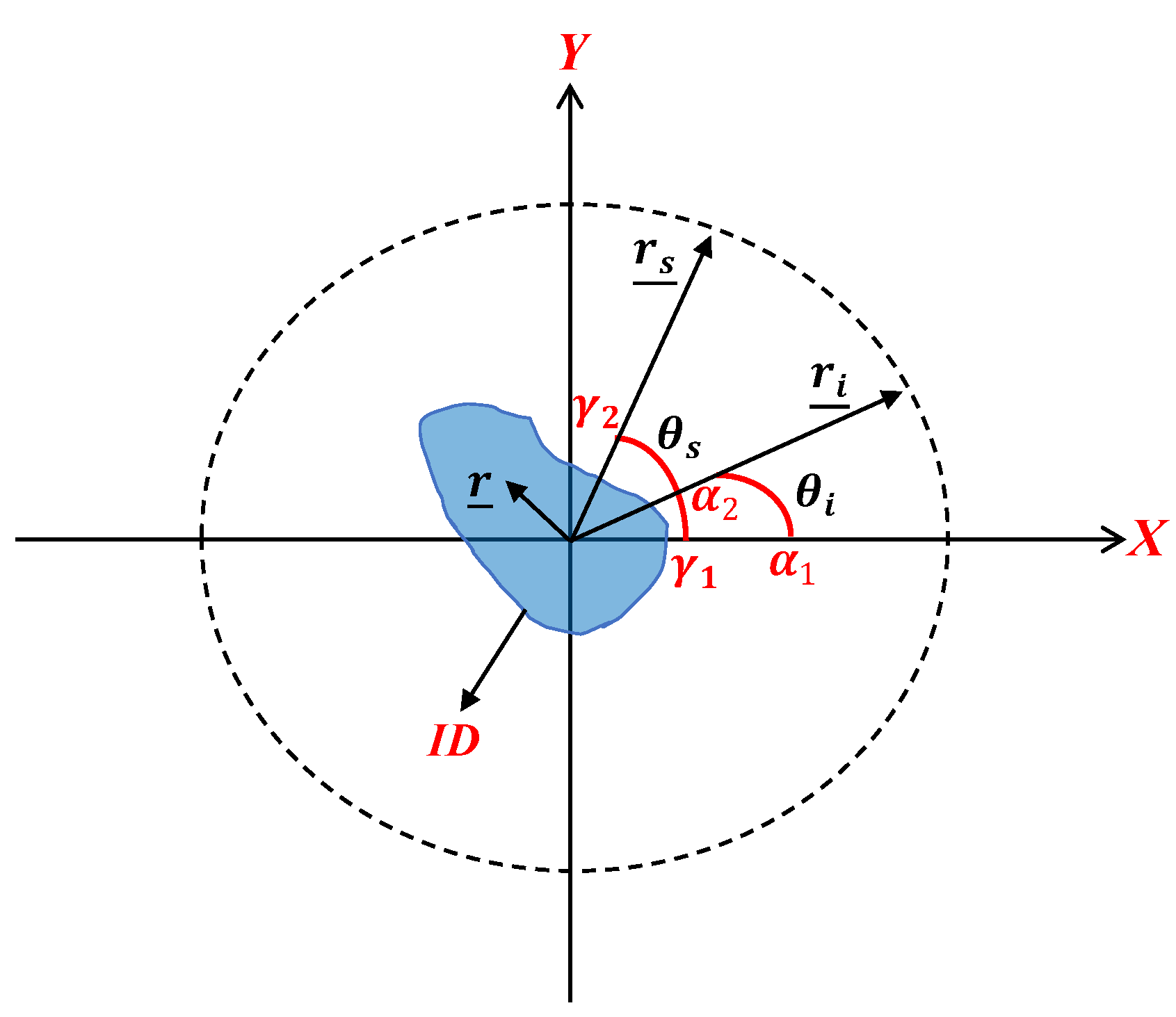
Figure 1 shows the general geometry of the problem in the near field. An unknown scatterer is located in a homogeneous domain referred to as the investigation domain (ID). The position vectors of the scattering object, the source point(transmitter), and the observation point (receiver) are denoted by
,
and
, respectively, where
and
are constant. The incident field and observations angular domains are supposed to be limited so that
and
.
The scattered field is defined by
where
is the Hankel function of the second kind and zero-th order.
and
are contrast function and pertinent linear operator for the multi-view and single frequency scattering configuration of our interest.
is equal to
, where
is the relative permittivity of the scatterer. We suppose that the scatterer is located in the free space as a homogenous background. Furthermore, the wavenumber and wavelength are indicated by
and
, respectively.
Approximate Evaluation of the Resolution
The achievable resolution in the inverse scattering problem may be impacted by factors such as the shape of the scattering geometry and the ranges of the incident field and observation domains. To assess the performance of the reconstruction algorithm and demonstrate its effectiveness in achieving resolution, the PSF concept is used. In this subsection, to provide a clear view of the mathematical details leading to the main analytical results of the paper, we present the individual steps as a numbered list.
The definition of the exact PSF. In the scatterer domain, the impulse response of an imaging system to a point-like scatterer is defined by the PSF concept and can be expressed by the cascade of the , i.e., the regularized inverse operator of and the direct operator. The PSF is observed at when the point-like scatterer is located at . In other words, the response of the system to a Dirac delta function is the PSF of the system. Mathematically, the exact PSF is defined by
Then, the SVD is applied to (1) because the
operator is linear and compact. Its singular system consists of
, where
and
are the singular functions, which span the data and the scatterer contrast function spaces, respectively, and
expresses the singular values by arranging them under a decreasing order [
26]. To define the TSVD inversion [
26], we can express (2) using the truncated completeness relation involving singular functions
. In this way, we can obtain the minimum-norm solution to the inverse scattering problem requiring the projection of the actual contrast function onto the singular function that possesses singular values that are not zero. Then, it can be shown as follows:
where the symbol (*) denotes the conjunction operation. Equation (3) expresses that the exact PSF depends on the number of retained singular values. The truncation index
is related to the accuracy of the solution and can be adopted in terms of the NDF.
- 2.
The introduction of the approximated PSF. To derive the closed-form expression of (3), it is necessary to have information about the singular functions, which cannot be calculated in closed form in general. However, according to [
18,
21,
22], the adjoint operator can approximate the inverse operator in (2) if the singular values of the relevant operator exhibit a nearly constant behavior before the knee of its curve. Therefore, if this condition is satisfied, we can substitute the inversion operator in (2) with the adjoint operator to build a good approximation of the PSF, which can overcome the aforementioned limitation. The goal is to provide an analytical evaluation of the approximated PSF to predict the resolution, while the approximated
is defined as follows:
- 3.
The analytical evaluation of (4). The adjoint operator of (1) is provided by
Then, the spectral theorem is applied to
, which is a compact self-adjoint operator.
whose kernel is as below:
- 4.
The addition theorem for the Hankel functions. This is invoked as a series representation as, for instance below:
where
is the Bessel function of the first kind and
n-th order and
is the Hankel function of the second kind and
n-th order.
By using (8) four times and interchanging the integrals with the summations, (7) becomes a four-fold summation, which can be factored as the product of two symmetrical functions with different arguments:
and are concerned with the observation and incident field, respectively.
- 5.
Residual closed form integration. The function can be written as a double summation:
whose terms
,
and
are as follows:
By performing the simple closed form integration in (11)b, the computation of
gives the following:
where
.
At the same time, the
function can be written as (10):
where
,
and
are now the following:
By performing the simple closed form integration in (14)b, the computation of
gives now the following:
- 6.
Final result. We can rewrite explicitly Equation (9) as below:
thus, providing the analytical expression of the approximated
. The summations can be safely truncated to
, as
is the maximum integer, due to asymptotic exponentially decay of the Bessel functions for indices larger than its argument, when
are smaller than
.
It should be noted that while the exact PSF depends on the truncation value of the TSVD algorithm, which depends on the NDF of the problem, the
is independent of it. Therefore, to assess the performance of the
, it is important to estimate the NDF pertinent to the scattering geometry and use this information to truncate the SVD. This will allow for a fair comparison between the approximate and exact PSFs. In the
Appendix A, a discussion is provided on how to estimate the NDF in the case of aspect limited data in the near field.
3. Numerical Validation
This section provides numerical examples to validate the analytical discussions and to demonstrate the effectiveness of the approximated PSF. Specifically, a circle ID with a radius of is considered. As far as the numerical inversion of the integral Equation (1) is concerned, in order to achieve a good approximation of the continuous operator, the simple choice of a sufficiently polar dense grid to achieve a step on both arc and radial variables is adopted. The SVD of the resulting matrix equation is computed in the MATLAB environment. In this way, we may obtain the exact PSF by truncating the SVD to the exact NDF.
In the following numerical examples, and are both equal to . Moreover, only the main lobe of the PSF is considered to highlight its focusing properties, and the amplitudes of both PSFs are normalized to 1.
In order to compute the NDF of the considered ID, we use the analytical result provided in [
23,
24] for the far scattered field concerning the evaluation of the NDF for the double Fourier transform operator. In fact, for far zone observation, the scattering operator (1) can be cast as such by an appropriate change of variables form the angular to the spectral ones. Then, a closed form value of the NDF is known in the literature and employed here: it requires only to know the measure
of the ID and
of the spectral domain area. In turn this depends on the ranges of excitation and observation angles. Therefore, the NDF for the far scattered field is provided by the following:
where
for the considered ID. More detailed information is available for computing
in [
23].
First, numerical examples are presented for the full-view case in
Section 3.1. Then, different examples are provided for the aspect-limited case in
Section 3.2.
3.1. Full-View Case
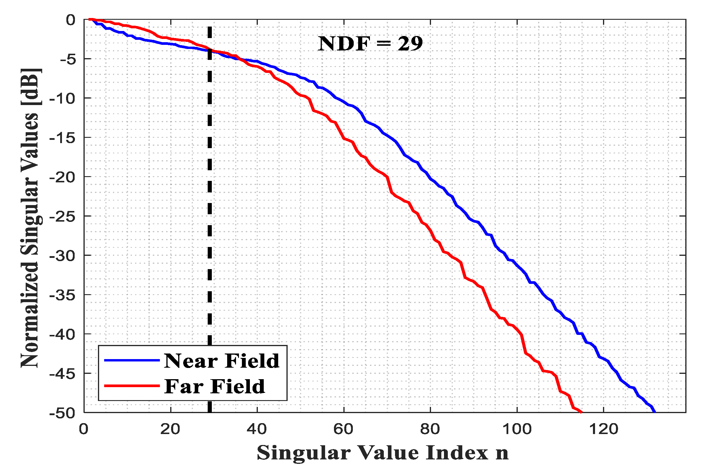
In this subsection, we consider the full view case where the angular ranges of the excitation and observation directions are wide. This means that and are equal to , whereas and are .
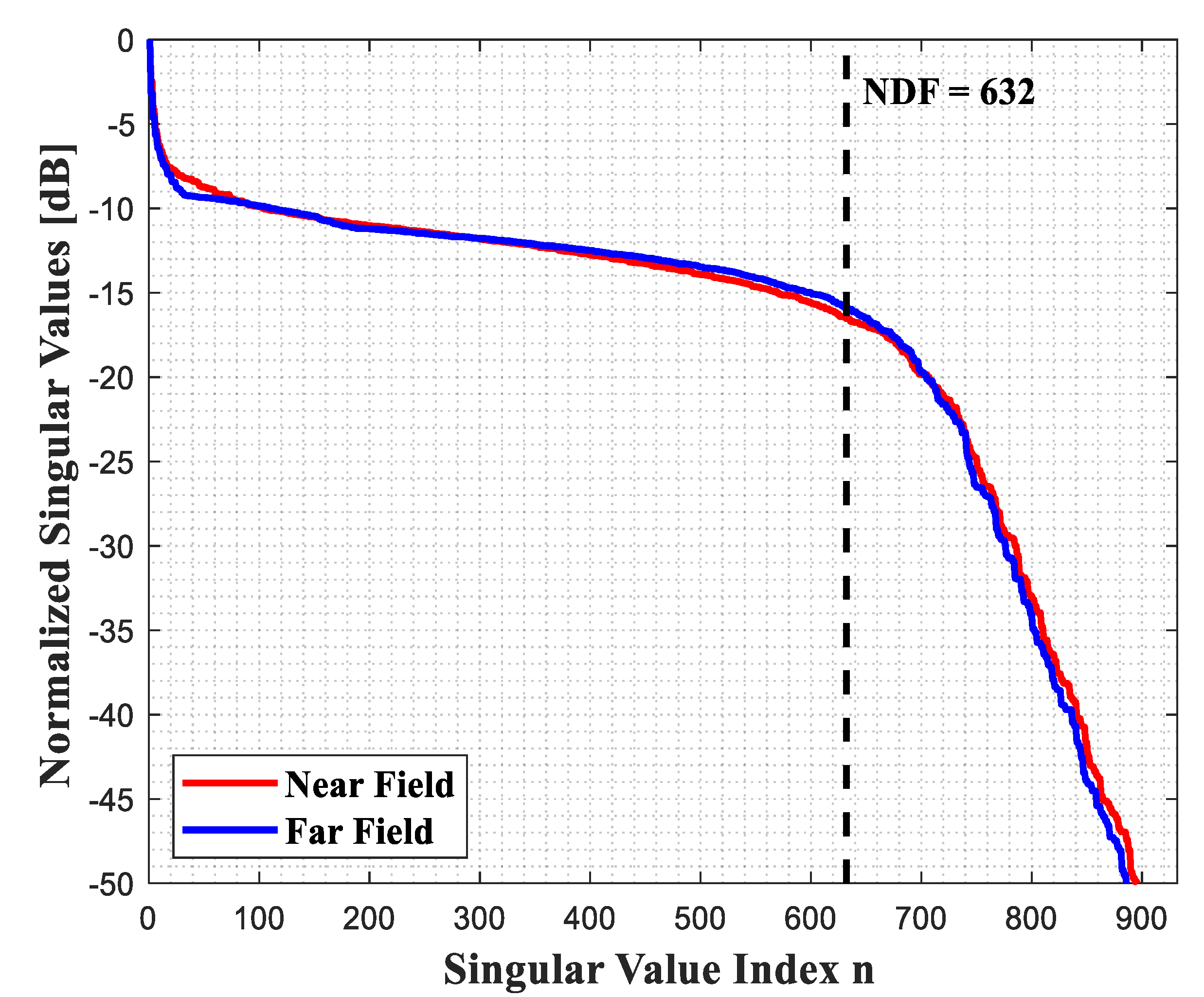
First, we compare the NDF of both the far and near scattered field and compute them numerically by referring to the pertinent far zone operator [
23,
24] and to (1), respectively.
Figure 2 provides a comparison of the behaviours of their normalized singular values. The expected NDF of the far field from (17) is equal to NDF =
, as
and the numerical results confirm that the NDF in the near field is equal to the NDF of the far field. This result can be expected in virtue of the equivalence theorem, as for each source the corresponding near scattered field has the same NDF of the corresponding far field.
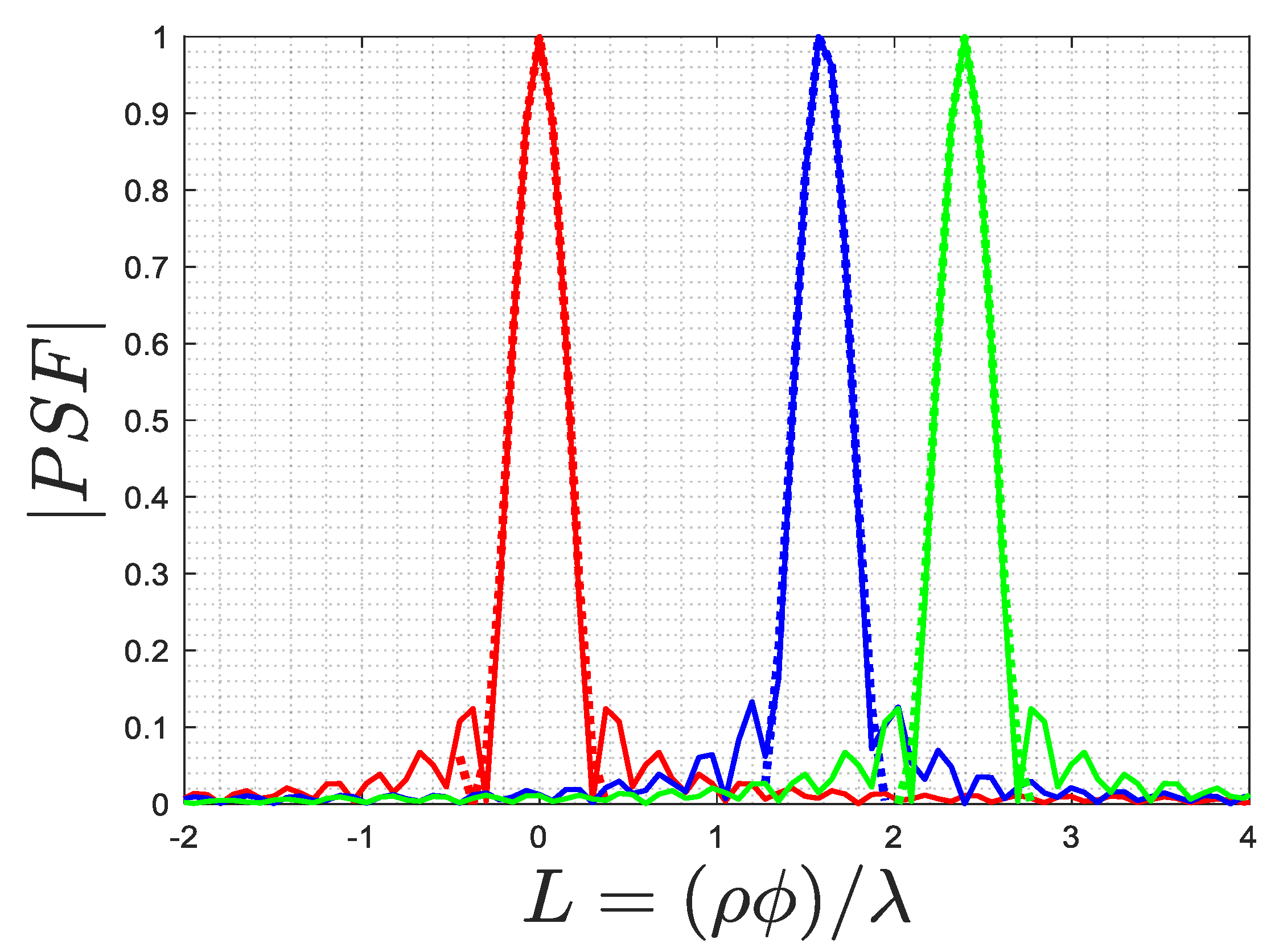
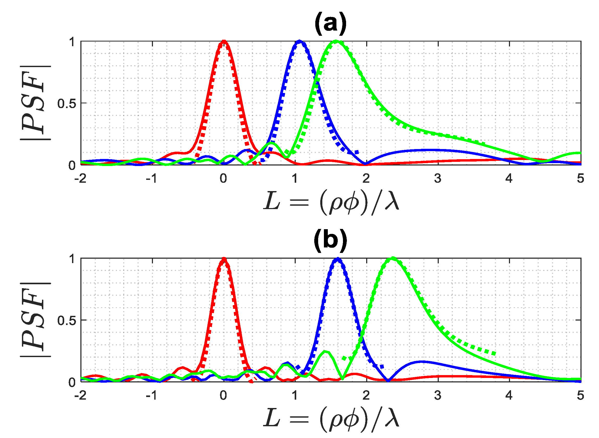
In order to assess the performance of the
in achieving the resolution, a comparison is made between the normalized amplitude of the exact and approximated PSFs cut along
in
Figure 3. The results are presented for three point-like scatterers when
. The findings demonstrate that the resolution remains space-invariant and confirm a significant overlap between the
and the exact PSF in the main lobes. This reliable prediction of the achievable resolution applies to every point-like scatterer.
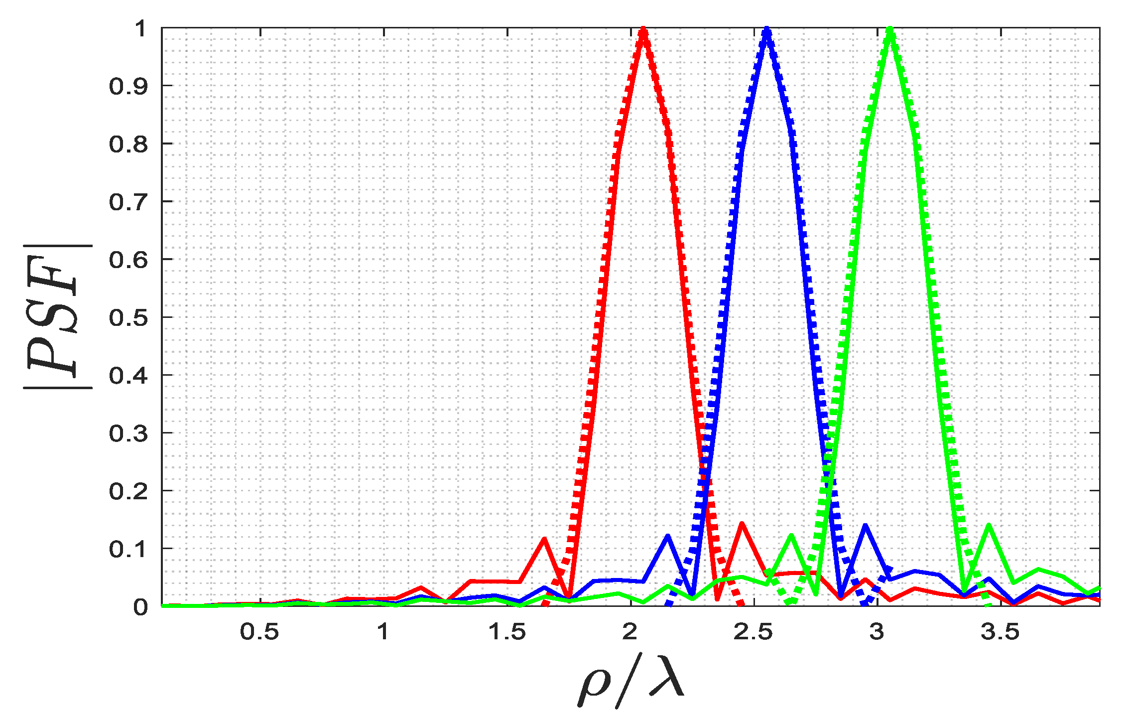
Next, we compare both PSFs for
-cut when
, as illustrated in
Figure 4. As observed, the space invariance is once again achieved and the approximated
also performs well.
3.2. Aspect-Limited Observation and Excitation
In this subsection, we consider the aspect limited case when the system is in reflection mode where the angular ranges of the excitation and observation directions are
wide. This means that
and
are equal to
, while
and
are
. The spectral domain area
is computed in [
23] for this angular range, which is
. Hence, the NDF of the far field can be analytically derived from (17), which is
.
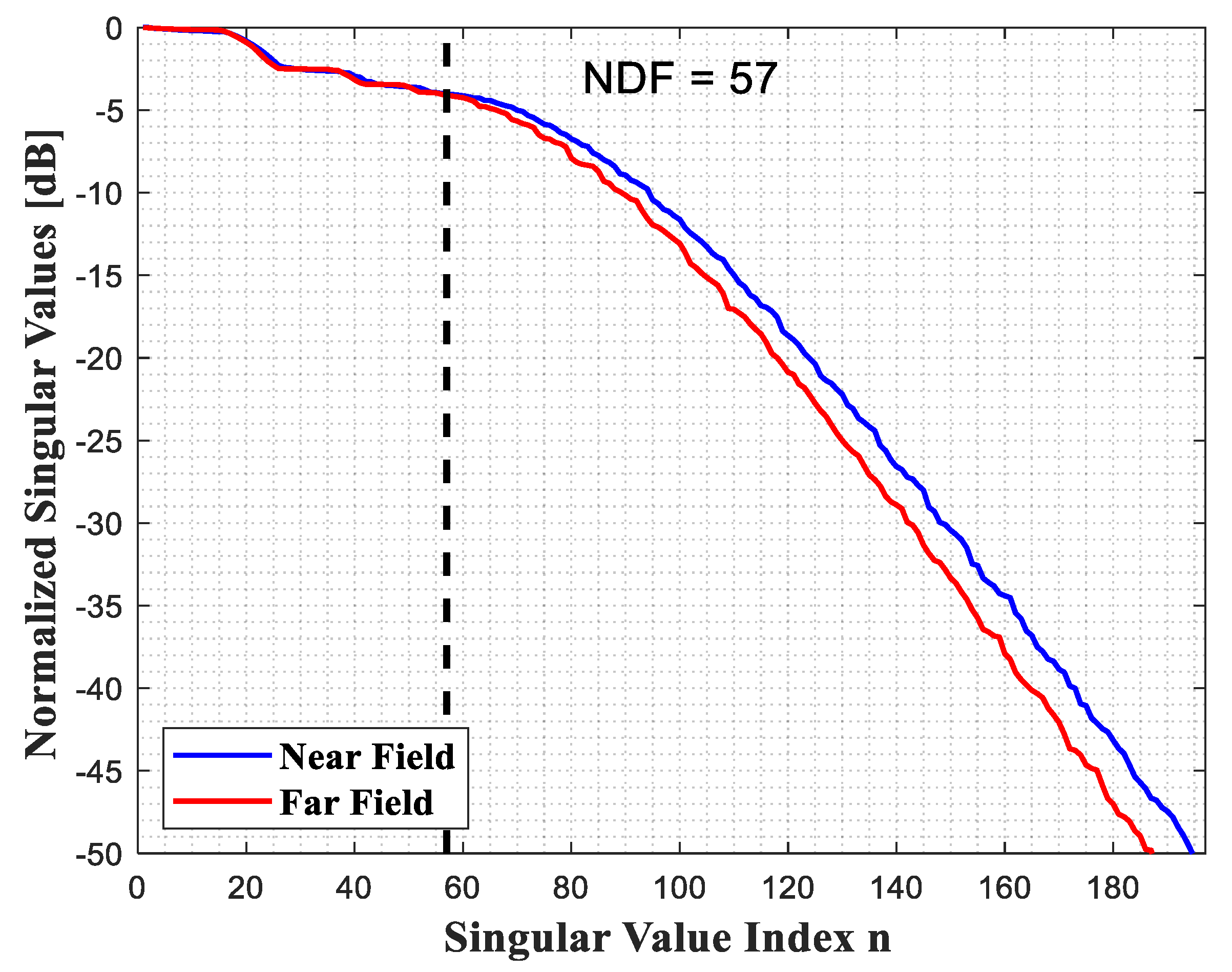
Figure 5 displays the behavior of the computed singular values of the pertinent operators for the near and far fields. It is observed once again that both NDFs are approximately the same, although their behaviors are different. (See
Appendix A for an explanation of this result for the present scenario).
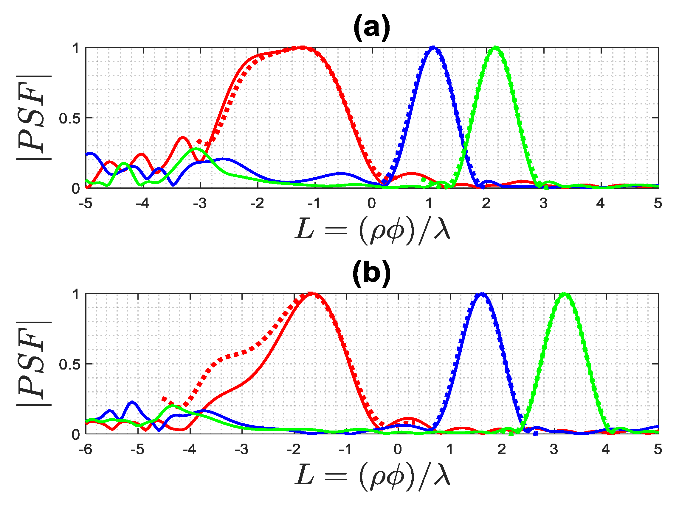
Figure 6 presents a comparison between the normalized amplitude of both PSFs along
-cut, achieved for different
values. We considered that three different point-like scatterers are positioned within the angular domain. Along the
the PSF exhibits a narrow main lobe width at the center of the angular range (indicated by the red lines). However, as the point-like scatterer moves from the center towards the edge, the main lobe width increases. Conversely, for the three points located well inside the ID (
), the main lobe width appears broader, and as
increases, the width becomes narrower. These results demonstrate that the proposed approximation accurately predicts the achievable resolution for each point-like scatterer.
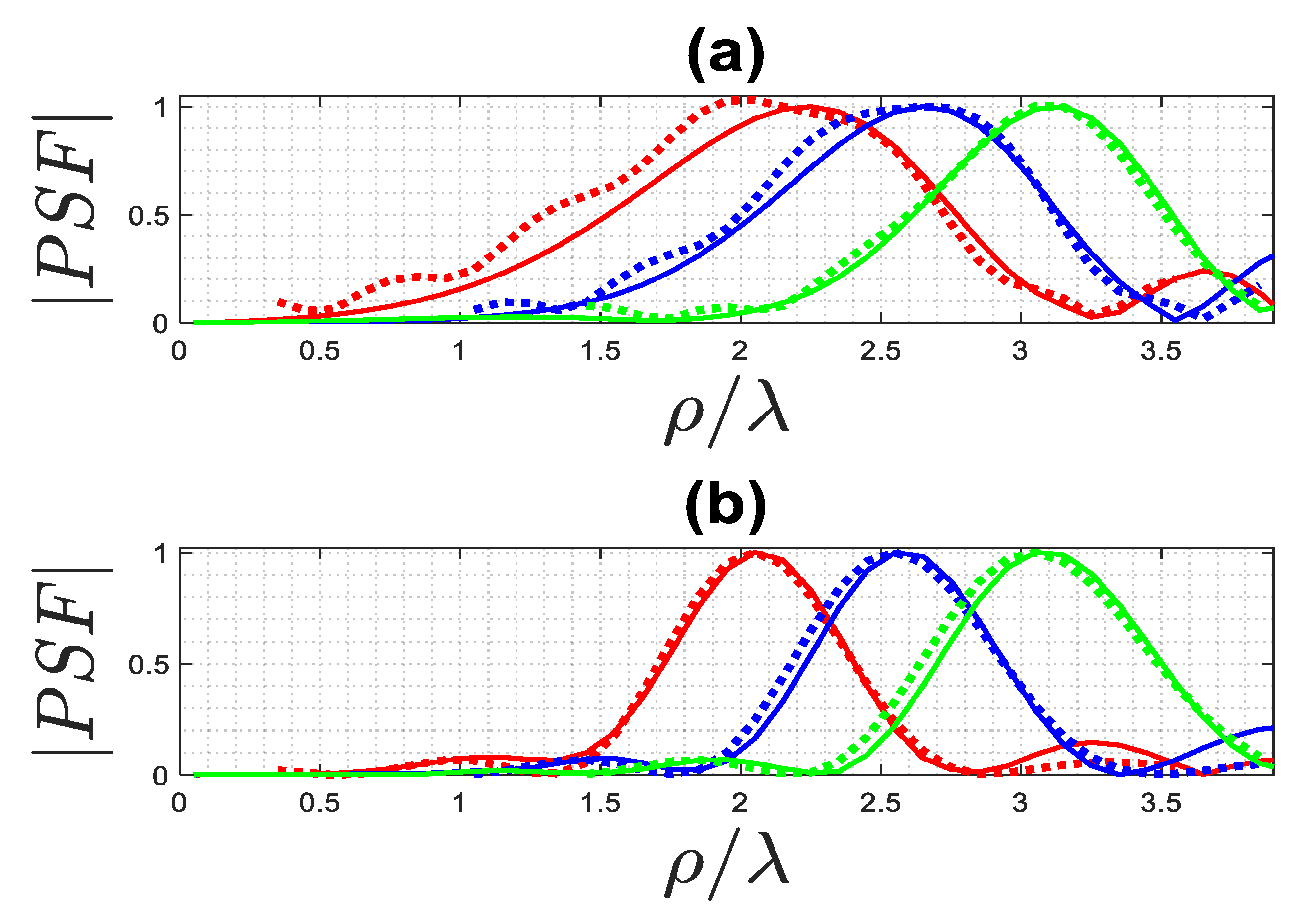
The previous example is replicated here for
(red lines),
(blue lines), and
(green lines) along
-cut for different
values, as shown in
Figure 7. Once again, it is observed that
, for the point-like scatterer located within the angular range, the main lobe width of their respective PSFs varies as their positions change. However, for
, which lies outside the angular range, the width of its main lobe becomes wide. Similarly, the width of the main lobe appears broad for three points situated at the depth of ID (
). Furthermore, increasing the
value results in a narrower main lobe width. These results once again verify that the approximation is acceptable for every point-like scatterer.
Figure 8 presents a comparison of two PSFs along the
-cut, aiming to evaluate the performance of the
and observe the achievable resolution. In
Figure 8a, the PSFs exhibit a wide main lobe width when
, while in
Figure 8b, the main lobe width is smaller when
. Along the
-cut, the resolution of the considered point-like scatterers remains constant but it varies as
changes. These results once again validate the effectiveness of the proposed
, which closely overlaps with the exact PSF for each point-like scatterer.
4. Application to Localization of Point-Like Scatterers
This section provides a localization application related to the theoretical discussions. The application concerns localizing some point-like scatterers. We consider a 2D full square dielectric object as an ID, where
and
, with
and
are equal to
. The ranges
,
and other parameters are the same as in the previous section. As mentioned earlier, the NDF for this ID is not available in the close form for the near scattered field. However, as discussed above and in the
Appendix A, the NDF can be expected to be approximately the same as the far scattered fields, which can be analytically derived from (17), and is given by
.
Figure 9 shows the normalized behaviors of singular values of relevant operators in the near and far fields and confirms that the NDF in the near field is approximately equal to the NDF in the far field for the same angular ranges of the position of sources and receivers.
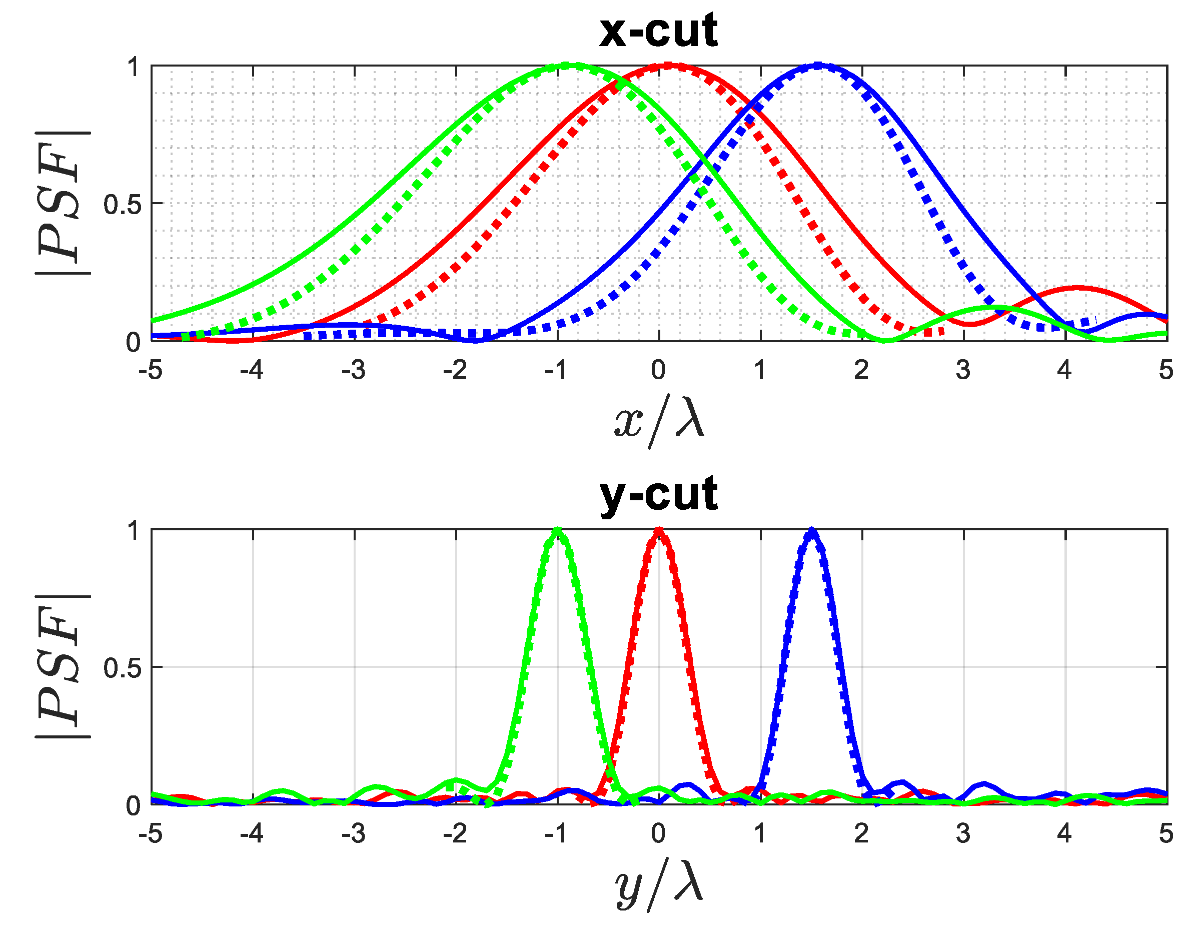
To implement our proposed application, it is necessary to determine the achievable resolution. For this purpose, a comparison between the exact and approximated PSFs is now provided along both the x-cut and y-cut, as depicted in
Figure 10. The results reveal that the main lobe width of the PSF along the x-cut is wider compared to the width of the main lobe in the y-cut. Consequently, the space-variant behaviour of the PSF is only observed when the scatterer moves from one cut line to another. In other words, the resolution remains unchanged along each cut. Additionally, the PSF results confirm that the approximated PSF can work well. We define the resolution, denoted as
, as half of the width of the main lobe of the PSF. Hence, the resolution
is determined as
along the x-cut, while the resolution
is measured as
along the y-cut.
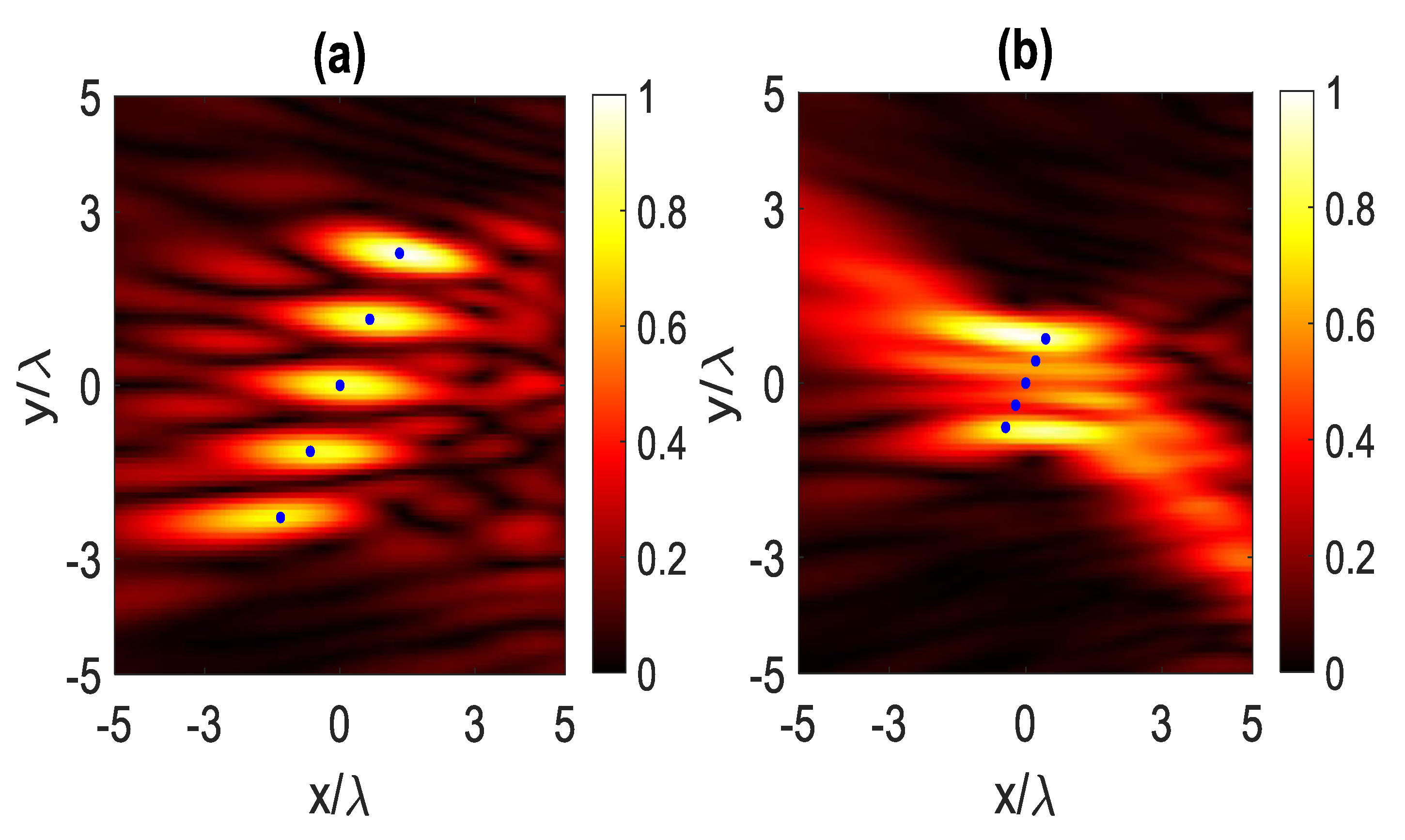
In this application, we consider the scenario where five point-like scatterers are positioned along an oblique line within the ID, which can mimic a localization problem along the separation between media with very different permittivities so that the PO approximation holds as sometimes in remote sensing. The reconstructed result of these point-like scatterers is displayed in
Figure 11.
Figure 11a validates that the considered scatterers are effectively resolved and can be distinguished from each other when they are spaced according to the resolution distance
. However, if the scatterers are located closer than the resolution distance
, as depicted in
Figure 11b, the reconstruction appears as two merged points instead of separate individual points.
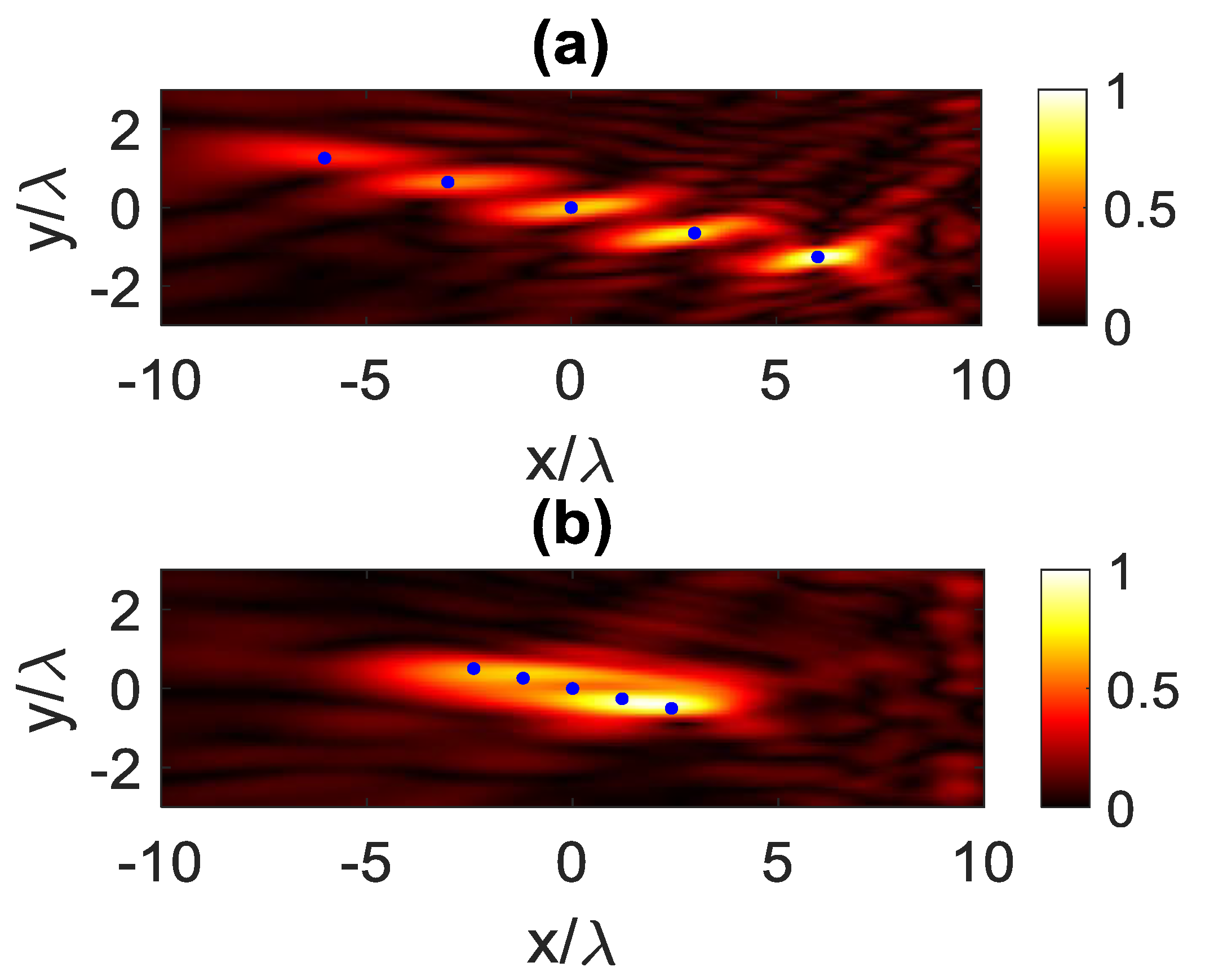
Since the resolution does not depend on the shape of the ID and as shown in the previous example
is large, therefore, we consider a rectangular geometry with
and
to reconstruct five point-like scatterers located on an oblique line within ID. In this case, the NDF is equal to 68 (which is computed by the equation provided in the previous example).
Figure 12 shows the reconstructed image of the considered points. When the distance between points is equal to the resolution
, they can be resolved well, as shown in
Figure 12a. On the other hand, if they are positioned at a distance less than the resolution, they appear as a line rather than separable points, as shown in
Figure 12b.
In conclusion, the defocusing effect of the PSF can be appreciated by the fact that the correct reconstruction of the same number of point-like scatterers can be achieved only when they are sufficiently spaced away, due to the width of the main lobe of the PSF according to observation and source locations. Additionally, this effect varies along different directions.


