1. Introduction
Subsurface microwave imaging aims at reconstructing a buried scattering scene from electromagnetic scattered field measurements [
1,
2]. This is a classical inverse scattering problem that finds application in many contexts, such as civil engineering diagnostics [
3,
4,
5,
6], archaeological and geophysical prospecting [
7,
8,
9,
10,
11], cultural heritage monitoring [
12], mine and improvised explosive device (IED) detection [
13,
14,
15] and, in general, in all cases where conducting non-destructive diagnostics is convenient or mandatory [
16].
From a mathematical point of view, subsurface imaging entails addressing an ill-posed non-linear inverse problem [
17]. Although a large body of work on “quantitative” reconstruction methods that deal with the non-linearity of the problem has been produced, their employment in realistic cases is somewhat limited since the main issues related to non-linear inversion—that is, converge issues, false solutions and computational costs—still represent significant challenges, especially when large (in terms of the wavelength) spatial areas have to be imaged [
18]. Moreover, in many cases, subsurface imaging is required to detect and localize the buried targets, i.e., mainly, it must provide “qualitative” reconstructions of the scene. Reconstruction methods based on linearized scattering models can be employed in these cases, with apparent advantages against the mentioned drawbacks affecting non-linear inversions.
Under a linearized scattering framework, the imaging problem is simplified since it amounts to inverting a linear integral operator called a scattering operator [
19,
20]. Moreover, the achievable performance can be linked to the features of the problem relatively easily [
21]. The achievable performance generally depends on the configuration [
22] (measurement aperture, stand-off distance, frequency band, strategy adopted for data collection), the background medium’s electromagnetic characteristics [
23], the noise level and the employed inversion algorithm [
24].
In this framework, the quantity of data collected is of paramount importance, since “too many” data do not necessarily improve the performance and can waste resources, whereas “too few” can lead to reconstructions crowded with artefacts, which can impair the detection of the actual targets. Thus, it is of great interest to devise a sampling scheme that requires a smaller quantity of data but, at the same time, preserves the performance in the reconstructions. Finding a proper sampling strategy is also relevant to reduce the cost/complexity of the Ground Penetrating Radar (GPR) system [
25]. GPRs are radar systems properly conceived to address non-destructive imaging and generally work near the interface between the air and the medium under investigation. However, recent developments have shown many advantages in using non-contact GPRs—for example, with GPRs mounted on a flaying platform [
26,
27]. In these cases, the spatial data sampling determines the trajectory—for example, in terms of the number of times that the radar needs to pass over the investigated area [
28] or the number of flaying platforms that must populate the fleet in the case of a multistatic configuration [
25].
Finally, sampling the data space is necessary to translate the continuous scattering problem into its finite-dimensional counterpart. Therefore, the number of data and their arrangement on the measurement domain affect the eigenspectrum of the discretized version of the scattering operator. Since the latter is related to the main metrics that allow us to quantify the performance in linear inverse problems, the number of data and their arrangement affect also the achievable performance and the resilience against noise. Generally, data sampling can be cast as a sensor selection problem [
29]. In particular, to avoid the related combinatorial complexity, several methods based on convex optimization [
30], greedy approaches and heuristics [
31,
32,
33] have been proposed. These methods select the measurement points by optimizing metrics related to the mean square error, the frame potential, etc., but require running iterative procedures, which could be cumbersome for a large-scale problem.
The selection of the measurement points can be achieved by properly considering the properties of the linearized scattering operator, so that no iterative procedures are required. For example, by expanding the Green function of the scattering operator in terms of its plane-wave spectrum (PWS) and neglecting the evanescent contribution, it can be easily shown that the scattered field can be sampled with a spatial step only depending on the wavelength. The resulting number of measurements is generally huge and not related to a priori information on the scattering domain. By employing stationary phase arguments [
34,
35,
36], the extent of the spatial region to be imaged is taken into account. This leads to a spatial sampling step that is generally larger than the one returned by the PWS argument. Hence, many data points are saved.
More recently, we progressed in the sampling theory by introducing the so-called warping approach [
37,
38]. It was shown that this method could consider the spatially varying filtering introduced by the near-field propagator. In more detail, it is shown that by introducing the so-called “warping variable”, mapping the scattering domain spatial variable
x into a new one
, the point-spread function (the reconstruction of the pulse scatterer) can be expressed as a band-limited function. This has two consequences. First, due the non-linear relationship between
and
x, the achievable resolution is spatially variable [
23]. Second Fourier arguments can be exploited to discretize the point-spread function returning in a uniform step in the spectral variable
w. The latter is non-linearly related to the spatial observation variable
, resulting in the non-uniform arrangement of the sampling points on the measurement domain. However, depending on the configuration parameters, the number of the required spatial data points is generally much lower than the one returned by the previous approaches [
34,
35,
36].
Previous contributions have detailed theories concerning the warping sampling method for different background media [
39,
40]. However, in these contributions, only relatively simple numerical examples were exploited to check the effectiveness of the warping sampling. In this paper, we provide the experimental validation of the latter, by considering a realistic subsurface scattering scenario concerning a water pipe buried under the soil. Essentially, our aim is to show that if experimental data coming from a typical subsurface scenario are collected on the non-uniform grid returned by the warping sampling strategy, the reconstruction results are very close to the ones returned by processing a very large number of measurements. This means that the proposed strategy succeeds in reducing the number of data compared to the literature, without significantly affecting the reconstruction results. While the warping approach applies regardless of the stand-off distance, here, we collect the measurements through a commercial GPR that slides over the air/soil interface in order to synthesize the measurement aperture. We consider to collect the data along a pathway leading to a fountain in a cloister near our Engineering Department, below which a water pipeline is presumed to be buried. Moreover, the 3D scattering scene is reconstructed by a slice approach that interpolates a collection of 2D inversions [
41]. Although the 3D Green function should be considered even in the slice reconstructions [
42], for the sake of simplicity, each slice is addressed as a 2D scalar inverse problem. This approximation works because the water pipeline is elongated along one direction.
The rest of the paper is organized as follows. In
Section 2, the mathematical formulation of the problem is briefly introduced, and the link between the achievable performance and sampling is established.
Section 3 is devoted to recalling some literature sampling criteria and presenting the basics of the warping sampling theory. However, we advise the reader that all the theoretical details of this approach can be found in [
37,
38,
39,
40]. In
Section 4, the scattering experiments are described, and the corresponding reconstructions are reported. Finally, conclusions and future developments close the paper.
2. Problem Description
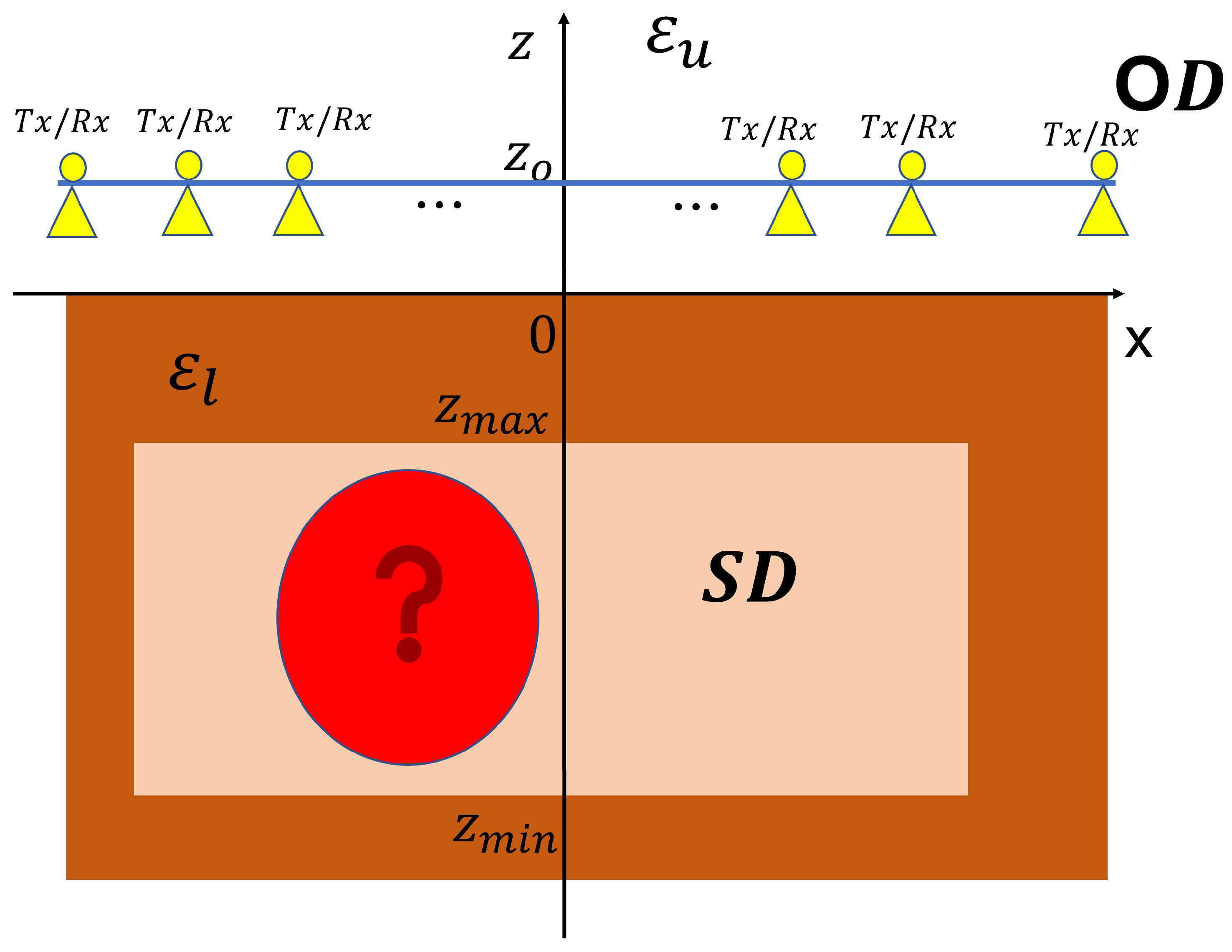
The single scattering slice is schematized as the 2D scalar scattering problem sketched in
Figure 1. Invariance is assumed along the
y-axis. The background is a two-layered medium consisting of two homogeneous half-spaces separated by a planar interface at
. The upper half-space is the free space and its dielectric permittivity is denoted by
, whereas the lower half-space represents the soil; it is electromagnetically denser then the free space and its dielectric permittivity is denoted as
. Both the half-spaces are non-magnetic so that the magnetic permeability everywhere is the same as that of the free space
.
The targets to be detected are buried in the lower half-space. In particular, imaging is achieved by looking for the targets within a bounded rectangular spatial region
, with
, addressed in the following as the scatterer domain. A larger spatial region can be conveniently addressed, for example, by employing the zoom approach presented in [
43]. The transmitting antenna radiates an incident field linearly polarized along
y at different frequencies within the wavenumber band
, with
being the wavenumber in the free space. A monostatic configuration is considered, so that the scattered field is collected at the same position as the source, while the latter moves to synthesize the measurement line. In particular, for the single slice reconstruction, the measurement domain consists of a linear domain
of the
x-axis located at some height
above the separation interface from the free-space side.
By linearizing the scattering phenomenon according to the Born approximation [
44], the buried targets and the scattered field collected over
are linked through a linear integral operator
where
and
represent the sets of square integrable functions supported over
and
, respectively;
is the so-called contrast function, with
being the dielectric permittivity of the unknown scatterer. It is remarked that (
1) is a rather general mathematical framework to describe the scattering phenomenon. Indeed, if it is a priori known that the contrast function enjoys some smooth/regular behavior, then more “narrow” function sets can be chosen for the unknown space; for example,
X can be assumed to be a Sobolev space. Instead, this does not hold true for
Y, since noise, and uncertainties in general, always corrupt the measurements.
In detail, the operator
is given by the following expression:
where
,
,
is the angular frequency;
is the wavenumber in the lower half-space medium, with
being the refractive index; and
is the Green function of the two-layered background medium. Note that the Green function appears squared because of the considered monostatic configuration. Moreover, the dependence on
is omitted since the measurement line is deployed at a constant height from the interface.
By assuming that
,
being the wavelength in the lower half-space, the Green function can be approximated as
where
accounts for the amplitude and
the phase changes occurring while propagation takes place. In particular, having denoted as
and
the target and the field points, then
and
are the paths traveled by the waves in the upper and lower half-spaces, respectively, and
is the refraction point at the separation interface given by Snell’s law as
In particular, if the measurement line is located over the separation interface, then , , and the phase term simplifies as , with . In other words, the phase term is the same as propagation in a homogeneous medium with the properties of the lower half-space.
Inversion and Sampling
Radar imaging entails inverting Equation (
2) for the
function in order to obtain images of the subsurface region. For example, let us say that
is a reconstruction operator that, starting from the data field, returns an estimation of the unknown contrast, which is
In the case of a point-like target, i.e.,
, (
6) returns the so-called point-spread function (psf)
. Therefore, because of the linear formulation, the psf provides the link between the unknown and its reconstructed version as
Equation (
7) highlights that the contrast function, during the reconstruction process, undergoes filtering that is dictated by the psf features, which in turn depend on the parameters of the configuration and, in general, on the adopted inversion scheme (which is
) in conjunction with the noise level.
Since the psf dictates the performance achievable in the reconstructions, a natural means to set the sampling strategy—and, at the same time, to preserve performance—is to sample the data so as to approximate the point-spread function in (
7), corresponding to the ideal (unfeasible) case in which data are collected continuously over
.
As mentioned above, the psf can depend on the inversion algorithm that one wishes to apply. Let us further consider this important point. In principle, a psf behaving similarly to a Dirac delta is desired since this would entail perfect reconstructions. In practice, this is not possible because of the unavoidable presence of noise/uncertainties in the data and the ill-posedness of the imaging problem. In order to obtain “meaningful” reconstructions, regularized inversion schemes must be exploited [
24,
44]. Hence, the psf, in general, depends on the used regularization strategy.
Nonetheless, to devise the sampling strategy, we conveniently consider a simple adjoint inversion method. Accordingly, we denote as
the adjoint operator of
. Its explicit expression is given by
with
denoting conjugation. In particular, by invoking the same Green function approximation as in (
3), expression (
8) becomes
The reconstruction is then given by
where the subscript
merely indicates that inversion is achieved by the adjoint operator.
Some remarks are in order to justify our choice. First, it is clear that (
10) is a type of backpropagation [
45,
46] because phase conjugation appears in the kernel of
. Furthermore, the corresponding point-spread function, i.e.,
with
, is exactly the kernel of the operator
. It then follows that devising the sampling scheme so as to approximate (
11) is a means to approximate the singular system,
, of
as well. Now, it is observed that any regularized inverse scheme can be cast as an inverse filtering procedure [
24], i.e.,
where the filtering is dictated by the windowing sequence
, which in turn depends on the chosen regularization strategy. As a consequence, finding a sampling strategy with the aim of approximating (
11) will work regardless of the employed inversion method.
3. The Warping Sampling
In the previous section, we concluded that devising a data sampling strategy is equivalent to finding a proper quadrature role to approximate the integral representation of
. In the event that the measurement domain is in the far field [
47], or even when the Fresnel paraxial approximation works [
28], the matter is relatively straightforward, since the scattering operator can be given in terms of a Fourier transform and the data can be sampled according to the Nyquist sampling rate. When far-field conditions or the Fresnel approximations do not hold, the spatial frequency band of the scattered field can be estimated by invoking stationary phase arguments and the Nyquist step set accordingly (as shown in [
34,
35,
48]). In these contributions, it was correctly pointed out that, due to the near-field configuration, the frequency band of the scattered field is changed upon changing the target position within the investigated area. In other words, the data frequency band is spatially varied. We denote such bands as
, with
. Note that the maximum employed wavenumber (i.e., the maximum working frequency) is considered in the
B estimation. In order to achieve uniform sampling, the data frequency band is usually overestimated as
and this leads to an unnecessarily large number of spatial measurement points.
Recently, we introduced the warping sampling approach, which properly takes into account the spatially varying nature of the data frequency band [
49]. It was proven that the measurement positions are non-uniformly arranged but their number can be significantly reduced as compared to other sampling strategies [
37,
39]. Below, we give a brief description of such a sampling method.
In principle, data reduction requires one to optimize the spatial sensors’ positions and the frequencies at which measurements need to be collected. However, here, we consider the determination of the spatial sampling only. This is because optimizing the frequency sampling as well can lead to cumbersome configurations where the spatial positions change for each selected frequency [
47]. Therefore, the sampling of the wavenumber band is achieved by employing standard arguments based on the range extent of the area to be imaged, i.e.,
. We denote as
the corresponding sampled frequencies. Thus, (
11) is approximated as
with
To devise the spatial sampling, we need to focus on
. In particular, to establish a sampling approximation that works for each frequency and for each position within the investigation domain
, in (
14), we set
and
, since the spatial frequency band of the scattered field is larger for targets that are closer to the observation domain and in correspondence to the highest adopted frequency. Accordingly, (
14) is particularized as
where the dependence on
z is understood since, as mentioned above, it is constant and set as
. Now, a warping transformation
is used to stretch the interval
into
.
is a degree of freedom that can be chosen at convenience, provided that it is monotonic. The next step is to rewrite the phase term in (
15) by employing the first-order integral form of the Taylor remainder as
with
and
and
. The function
is continuous and monotonic decreasing with respect to
, and hence invertible,
(see [
39]). Therefore, integration in
can be replaced with integration in
w. In more detail, by denoting
and
by setting
, the expression of
can be rewritten as
where
. Note that
and
depend on
and
, which clearly shows the spatially varying behavior of the point-spread function mentioned above.
By choosing the warping transformation
as [
23]
and considering the amplitude term evaluated in correspondence to the leading-order term occurring for
, (
20) is recast as
It is seen that as a consequence of the warping transformation (
21), the bandwidth
is now constant and equal to 1, so that the spatially varying behavior mentioned above is now embodied in the non-linear link between
x and
. Moreover,
is arranged as a pseudodifferential transformation [
50]. Accordingly, the Horiuchi [
51] approach can be employed to set the sampling scheme. As detailed in [
39], the resulting sampling law is given by
with
being the
m-th sampling point. Accordingly, the required number of spatial samples (to be deployed non-uniformly, although symmetrically) is found to be
where it is shown to be much lower than the number of spatial samples required by all other criteria described in the literature when near-field configurations (as for the case at hand) are considered [
37,
38,
39]. Note that all the sampling criteria in the literature refer to a free-space configuration. Accordingly, the comparison is pursued when
, where, for the sampling point estimation, the background medium can be assumed to be homogeneous and equal to the lower half-space.
4. Experimental Results
In [
37,
39,
40], some numerical examples are provided that show how the warping sampling method reduces the number of data without affecting the reconstruction performance. However, each theoretical approach must pass experimental verification to prove its effectiveness. To this end, in this section, we apply the warping method to a real subsurface imaging scattering scenario.
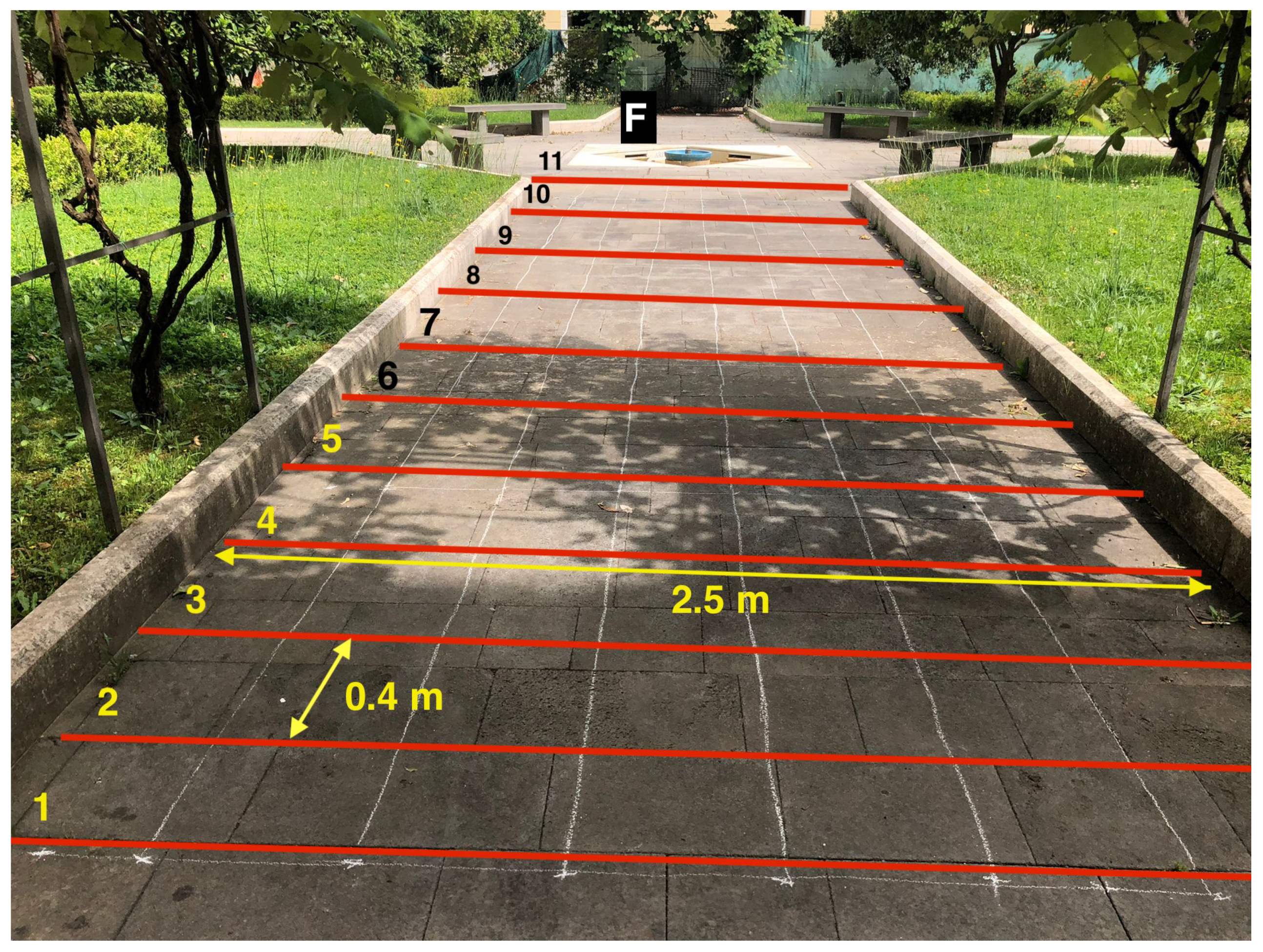
The experimental measurement setting is shown in
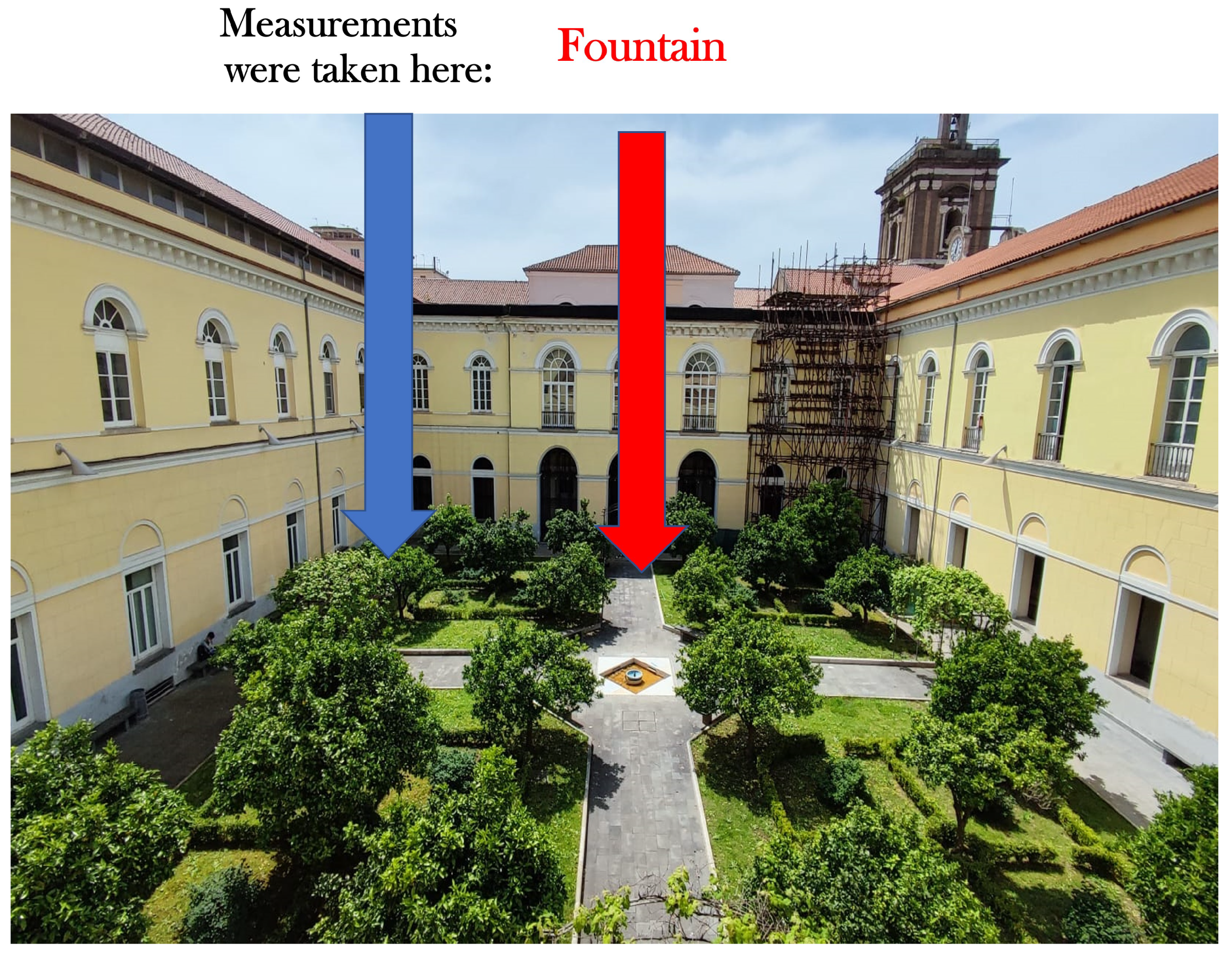
Figure 2. In particular, we consider a pathway leading to a fountain in a cloister near our Engineering Department (see
Figure 3), below which a water pipeline is presumed to be buried. The red horizontal lines indicate the measurement domain in the pathway. The measurements are taken over eleven lines spread over
m. The observation domain for each measurement line is
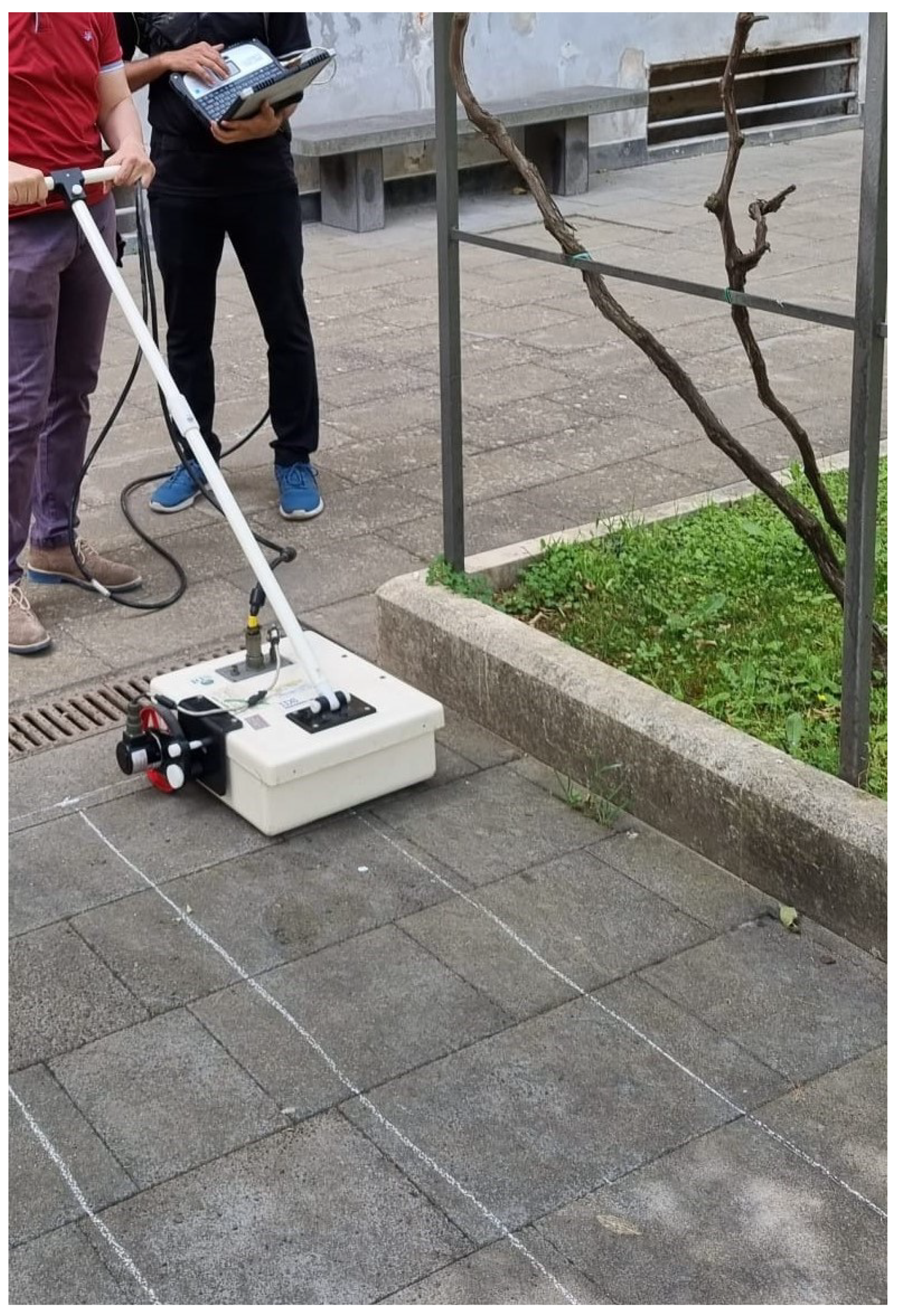
m long. An IDS RIS-K2 Georadar is used for data acquisition (see
Figure 4). The GPR system used for the scattered field measurements emits a Ricker pulse centered at 200 MHz, and the data are collected with a spatial step of
m. It must be stressed that the mentioned spatial step is much below what the warping prescribes. This is implemented to obtain a benchmark against which to compare the data reduction achieved by the warping sampling. This dense data set will be addressed as the oversampled data set in the following.
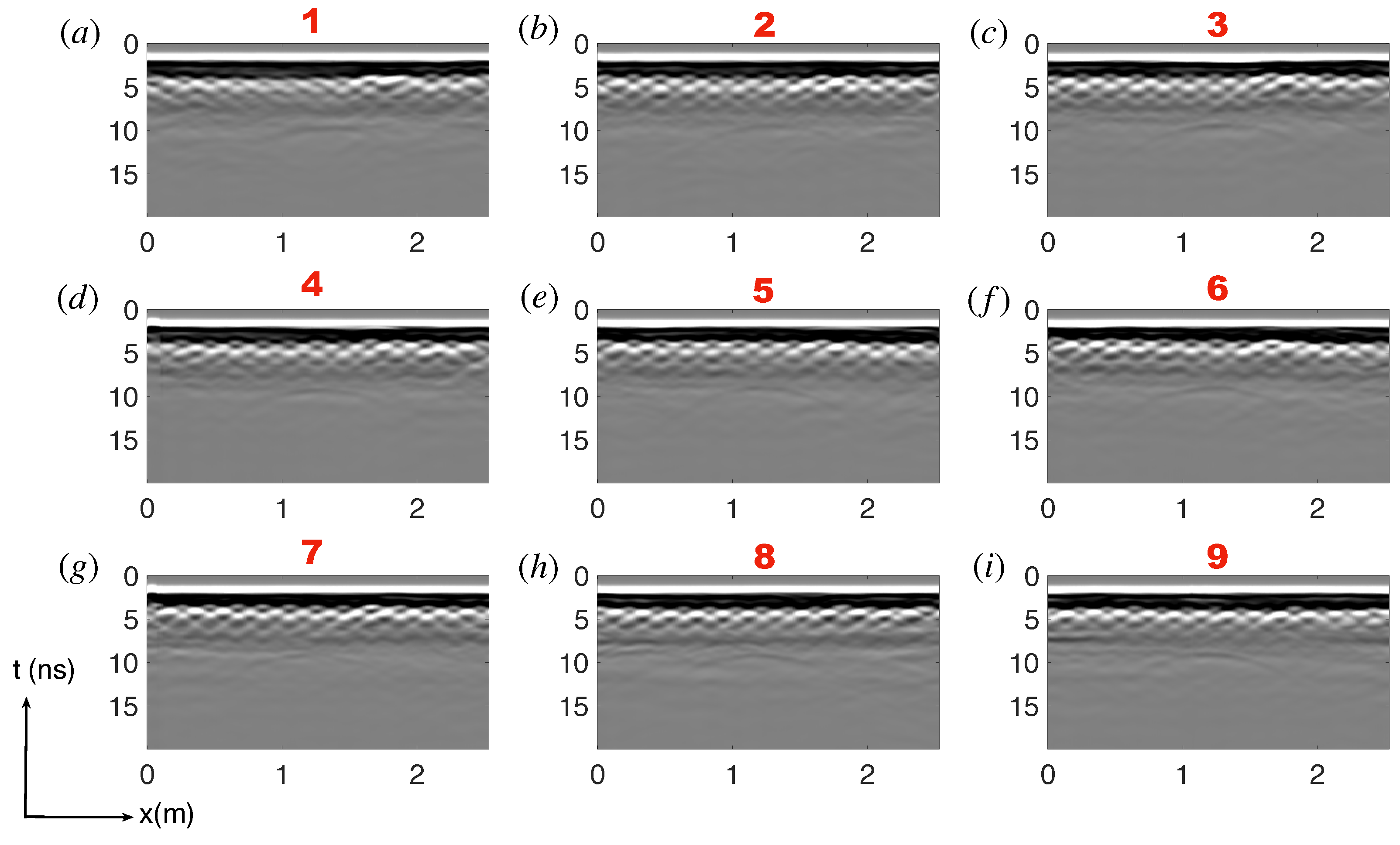
The scattered field measurements for measurement lines from 1 to 9 are shown in the radargrams reported in
Figure 5. Raw measurements must be pre-processed to remove clutter from GPR internal reflections and the ground interface. To this end, the literature provides various methods for ground clutter rejection, such as the mean subtraction method [
52,
53,
54], the subspace projection method [
55], etc. These methods remove the clutter but tend to partially filter the already weak signals coming from buried targets. It is better to remove clutter using a time gating procedure to avoid this adverse effect. In particular, here, we use the entropy-based time gating method presented in [
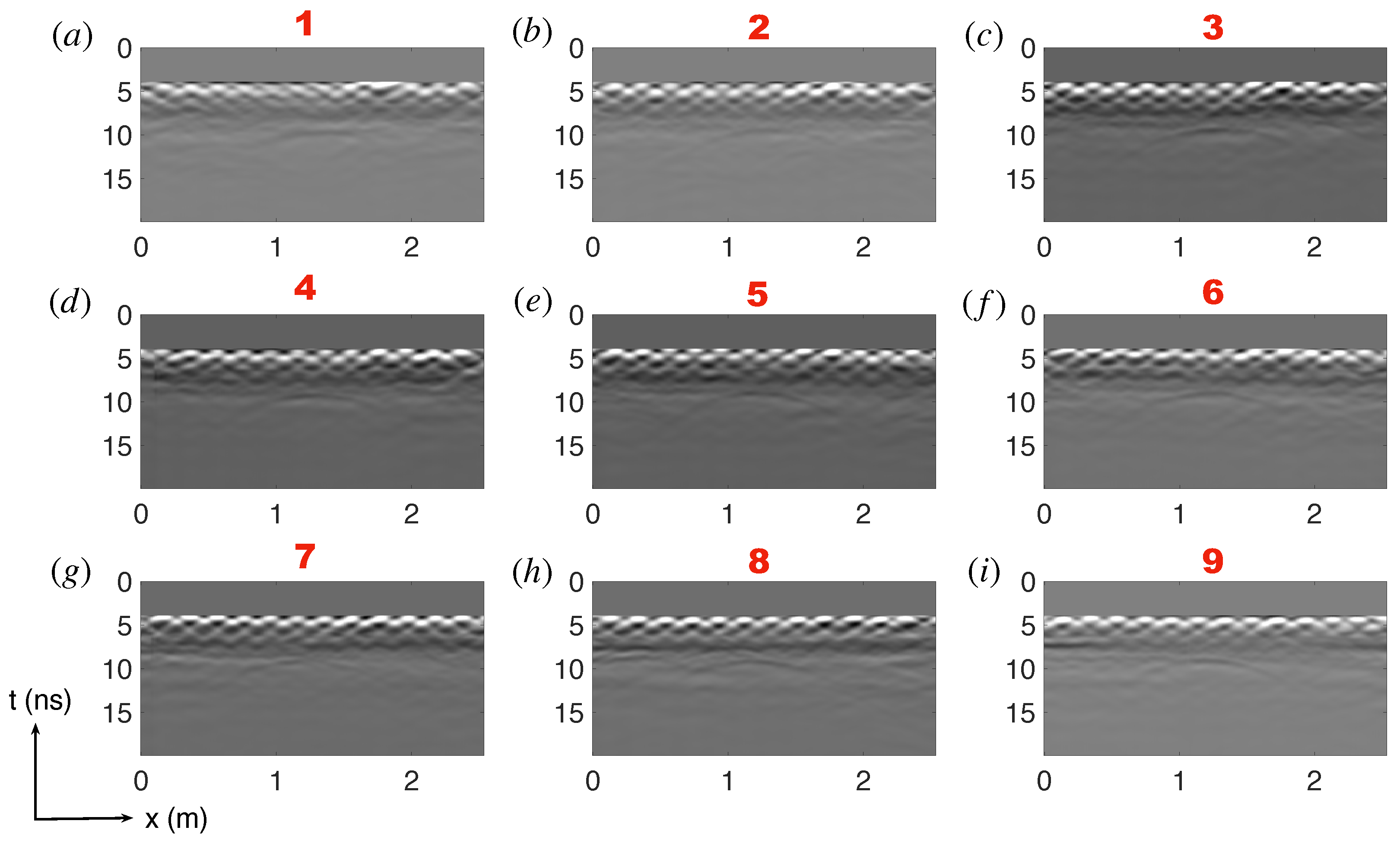
56]. In more detail, the entropy measures the similarity of the reflected signal collected by the different time traces over the length of the measurement domain. At a given instant, the reflected signal is classified as clutter if the entropy is high, meaning that high similarity occurs. A time gating window supported over the interval of times with low similarity is set and multiplied with each trace of the measured signal so that the ground interface and antenna’s internal reflections are eliminated. The pre-processed measurements are shown in
Figure 6 after clutter rejection.
The radargrams in
Figure 6 show that the scattered signals mainly consist of many shallow buried hyperbolas and less strong hyperbolas almost in the middle of the pathway and more deeply located. This is consistent with the presence of a reinforcement grid located very close to the air/soil interface and a pipeline supplying water to the fountain.
To obtain the reconstructions, the time traces are Fourier-transformed and frequencies within the band 100–800 MHz are retained with a frequency step of 25 MHz. Accordingly, the collected data for each measurement line are
, where
M and
refer to the spatial and frequency samples, respectively. This is the oversampled data set. By contrast, the warping method requires
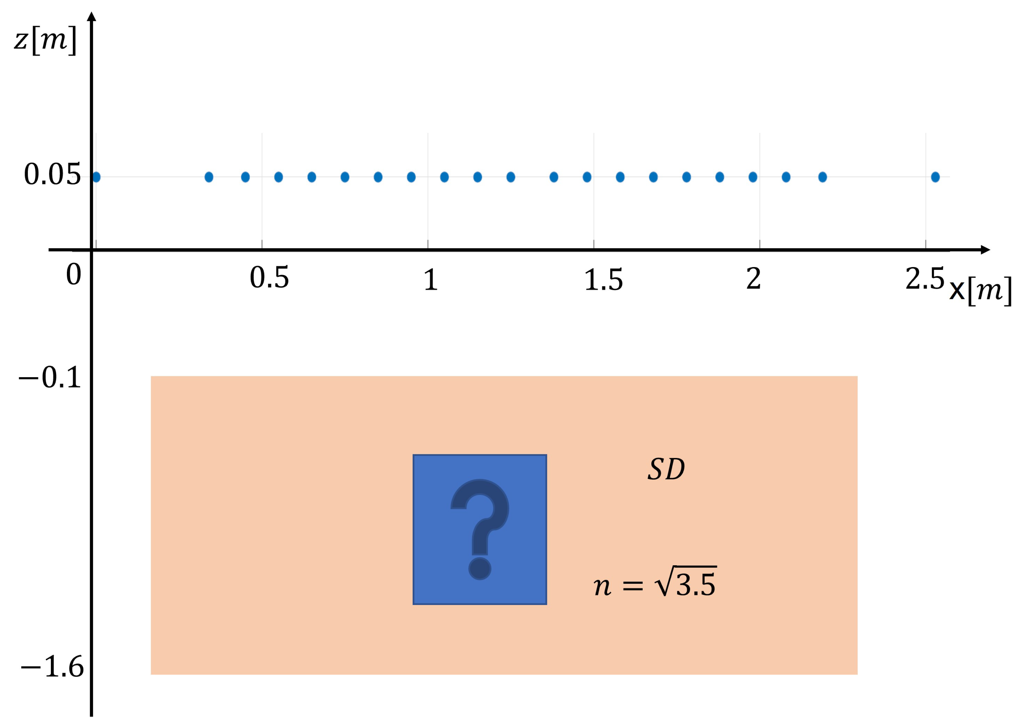
data. The corresponding spatial layout of the measurement points is shown in
Figure 7. In particular, the measurement grid is obtained from (
23) by assuming that the lower half-space has relative dielectric permittivity of
and by considering
m and the scattering domain
, so that
and
for each slice. Note that to derive (
23), we assume that
and the x-axis of
are symmetric with respect to the origin. The latter is not a limitation because the points can be derived for a symmetric reference system and then translated into a non-symmetric one. As can be seen from
Figure 7, the measurement points are non-uniformly arranged on
; in fact, the sampling step is low at the center and it enlarges as the measurement point approaches the edge of
. To point out the actual data reduction brought about by the warping approach, we observe that, for the case at hand, if the sampling criterion introduced in [
34,
35,
36,
48] is employed, then the required spatial measurement points would be more than four times the ones returned by the warping. In general, for near-zone configurations, warping always requires fewer spatial data, with the reduction ratio depending on the scattering configuration (see [
39] for more comparative analyses between warping and the sampling approach introduced in [
34,
48]). According to previous arguments, we can conclude that the warping sampling allows for a dramatic reduction in the number of spatial measurements. Note that this reduction is even greater if all nine slices are considered.
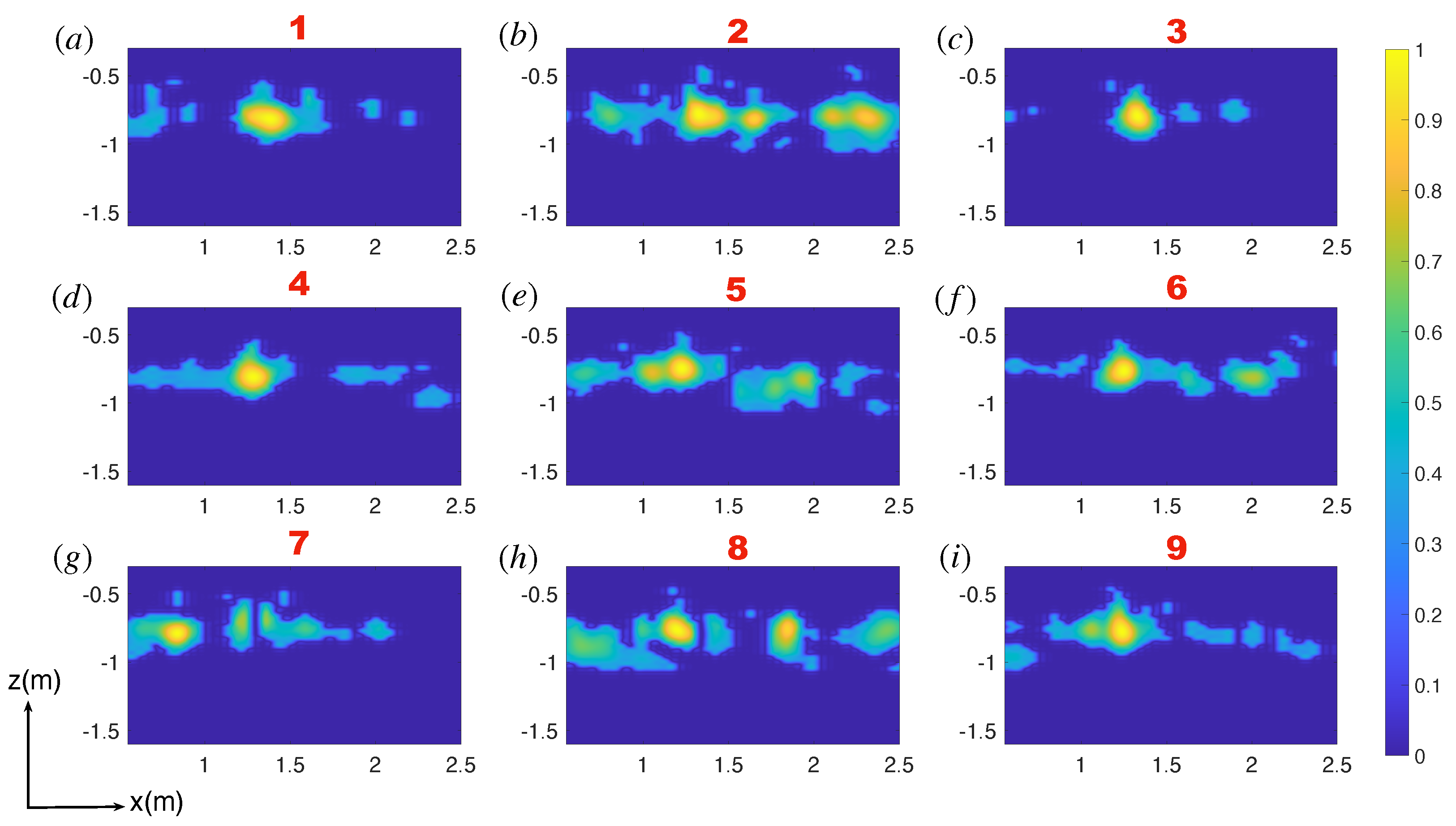
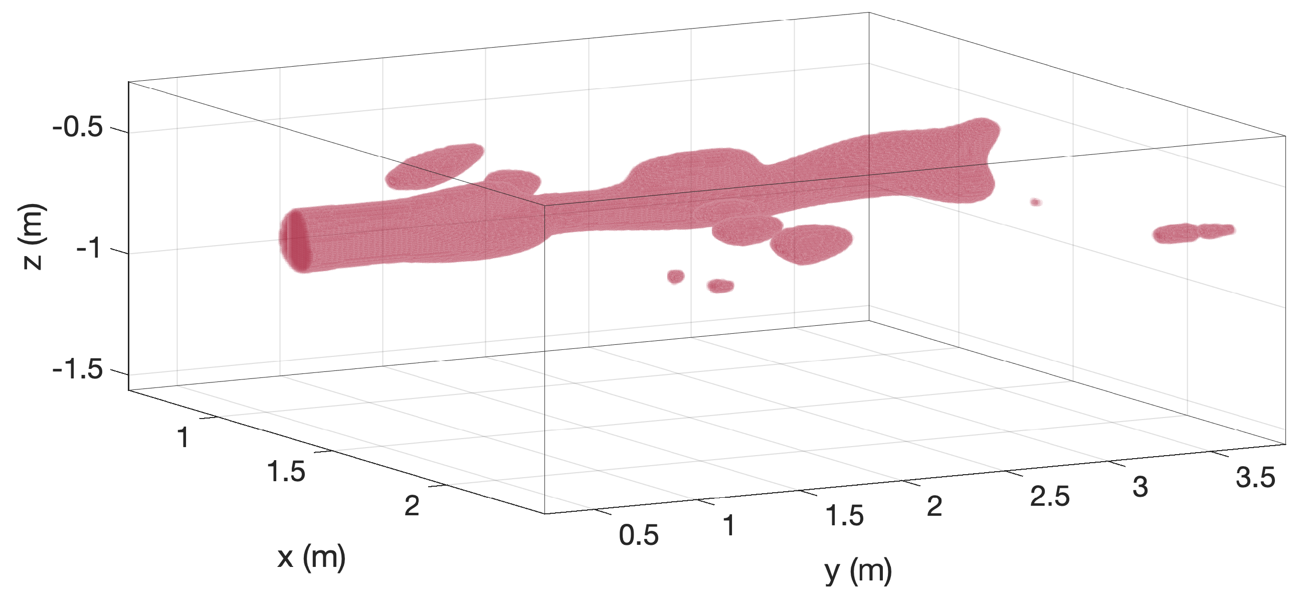
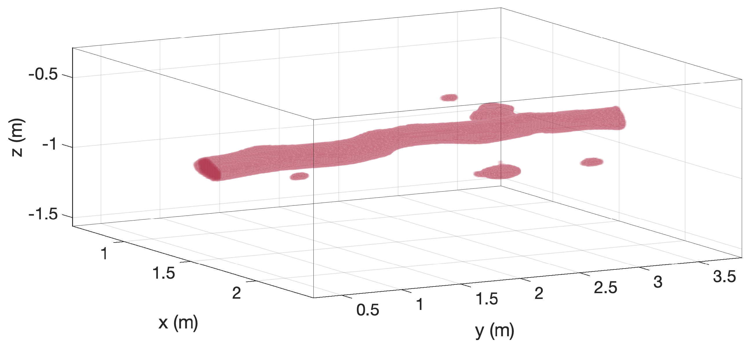
However, we still need to check the achievable performance in the reconstructions. To this end, the scene reconstruction is pursued by a slice approach: for each measurement line, a 2D slice of the scene is obtained. Then, the slices are interpolated and shown as a 3D isosurface plot. For each slice, is discretized into pixels. Furthermore, slice reconstructions are obtained by the backpropagation algorithm based on the matrix version of the adjoint of the scattering operator, as recalled above.
As noted above when inspecting
Figure 6, there are two main buried targets: the shallow grid and the more deeply buried pipe. Therefore, for a clearer display of the reconstruction, the overall buried region is split into two parts: the region very close to the interface and the deeper subsurface. In the following, we report all the reconstructions corresponding to the deeper region, where we aim to detect the buried pipe.
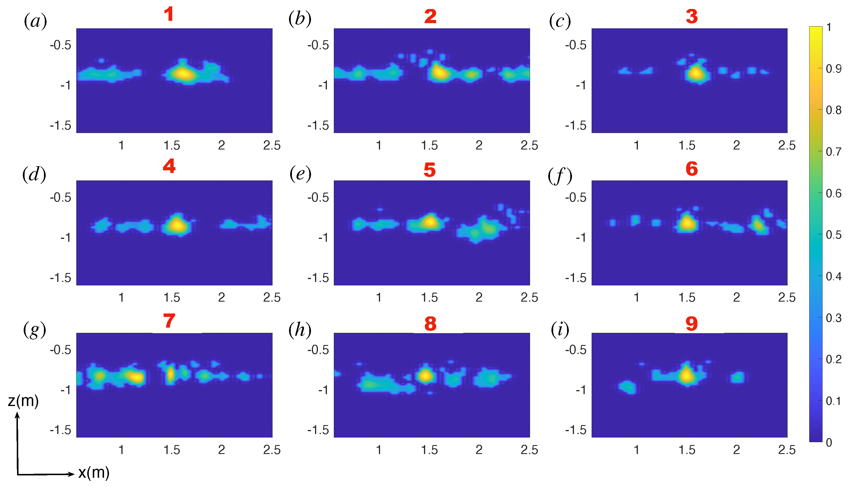
The normalized slice reconstructions (from slice 1 to 9) are reported in
Figure 8 and
Figure 9. In particular, in
Figure 8, the measurements are collected according to the oversampled set.
Figure 9 shows the reconstruction results when data are collected on the non-uniform grid shown in
Figure 7 returned by the warping approach. In both cases, a detection threshold of
is employed. The corresponding 3D interpolated reconstructions are instead displayed in
Figure 10 and
Figure 11. As mentioned above, due to the linear scattering model exploited in this paper, only a qualitative reconstruction of the scattering scenario is expected to be achieved. However, this should be sufficient to detect and localize the buried targets. This is confirmed by
Figure 8,
Figure 9,
Figure 10 and
Figure 11. In fact, for both sampling strategies, we achieve a qualitative reconstruction that allows us to detect and localize the pipe. Moreover, by comparing
Figure 8 to
Figure 9, it can be observed that although some differences appear, the quality of reconstructions is comparable, and the buried pipe is, in both cases, clearly detected and localized. This is even clearer when considering
Figure 10 and
Figure 11. This definitively shows that the warping sampling method works effectively.
5. Discussion and Conclusions
The aim of this paper was to check the effectiveness of the warping sampling method in the case of a realistic subsurface scattering scenario. The presented analysis confirmed that the warping sampling allows for a significant reduction in the number of spatial measurements compared to other sampling criteria described in the literature, without compromising the quality of the reconstructions. This is a remarkable advantage since it allows us to use fewer sensors for real aperture radar systems or reduces the time for data collection in synthetic aperture radar systems. Moreover, the computational burden in obtaining the reconstructions and the required storage resources is also diminished. This is important, particularly as subsurface imaging deals with large spatial regions.
It must be stressed that for convenience and according to the available instrumentation, we considered a GPR working in contact with the air/soil interface. However, the theory behind the warping sampling is general and can be applied regardless of the stand-off distance and, in particular, to the case of a GPR mounted on a flaying platform. In the latter case, reducing the number of data to deal with could be even more important.
A key point that is worth emphasizing is that the warping method allows us to determine the spatial measurement arrangement analytically and explicitly takes into account all the main components of the problem, i.e., the extent of the measurement line, the size of the subsurface area to be imaged, the dielectric permittivity of the embedding half-space, etc. This is in contrast to other general-purpose methods addressed in the literature as sensor selection procedures. In fact, these methods are merely numerical and require some iterative procedure to select the sensors’ positions.
A slice approach addressed the subsurface imaging, and the warping sampling was applied only to each measurement line. In this way, the spatial sampling was addressed within the framework of a 2D imaging problem. One future development concerns the extension and the validation of the warping sampling in the entire 3D case. In this regard, we remark that the related dyadic nature of the involved scattering operator is not, in principle, a problem, since the Green function’s phase term plays a major role in sampling. A simple means to address the 3D case is to separately apply the warping sampling along the two transverse dimensions of the measurement aperture. While this would allow one to obtain a dramatic reduction in the spatial measurements (always compared to sampling strategies in the literature), it is a sub-optimal method to employ the warping. The reason is that for near-field configurations, the phase term of the Green function does not factorize with respect to the two transverse variables of the measurement aperture. Therefore, more involved warping transformations are required. Preliminary results in this direction have been presented in [
57].
A further point of interest that we plan to address as a future development is the case of more involved background media—for example, when it consists of a layered medium with more than two half-spaces.
Finally, we point out that warping sampling considers only spatial sampling, whereas the frequency is sampled by employing common Fourier-based arguments. In principle, there is room for further data reduction if the frequency sampling is optimized. However, as mentioned in the paper, this can lead to cumbersome measurement settings where the spatial positions change with frequency. Research activities are ongoing regarding this question and, in particular, to find a convenient solution to optimize the sample data in both the spatial and frequency domains.


