MS-AGAN: Road Extraction via Multi-Scale Information Fusion and Asymmetric Generative Adversarial Networks from High-Resolution Remote Sensing Images under Complex Backgrounds

Abstract

Extracting roads from remote sensing images is of significant importance for automatic road network updating, urban planning, and construction. However, various factors in complex scenes (e.g., high vegetation coverage occlusions) may lead to fragmentation in the extracted road networks and also affect the robustness of road extraction methods. This study proposes a multi-scale road extraction method with asymmetric generative adversarial learning (MS-AGAN). First, we design an asymmetric GAN with a multi-scale feature encoder to better utilize the context information in high-resolution remote sensing images (HRSIs). Atrous spatial pyramid pooling (ASPP) and feature fusion are integrated into the asymmetric encoder–decoder structure to avoid feature redundancy caused by multi-level cascading operations and enhance the generator network’s ability to extract fine-grained road information at the pixel level. Second, to maintain road connectivity, topologic features are considered in the pixel segmentation process. A linear structural similarity loss ($L_{SSIM}$) is introduced into the loss function of MS-AGAN, which guides MS-AGAN to generate more accurate segmentation results. Finally, to fairly evaluate the performance of deep models under complex backgrounds, the Bayesian error rate (BER) is introduced into the field of road extraction for the first time. Experiments are conducted via Gaofen-2 (GF-2) high-resolution remote sensing images with high vegetation coverage in the Daxing District of Beijing, China, and the public DeepGlobe dataset. The performance of MS-AGAN is compared with a list of advanced models, including RCFSNet, CoANet, UNet, DeepLabV3+, and DiResNet. The final results show that (1) with respect to road extraction performance, the Recall, F1, and IoU values of MS-AGAN on the Daxing dataset are 2.17%, 0.04%, and 2.63% higher than the baselines. On DeepGlobe, the Recall, F1, and IoU of MS-AGAN improve by 1.12%, 0.42%, and 0.25%, respectively. (2) On road connectivity, the Conn index of MS-AGAN from the Daxing dataset is 46.39%, with an improvement of 0.62% over the baselines, and the Conn index of MS-AGAN on DeepGlobe is 70.08%, holding an improvement of 1.73% over CoANet. The quantitative and qualitative analyses both demonstrate the superiority of MS-AGAN in preserving road connectivity. (3) In particular, the BER of MS-AGAN is 20.86% over the Daxing dataset with a 0.22% decrease compared to the best baselines and 11.77% on DeepGlobe with a 0.85% decrease compared to the best baselines. The proposed MS-AGAN provides an efficient, cost-effective, and reliable method for the dynamic updating of road networks via HRSIs.

1. Introduction

Remote sensing images acquired by airborne or satellite-based sensors are the main resource for earth surface observation, environmental monitoring, target identification, etc. [1]. Road extraction from remote sensing images has wide applications in urban management [2], traffic control [3], map updating [4], smart city [5], intelligent transportation [6], urban planning [7], autonomous driving [8], and emergency management [9], etc. Traditional road extraction methods are mainly through manual visual identification, which not only consumes huge human resources but also falls far short of data update requirements [10], and the error rate is relatively high according to the practices from the US government and related mapping companies [11]. Automatic road identification based on remote sensing images will significantly reduce labor costs and improve the efficiency and accuracy of road monitoring, providing an efficient, cost-effective, and reliable solution for the dynamic updating of road networks [12].

With the development of modern sensors on various satellite platforms such as IKONOS, QuickBird, and GeoEye, high-resolution remote sensing images (HRSIs) have become a common data resource due to the spatial, spectral, and temporal resolution in the domain of road extraction in recent years [9,13]. Automatic extraction of road networks from HRSIs provides a new way to access detailed geographic information on road network distribution [14].

Early methods are mostly based on prior knowledge from geometric, photometric, and textural perspectives of roads [15]. However, the classification accuracy is far from satisfactory due to misclassification between roads and other spectrally similar objects (e.g., buildings, plots, waters, car parks, etc.) [10], and these methods are unable to extract road features under different complex conditions, the generalization capability of these models is usually limited [3]. Due to the strong feature representation capability of deep architectures [16], most of the existing state-of-the-art road extraction methods from HRSIs are based on deep models [17,18,19].

Deep-learning-based methods for road extraction in HRSIs are started with the patch-based deep convolutional neural network (DCNN) [20]. The encoders of patch-based DCNNs can be different backbone networks, such as VGG [21], ResNet [22], Inception [23], and MobileNet [24]. However, patch-based DCNNs can only accept fixed-size images and output fixed-length feature vectors via the combination of fully connected layers and softmax layers, resulting in unsatisfactory results in complex real-world scenarios [25]. Pixel-based semantic segmentation methods are then subsequently proposed after the emergence of a fully convolutional network (FCN) [26]. These methods first convert the fully connected layers in the CNN structure into convolutional layers and then up-sample the features to their original size with deconvolutional operations. The output of the intermediate pooling layer in FCNs is finally fused with this information to generate a prediction map [27]. A series of studies have proven the superiority of FCN-based encoder–decoder structures in road extraction in HRSIs [28,29,30,31,32]. Nevertheless, with the level of FCN-based networks increasing, the input information is diluted, and the spatial details of the original road network may be lost [33]. Another defect in FCN-based models lies in the fragmentation caused by complex backgrounds such as shadows from vegetation and trees, building tops and river walls, and bad meteorological conditions (e.g., thick fog/haze) [34,35,36].

To alleviate the negative effect of complex backgrounds, in recent years, generative adversarial networks (GANs) have been applied to directly “guess” road networks covered by shadows without hyperparameters [37,38,39]. These methods can effectively compensate for the lack of road feature information [40,41] and achieve good results in maintaining the consistency of the road network [42].

There has been great success in road extraction from HRSIs, and a series of off-the-shelf deep models (e.g., UNet [43], D-LinkNet [44], DeepLabV3+ [45], CoANet [46], etc.) have been proposed. However, the following problems still exist:

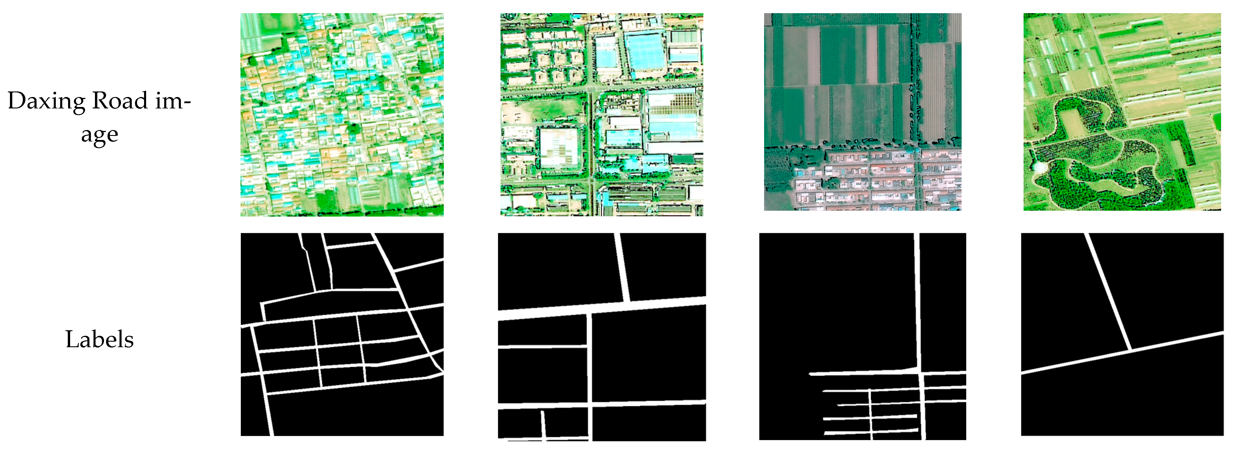
• The current deep models have better road extraction results in open-source datasets in HRSIs (e.g., DeepGlobe dataset [47], Massachusetts dataset [17], and SpaceNet dataset [48]). However, the robustness of the models has been tested only in fine-grained road extraction tasks [32,37,44]. Open-source datasets such as the DeepGlobe and the Massachusetts datasets, which are widely employed for remotely sensed road extraction [46,49], are less subject to external interference (e.g., vegetation cover, manual annotation). However, most of these datasets cover urban areas while ignoring the vast suburban zones [50]. Yao et al. demonstrate that models that perform well on open-source clear datasets have significantly lower road extraction capabilities in complex contexts, and road disturbances have not been learned enough [51]. As a matter of fact, most of the road areas in current HRSIs have problems such as high vegetation coverage, vague images, and large road spans, as shown in Figure 1, which will directly affect road extraction performance.
• The connectivity of the extracted roads in HRSIs is influenced by misinformation from the shadows of buildings and trees, the diversity of imaging conditions, and the spectral similarity of roads with other objects. This is one of the biggest challenges in road extraction [52]. Pixel-wise supervised learning models (e.g., patch-based DCNN, FCNs, DeconvNet, etc.) pay much attention to road extraction accuracy rather than the quality of road connectivity [10], leading to fragmented results. The GAN-based approaches show the advantage in maintaining road network connectivity; nevertheless, some studies suggest that these methods have no mechanism for constructing road network topology [37,53], and the symmetric encoder and decoder structure also contributes to feature redundancy and incorporates attritional noises into road connectivity judgment [36].
• Most current road extraction approaches from HRSIs focus on accuracy, efficiency, connectivity, and completeness [3,8,54], yet there is no metric that can describe the model’s lowest error boundary that can be achieved in the road extraction process, while the metric is extremely important for the evaluation of the robustness and universality of the specified model in practical applications [54]. Completeness, correctness, and quality are common standards to measure road extraction performance [15]. Pixel accuracy (PA) and mean pixel accuracy (mPA) are widely adopted to represent model effect in pixel-level accuracy. However, there is still a gap in the literature to measure the robustness and universality of deep learning models under the worst conditions in road extraction from HRSIs.

In this study, an asymmetric adversarial road extraction network (MS-AGAN) is proposed to tackle these problems mentioned above. The contributions of this study can be summarized as follows:

(1)

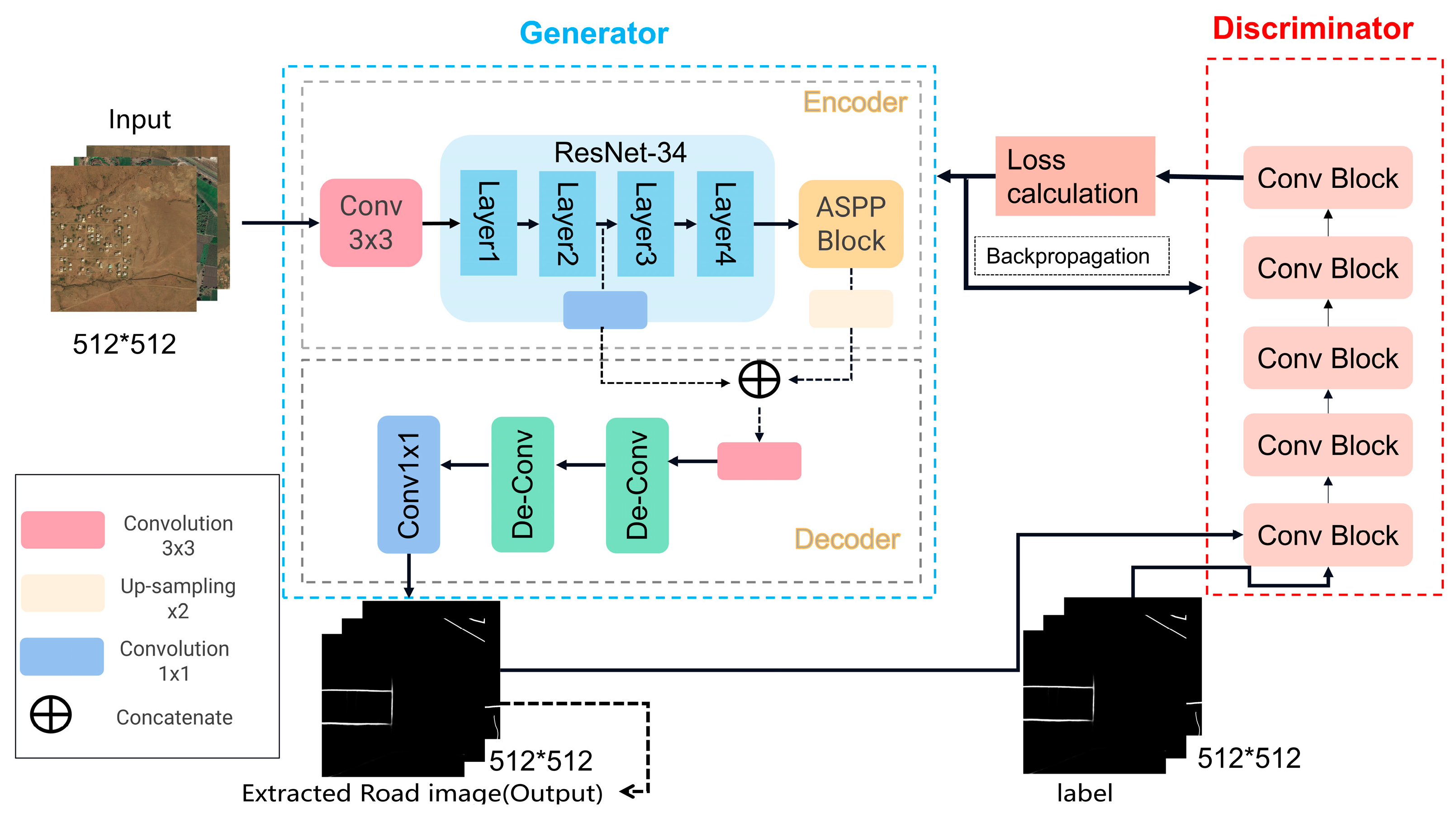
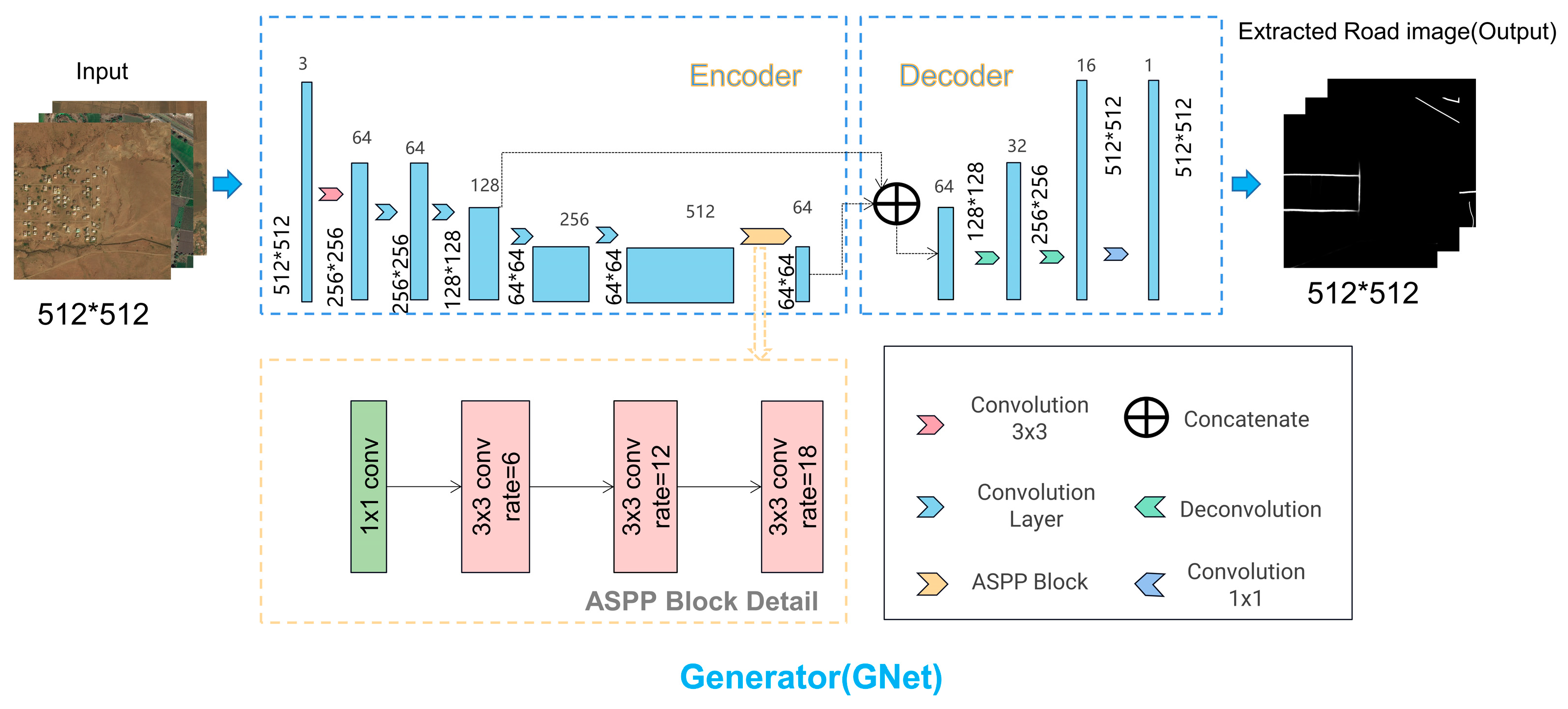
In MS-AGAN, we propose an asymmetric encoder–decoder generator to address the requirement for multi-scale road extraction in HRSIs. The enhanced encoder utilizes ResNet34 as the backbone network to extract high-dimensional features, while the simplified decoder eliminates the multi-scale cascading operations in symmetric structures to reduce the impact of noises. The ASPP and multi-scale feature fusion modules are integrated into the asymmetric encoder–decoder structure to avoid feature redundancy and to enhance the capability to extract fine-grained road information at the pixel level.

(2)

The topologic features are considered in the pixel segmentation process to maintain the connectivity of the road network. A linear structural similarity loss ($L_{SSIM}$) is introduced into the loss function of MS-AGAN, which guides MS-AGAN to generate more accurate segmentation results without auxiliary data or additional processing and to ensure that the extracted road information is more continuous and the model has stronger occlusion resistance.

(3)

Bayesian error rate (BER) is introduced into the field of road extraction to fairly evaluate the performance of deep models under complex backgrounds for the first time. BER determines the model’s lowest error boundary that can be achieved in road extraction from HRSIs, providing a practical metric for evaluating the universality and robustness of the models.

The remainder of this study is organized as follows. Section 2 briefly summarizes related works. Section 3 presents the details of MS-AGAN. Section 4 describes the dataset and experimental evaluation metrics and provides an experimental evaluation between MS-AGAN and current state-of-the-art methods, as well as an ablation study. Section 5 outlines the discussion and conclusions.

2. Related Works

2.1. Traditional Approaches for Road Extraction from HRSIs

Road extraction via remote sensing images traditionally relies heavily on prior knowledge of geometry, spectral characteristics, and background information of the roads. Road extraction methods that are based on morphological characteristics or manually designed features are the two main directions in traditional research [15].

Morphological features, including shapes, width, structures, etc., have a wide range of applications [55]. These features can be obtained through binarization, expansion, opening, and shutting [56,57,58,59]. In order to extract structural pixel information, Valero et al. introduce high-level directed morphological operators which include path openings and path closures in road extraction [60]. Chaudhuri et al. employ a semi-automatic method of road extraction that includes oriented morphological enhancement, oriented segmentation, and refinement [61]. Bae et al. introduce low-level and high-level processing methods for road extraction. Low-level and high-level processing methods identify the initial roads, which are then optimized locally with orientation and global graphical cuts [62]. These techniques often combine spectral and spatial features. However, it is still difficult to choose the best spectral or spatial features in various urban images [63]. Road forms can be effectively obtained from morphological feature-based approaches.

Following feature extraction, shallow models are employed with manually designed features. Typical shallow models include decision trees, support vector machines (SVM), Hough forests, tensor voting [64,65,66,67], etc. Movaghati et al. handle road extraction as a tracking problem by adopting manually designed features [68]. Wegner et al. extract road areas based on super-pixels. For each super-pixel feature representation, color and texture features are merged with 17-dimensional Gaussian filter bands [69]. To provide a more reliable road, Poullis et al. combine various feature extraction techniques, such as tensor coding and Gabor jets [70]. Maboudi et al. employ contextual feature integration strategies to extract road features. It contains tensor voting to categorize pixels as roads or backgrounds, and contextual feature integration strategies are applied to extract structural characteristics, spectral features, and text features [71]. Although road extraction methods based on manually designed features are typically more reliable than morphological-characteristic-based approaches, the low scalability across different data resources and parameter tuning still remains a big challenge [72,73,74].

2.2. Deep Learning Methods for Road Extraction from HRSIs

Road extraction techniques based on deep learning automatically build feature space from HRSIs [75]. The Legion model proposed by Yuan et al., which focuses on image segmentation, first extracts points on the inner axes of road segments to select potential road areas and then adopts group axis points within the road with aligned correlation connections [76]. Legion is considered as the initial work in neural-network-based road extractions. Subsequent deep-learning-based research mainly focuses on extraction accuracy and operation efficiency.

Deep-learning-based road extraction methods can be broadly classified into four genres [15], namely convolutional neural network (CNN) [2,77], full convolutional neural network (FCN) [28,78], U-shaped neural network (U-Net) [35,79], and generative adversarial network (GAN) [37,50].

Wei et al. propose a CNN-based model to extract road classes that provide road geometric information and spatial correlation, and then the model fuses deconvolution layers with the minimum Euclidean distance to generate a weighted mapping in road geometry [80]. A semi-automatic technique based on the finite-state machine (FSM) and deep neural networks (DNNs) is proposed by Wang et al. [81]. It consists of two parts: training and tracking. The training part defines a vector-guided tagging method based on vector road maps and images for direction matching. In the tracking phase, extracted image blocks are identified with a pre-trained DNN. This method shows good performance in general topography while behaving poorly under complicated circumstances (e.g., roads with a high vegetation coverage).

The FCN-based models apply additive operations to combine information from various layers [26]. These models abandon the final fully connected layer of the CNN. To guarantee the integrity and continuity of road networks, Zhang et al. derive an FCN-based model that is capable of extracting multi-spectral and terrain data [28]. In order to address the imbalance problem between road and background areas, Zhang et al. develop an FCN model with the weighting of the loss function among different road sections [82]. In order to extract road pixels, Chen et al. introduce a network called RVMNet which utilizes the FCN model for road node extraction and inserts road nodes into the road vector map [83].

In contrast to FCNs, U-Net-based models often apply cascading operations in feature fusion [84]. The encoder and decoder are the two main components in U-Net, which are often organized into a “U” form [85,86]. Li et al. propose Y-Net based on the U-Net architecture [87]. Y-Net has two modules for feature extraction and fusion. The fusion module in Y-Net merges features for road classification. However, the small road segments are often neglected in the Y-Net. By including a cascading dilated convolution module that extends the receptive field and extracts contextual information, Zhou et al. introduce D-LinkNet [44]. However, D-LinkNet still holds a high missing rate for narrow roads [7]. In order to improve the performance of road extraction, Xie et al. employ a higher-order spatial information global perception framework (HsgNet), which adopts LinkNet as the base network and embeds an intermediate block between the encoder and decoder [88]. This block learns to maintain various feature dependencies and channel information, distant spatial relationship information, and global contextual semantic information with smaller parameters than D-LinkNet. In order to improve the road topology, Ding et al. (2020) propose a direction-aware residual network (DiResNet). DiResNet contains two parts: the first is the structurally supervised asymmetric residual segmentation network (DiResSeg) which is designed for road topology learning, and the other is the refinement network (DiResRef) for fine-tuning segmentation [36]. Wan et al. suggest dense connections between neighboring convolutional layers and less pooling operations to preserve more road structure information [65]. He et al. integrate an encoder–decoder network with ASPP to collect multi-scale information, and they also introduce structural similarity metrics (SSIM) to the network training process [89]. Despite the fact that numerous studies have adopted U-Net-based models for road extraction [90,91], fragmentation under complex backgrounds still remains a major problem for multi-scale road extraction.

In recent studies, GAN-based models gradually attract attention in road extraction from HRSIs [37,38,50]. GAN consists of two parts: the generator and the discriminator. The generator of GAN generates additional samples from existing inputs, and the discriminator classifies the samples according to previous knowledge [15]. In the process of road extraction, the generator makes the generated images more realistic after the training procedure, and the discriminator becomes more powerful in differentiating real and generated samples [92]. The boundary information of road networks can be extracted more effectively according to GAN-based models regardless of occlusions and shadows [12], and the coverage of road networks becomes steadier [37]. Chen et al. propose an improved conditional generative adversarial network (NIGAN) [93]. In NIGAN, a road scene neighborhood confidence enhancement strategy is proposed to improve the connectivity of road extraction, and an improved ResNet34 and dilation convolution are incorporated to reduce the diameter of the road while preserving the main road features. NIGAN helps to extract better road features and prevent the overfitting problem. To reduce the reliance of deep models on large amounts of pixel-level annotated data, Chen et al. propose the semi-weakly generative adversarial network (SW-GAN), arguing that the OpenStreetMap (OSM) centerline can be considered as sparsely annotated labels [94]. SW-GAN requires only a small amount of precisely annotated data and a large amount of easily available weakly annotated data. However, OSM may have incomplete coverage and data errors, which directly affect practical applications [95]. Hu et al. propose an enhanced weakly supervised remote sensing image road network (WSGAN). WSGAN selects ResNet as the backbone network and employs the Patch GAN as GAN’S discriminator. It is believed that WSGAN can recover clearer mapped images in the occluded areas [96]. Zhang et al. propose the multi-supervised generative adversarial network (MsGAN), which focuses on the impact of occlusion and shadows on road extraction and learns how to reconstruct the occluded road based on the relationship between the visible road areas and the road centerlines [28]. Costea et al. propose a double-hop GAN (DH-GAN) network for extracting road topology. The combined DH-GAN and smoothing-based optimization (SBO) approach provides significant improvement in both topology and accuracy [97]. To overcome the cloud cover problem during road extraction, Rezaei et al. design an improved GAN network that combines an edge prediction framework with a color-filling component [98]. Pan et al. employ conditional generative adversarial networks (CGAN) and long- and short-term memory (LSTM) to build a semantic segmentation framework for high-resolution remote sensing images [99]. Zhang et al. adopt a deep convolutional generative adversarial network (DCGAN) for road extraction [38]. The generator in DCGAN relies on the FCN-based network. Similarly, Senthilnath et al. combine FCN and GAN to extract roads. Road areas are extracted via FCN, pix-2-pix, and CycleGAN, respectively, and the outputs are derived by voting strategy among different classifiers [4]. Shamsolmoali et al. design a GAN-based model containing a feature pyramid network (FP) module and introduce a new scale architecture to learn from multi-level feature mapping [50]. Shi et al. employ SeRNet to construct the generator part for road area extraction based on a novel end-to-end conditional GAN by optimizing the structural loss [100].

The GAN has a powerful feature shape prediction capability thanks to the adversarial training strategy, and its utilization for road extraction excels in terms of accuracy and is able to reduce the effects of building and tree occlusions [96]. However, current GAN-based models still lack mechanisms to construct road network topologies, thus limiting their practical application [53].

2.3. Road Connectivity

One of the important issues in road extraction is dealing with discontinuities and incompleteness in road features in high-resolution remote sensing images caused by a significant number of vehicles, buildings, and trees in complicated urban traffic and topographical situations [101]. At present, there are three different ways to deal with road connectivity: post-processing techniques based on the outcomes of road segmentation, multi-source data fusion techniques, and connectivity-processing techniques based on deep learning.

A number of post-processing techniques have been proposed for road connectivity reconstruction. These techniques include road geometry adoption [102], a marked point process [103], and integer programming on road graphs [104]. These methods take advantage of manually designed features. Mathematical morphology and Hough transform are also employed to connect small sections and discontinuous areas [105]. Richer convolutional features (RCFs) are applied in road segmentation and connection [106]. Non-road information is obliterated after the training process of the RCF network. However, the combination of pixels and the model structure in the post-processing phase neglects road width information.

Multi-source data fusion often refers to the communication among road centerlines, road areas, and related trajectories. Zhang et al. utilize a multi-supervised generative adversarial network to train the generator on both centerlines and road areas so as to recover the relationship between the road area and centerlines [37]. This method tends to behave more accurately for long, straight-road areas. Wei et al. extract road surface and centerlines simultaneously from remote sensing images via a multilevel-architecture-based CNN model [8] and fuse the rasterized centerline map with the segmentation of the road surface. The integration of road surface segmentation and road centerlines can relieve the discontinuities and incompleteness of road connectivity. However, complex backgrounds with high vegetation coverage and occlusions still remain a challenge. Gao et al. propose the DAD-LinkNet and introduce trajectories into the integration with roads extracted from heterogeneous remote sensing images [107]. Trajectories are considered as local semantic data which are adaptively combined with diverse road features with a self-attention mechanism.

Typical connectivity-processing techniques based on deep learning are designed to improve road network extraction capability and resolve occlusions and shadow-related disruptions. Zhou et al. propose a coarse-to-fine BT-RoadNet to predict coarse road segmentation maps and then bridge the discontinuities among road networks [3]. Chen et al. develop a road-scene neighborhood confidence enhancement strategy [93]. Structured loss functions are also employed to improve the completeness of road extraction [89,108]. Road connectivity is built with road skeletons as edges and road intersections as vertices [11,97,109]. However, the connectivity-processing techniques based on deep learning are sensitive to background information, and the efficiency is further influenced by the increase in data sources and data volumes [72].

2.4. Evaluation Metrics

Currently, the metrics, including quality, effectiveness, connectedness, and completeness, are frequently applied in road extraction from high-resolution images [15,110]. Correctness represents the percentage of the extracted road centerlines, which lies within the buffer around the reference network, whereas completeness is the percentage of the reference network that lies within the buffer around the extracted road centerlines, and quality considers both completeness and correctness [15]. Correctness, completeness, and quality in the remote sensing domain are often confused with the metrics of the confusion matrix in computer science. Completeness and correctness correspond to Recall and Precision, and the definition of quality is the same as IoU, the threat score (TS), the critical success index (CSI), or the Jaccard Index (JI) in the confusion matrix [111]. Pixel accuracy (PA) and mean pixel accuracy (mPA) are applied to determine the (average) percentage of correctly predicted pixels in each class. The topology metric (TOPO) is adopted to evaluate road network connectivity [11]. The shortest path (SP) is employed to measure how well the topology of the road network has been predicted [112]. However, the duplication of the SP is often challenged because the first two nodes in SP generation are randomly selected. The connected path ratio (CPR) incorporates the road segments in the SP metric and is calculated without interruptions [109]. To assess how comparable two graphs are to one another, Etten et al. employ the average path length similarity (APLS) [113]. Senthilnath et al. adopt the gap density (GD) to judge the fragmentation of the extracted outputs and calculate the average number of pixels occupied by each gap [4]. Abdollahi et al. present connectivity-preserving centerline Dice (CP_clDice) to quantify the shape and connectedness of roads [10]. To reflect the connectedness and topology of output in the local range, Wei Y. et al. employ the connectivity index, the ground reality center map is divided into segments of equal length, and the segments covered by the forecast segment map are treated as connecting roads [8].

The metrics mentioned above can reflect and evaluate the road extraction effect in various aspects, yet there is still no metric that can describe a model’s lowest error boundary that can be achieved in the road extraction process, which is extremely important to evaluate the model’s robustness in practical applications.

3. MS-AGAN Network

In this section, we first introduce the general framework of MS-AGAN, including the generator network GNet, the discriminator network DNet, and the hybrid loss function of the model. The structure of the proposed MS-AGAN is presented in Figure 2.

3.1. Generator GNet

The generator GNet is designed in the MS-AGAN to extract road features. GNet consists of two main components, including an enhanced encoder and a simplified decoder. The enhanced encoder consists of the improved ResNet34 and the ASPP module, passes through the original HRSI, and outputs the feature map with the spatial size of H/8*W/8, where H is the original image height, and W is the original image width. The improved ResNet34 produces multi-scale features, including lower-level features and high-level features. The low-level features are more closely related to the raw pixels of the image, and the high-level features are more robust and can be more helpful for tasks that require a higher level of understanding of the image contents. In addition, to better model the multi-scale features, the ASPP module is also added to the encoder to convolve a parallel sample with different sampling rates. The details of the ASPP module are described in Section 3.1.2.

The simplified decoder part of GNet integrates multi-scale features. Although it has been demonstrated that multi-scale cascading of low-level features in UNet-like architectures can improve the performance of road extraction [114,115,116], we argue that low-level features are usually noisier, and the skip connections between them may lead to uneven boundaries and disruptions. Hence, we replace the multi-scale cascading operations in UNet-like architectures with an asymmetric encoder–decoder structure in GNet so as to meet the requirement of multi-scale feature fusion. The final road prediction map is then constructed from GNet with the same size as the original image. Figure 3 shows the details of the GNet.

The enhanced encoder and simplified decoder can effectively preserve the high-dimensional features of roads and reduce the impact of environmental noise introduced with the multi-scale cascading operations. With the help of multi-scale feature fusion, low-dimensional features preserve the spatial boundaries of narrow roads, while high-level features embed the skeleton of the underlying road network. These designs enable the proposed network to better identify narrow roads in complex environments with high vegetation occlusion and large road width span.

3.1.1. Improved ResNet34

ResNet is commonly utilized as the backbone network in road extraction [117,118] because ResNet-based models can reduce redundant information while maintaining a fairly high convergence rate to avoid data collapse in deep networks [23,119,120,121]. In this study, ResNet34 [122] is employed as the backbone for road feature extraction. In order to better extract multi-scale features, the original ResNet34 architecture is modified as follows.

Firstly, the original ResNet34 contains 33 convolutional layers and 1 fully connected layer. In this study, ResNet34 only serves as the feature extractor, and hence the structure of ResNet34 is simplified: the fully connected layer in ResNet34 is removed, and the 7 × 7 convolutional kernel in the first layer is transferred to a 3 × 3 convolutional kernel. Afterward, to ensure that there are no duplicate areas between neighboring receptive fields in the 3 × 3 convolutional kernel and no information is missed, we set the step size in ResNet34 to 2, and the output matrix size is reduced to half of the input size. This “pooling” effect replaces the pooling layers in the original ResNet34 architecture. Thirdly, we employ stride operation in three convolutional blocks so as to enable the feature size to be gradually reduced. The details of the improved ResNet34 feature extractor are shown in Figure 4.

In Figure 4, in the improved ResNet34 network, after the convolution in the first layer, the network outputs a feature map with the size of (1/2H,1/2W,64). And the stride operation in the network is designed within the second, third, and fourth convolution blocks. In the first convolution block (layer1), the step size is set to 1, and the feature map goes through layer 1 with the same size. In layer 2, layer 3, and layer 4, the step sizes are all set to 2, and the feature map goes through layer 2, layer 3, and layer 4 with the size changing to (1/4H, 1/4W, 128), (1/8H, 1/8W, 256), and (1/8H, 1/8W, 512), respectively. Compared to the original ResNet which performs the stride operation only in one convolutional block, the stride operation in multiple convolutional blocks gradually tunes the feature map to a proper size.

3.1.2. The ASPP Module

In ResNet-like and FCN-based models, the overall receptive field grows slowly as the number of layers increases at the cost of information loss, the image size will be reduced, and the extraction result of the road will be interrupted or ignored. In this study, we introduce the ASPP module after layer4 (in Figure 4) to increase the perceptual field of the network without down-sampling and enhance the network’s ability to obtain multi-scale feature contexts. The ASPP module is shown in Figure 3, including one 1 × 1 convolution and three 3 × 3 atrous convolutions with the expansion rates of (6, 12, 18), respectively. And the feature map changes from the original (1/8H, 1/8W, 512) to (1/8H, 1/8W, 64) with the help of the ASPP module. For a given input, ASPP achieves parallel sampling with different sampling rates of atrous convolution, which in turn captures multi-scale contextual information and reduces information loss and thus guarantees road extraction performance at the process of generator network GNet.

3.1.3. Decoder Structure

In the decoder stage, we first fuse the output of layer2 with the output of ASPP for feature fusion. The output of layer 2 is composed of low-dimensional features which have high resolution with detailed location information, and the output of the ASPP module consists of high-dimensional features which may lose low-level details. The feature fusion process complements the detailed information missing from the high-dimensional features, as is shown in Figure 5.

Next, the second layer outputs the first part of the feature map via a 1 × 1 convolution, and the dimension changes from (H/4, W/4, 128) to (H/4, W/4, 64). The ASPP module also creates the second part of the feature map after the up-sampling strategy. The subsequent feature map is then concatenated with these two parts with the size of (H/4, W/4, 128).

Finally, to eliminate the overlap effect from the up-sampling process [91], the feature map is processed with a 3 × 3 convolution, and the final size of the feature map is (H/4, W/4, 64).

The feature fusion process between the output of layer2 and the output of ASPP (the last layer in the encoder part) allows for more road detail features and enhances the network’s ability to obtain multi-scale contextual features. After feature fusion, we introduce two deconvolution layers, which are employed to obtain a road prediction map of the same size as the original map. The decoding process is shown in the Decoder section in Figure 3. After the first layer deconvolution, the feature map with the size of (256, 256, 32) is created, and after the second layer deconvolution, the feature map of size (512, 512, 16) is regarded as the output. To ensure the final output channel equals one, the feature map of (512, 512, 16) is subjected to the 1 × 1 convolution operation. The final size of the prediction map is then (512, 512, 1).

3.2. Discriminator DNet

The road prediction map generated by GNet is still likely to contain interruptions and errors. The subsequent Discriminator in the proposed MS-AGAN is called DNet, which is designed to further refine the road prediction map at the post-processing stage. The Discriminator DNet is based on the FCN structure which can accept different input sizes. The architecture of DNet is shown in Figure 6.

In DNet, the prediction map generated by the generator is trained to make the network aware of the spectral structure, and a linear structure-supervised loss is added to guide the discriminator focusing on the topological connectivity during the adversarial learning process between GNet and DNet. The input of DNet includes the road prediction map from GNet and the ground truth labels. To ensure the channel number of the final outputs from DNet equals one, the DNet structure consists of five convolutional layers, and the size for each convolutional layer is equally set as $4\times 4$. The channel number in each convolutional layer is set as (64, 128, 256, 512, 1), respectively. After the process from five convolutional layers, the final confidence map with the size (H × W × 1) is then obtained via the Leaky-ReLU function.

Each pixel x in the confidence map is set to 1 if it is from a ground truth label and 0 if it is from a probability-like map. Adopting the confidence map approach, the prediction can be forced to split so that the parameters are spatially closer to the ground truth labels [123]. To enhance the connectivity of road extraction, a linear structural similarity loss is introduced into the DNet to calculate the structural similarity loss (SSIM) between the 1/8 result map of ground truth labels and the class probability-like map, guiding the GNet predictions to be more similar to the road structure in the labeled road networks.

3.3. Loss Function

In this study, to generate a more accurate and connected road network in MS-AGAN, we consider not only the pixel-level loss but also road topological loss to the original GAN loss function.

3.3.1. Generation Loss Function in GNet

The road extraction task in GNet can be regarded as a binary classification problem (i.e., “road” and “non-road”), and hence the binary cross-entropy loss function ($L_{BCE}$) is employed.

$$L_{BCE}=-\frac{1}{N}\sum _{n=1}^N\left({w_{1}y}_n\log \left(y_n^{\prime }\right)+w_0\left(1-y_n\right)\log \left(1-y_n^{\prime }\right)\right)$$

(1)

where $y_n$ is the ground truth of the n-th pixel, $y_n^{\prime }$ is the prediction of the n-th pixel, and N is the total number of the pixels.

However, the road area in HRSIs only accounts for a small part, and most of the image is the “non-road” area. If the same weight is given to the road and non-road areas in the loss function, the training process in the GNet of MS-AGAN will stop too early, and the accuracy of road extraction will be degraded. Therefore, a weighted hybrid loss function is proposed in GNet. The weight of the correctly labeled road areas is manually increased accordingly, and the penalty of false-negative labels is tuned higher than the false-positive labels according to [36].

$$L_{MSE}=\sum _{n=1}^N{(y_n-y_n^{\prime })}^2$$

(2)

$$L_G=L_{BCE}+{{\lambda }_{MSE}L}_{MSE}$$

(3)

where $L_G$, $L_{BCE}$, $L_{MSE}$ denote the loss of GNet, the loss of road area balance supervision, and the loss of road mean squared error supervision, respectively.

3.3.2. Discrimination Loss Function in DNet

The inputs to the Discriminator DNet are the road prediction map from GNet and the ground truth labels, and the output of DNet is the final confidence map with the size (H × W × 1). The value of a pixel in the confidence map indicates the likelihood of roads that are correctly classified. To train the DNet, the loss function is designed as follows.

$$L_D=-\frac{1}{N}\sum _{n=1}^N\left(z_n\log \left(D\left(I_n\right)\right)+\left(1-z_n\right)\log (1-D(G\left(X_n\right)\left)\right)\right)$$

(4)

where $X_n$ is the original image, $\mathrm{D}\left(\mathrm{G}\right({\mathrm{X}}_{\mathrm{n}}\left)\right)$ is the confidence map value of $X_n$ for the (h, w)th pixel, $I_n$ is the exterior product of the target label and the predicted label, $\mathrm{D}\left(I_n\right)$ is the confidence map value of $I_n$ for the (h, w)th pixel, $z_n=0$ if the discriminator’s input is $\mathrm{G}\left({\mathrm{X}}_{\mathrm{n}}\right)$, and $z_n=1$ if the discriminator’s input is $I_n$.

3.3.3. Topologic Structure Loss

The output confidence map in most traditional GAN-based models neglects the topological characteristics of road network structure. In this study, a linear structural similarity loss is adopted to construct road network connectivity. First, in order to focus on central road pixels, the ground truth map is down-sampled after area interpolation so as to narrow the road width. Then, the topological structure characteristic, that is, the spatial dependency between pixels, is introduced into the DNet. A linear structural similarity loss ($L_{SSIM}$) is introduced into the MS-AGAN’s loss function, as shown in Equation (5).

$$L_{SSIM}=1-SSIM\left(D\left(I_n\right),D\left(G\right(X_n\left)\right)\right)$$

(5)

where $SSIM\left(D\left(I_n\right),D\left(G\right(X_n\left)\right)\right)$ evaluates the similarity between two images by comparing luminance, contrast, and structure, $D\left(G\right(X_n\left)\right)$ is the confidence map value of $X_n$ for each pixel after down-sampling, and $D\left(I_n\right)$ is the confidence map value of $I_n$ for each pixel after down-sampling.

$SSIM\left(D\left(I_n\right),D\left(G\right(X_n\left)\right)\right)$ has three parts, where the first part of the luminance comparison function $l(p,q)$ compares the luminance by estimating the average intensity. Here, $p$ is $D\left(I_n\right),\mathrm{a}\mathrm{n}\mathrm{d} q$ is $D\left(G\right(X_n\left)\right)$. $l(p,q)$ is based on ${\mu }_p$ and ${\mu }_q$, defined by Equation (6).

$${\mu }_p=\frac{1}{n}\sum _{i=1}^N{p}_i$$

(6)

The second part of $SSIM\left(p,q\right)$ is the signal contrast, which is estimated by the standard deviation. The contrast function $c(p,q)$ is a function of ${\sigma }_p$ and ${\sigma }_q$. ${\sigma }_p$ is defined by Equation (7).

$${\sigma }_p={\left(\frac{1}{N-1}\sum _{i=1}^N{(p_i-{\mu }_p)}^2\right)}^{\frac{1}{2}}$$

(7)

The third part of $SSIM\left(p,q\right)$ is the structure comparison $s(p,q)$, which is estimated by correlation (inner product).$s(p,q)$ is composed of ${\sigma }_p$, ${\sigma }_q$, and ${\sigma }_{pq}$ and is defined by Equation (8).

$${\sigma }_{pq}=\frac{1}{N-1}\sum _{i=1}^N(p_i-{\mu }_p)(q_i-{\mu }_q)$$

(8)

The final representation is obtained by the three parts of $SSIM\left(p,q\right)$, which is defined by Equation (9). $p$ is $D\left(I_{nf}\right),\mathrm{a}\mathrm{n}\mathrm{d} q$ is $D\left(G\right(X_{nf}\left)\right)$.

$$SSIM\left(D\left(I_{nf}\right),D\left(G\right(X_{nf}\left)\right)\right)=\frac{(2{\mu }_p{\mu }_q+C_1)(2{\sigma }_{pq}+C_2)}{({{\mu }_p}^2+{{\mu }_q}^2+C_1)({{\sigma }_p}^2+{{\sigma }_q}^2+C_2)}$$

(9)

4. Experiments and Results

4.1. Datasets and Study Areas

Two datasets are selected for the experiments, including the GF-2 dataset of Daxing District, Beijing, and the DeepGlobe dataset [47]. Compared to most open-source datasets, the GF-2 dataset covers a variety of complex scenes with high vegetation cover and heavily obscured roads. The DeepGlobe dataset is a publicly available dataset adopted by many researchers.

4.1.1. DeepGlobe

This dataset is collected in Thailand, Indonesia, and India, covering a total area of approximately 2220 km², and the ground sampling distance (GSD) of the dataset is 50 cm per pixel. Each image has a size of 1024 × 1024 pixels. This dataset consists of 6226 training images, 1243 validation images, and 1101 test images. Since ground truth labels are only available in the training images, we select all training images as experimental data and randomly divide them into 4696 for training and 1530 for testing at a ratio of approximately 75%/25% according to the division criteria of previous studies [3,46]. This dataset is shown in Figure 7.

4.1.2. The GF-2 Dataset of Daxing District, Beijing

We manually annotate a GF-2 satellite imagery dataset of roads in Daxing District, Beijing, China. This dataset covers a total area of approximately 1100 km², and the ground sampling distance (GSD) of the dataset is 1 m per pixel. The images are cropped by 512 × 512 pixels, and a total of 5646 road images are obtained after the manual pre-processing. Following the same dataset partitioning criteria described in DeepGlobe, the training and test datasets are randomly partitioned at a ratio of 75%/25%, with 4209 images for training and 1437 images for testing. This dataset is shown in Figure 8.

4.2. Experimental Settings

All experiments are conducted on a workstation with 32 GB RAM and an NVIDIA Quadro P6000 GPU (16 GB).

The MS-AGAN is implemented with the PyTorch library [124]. The training batch size is set to 2. Since the experimental datasets have different GSDs, we choose different scaling rates for them in practical operations based on previous experience [36,125]. The minimum down-sampling rates for the dataset of Daxing District, Beijing, and the DeepGlobe dataset are 1/8 and 1/16, respectively. We utilize ResNet34 as the backbone network for the experiments on these two datasets. As road segmentation is a single-class segmentation problem that does not include complex modeling of semantic information, the number of layers in ResNet34 is sufficient to embed road features. The chosen down-sampling rate is implemented in all compared methods to ensure fairness.

4.3. Evaluation Metrics

In order to provide a comprehensive evaluation, six evaluation metrics are utilized, including Precision (P), Recall (R), F1 score, Intersection over Union (IoU), Bayesian error rate (BER), and connectivity (Conn). Recall and Precision [126] are the most common measurements in road extraction [17]. As road extraction can be regarded as a segmentation problem, road pixels are positive, and background pixels are negative. Therefore, all predictions can be categorized into the confusion matrix, including true positive (TP), true negative (TN), false positive (FP), and false negative (FN). True positive (TP) indicates that the road segments are detected correctly; true negative (TN) indicates that background pixels are correctly classified; false positive (FP) represents the ratio of misclassified road segments, and false negative (FN) denotes the ratio of misclassified non-road segments. All of these four metrics are defined (see (10)–(13)).

$$recall=\frac{TP}{TP+FN}$$

(10)

$$precision=\frac{TP}{TP+FP}$$

(11)

$$F1=\frac{2\times precision\times recall}{precision+recall}=\frac{2TP}{2TP+FN+FP}$$

(12)

$$IoU=\frac{TP}{TP+FP+FN}$$

(13)

We introduce the Bayesian error rate (BER) as a measure of the lowest classification error rate that can be achieved by a specified road extraction method. BER is a common evaluation metric in the medical field [127,128,129], indicating the lowest classification error rate that can be achieved by a specific model, and BER literally implies the effect of a model in the limit conditions of a known distribution [127,128,129]. The BER metric is defined in Equation (14).

$$\mathrm{B}\mathrm{E}\mathrm{R}=0.5\times (\frac{FN}{TP+FN}+\frac{FP}{FP+TN})$$

(14)

The connectivity (Conn) [8] is defined in Equation (15), which reflects the connectivity and topology of the road at a local scale. Specifically, the ground reality center map is divided into segments of equal length, and the segments covered by the prediction segment map are treated as connecting roads.

$$Conn=\frac{2N_{conn}}{N_{gt}+N_{pred}}$$

(15)

$N_{conn}$ is the number of connected segments, and $N_{gt}$ and $N_{pred}$ are the total numbers of segments on the ground reality center map and the prediction map, respectively.

Besides these quantitative evaluation metrics, we also qualitatively compare the performances among different models with visual comparisons.

4.4. Data Pre-Processing and Parameter Settings

The large amount of road data for road extraction is pre-processed as follows. First, the road vector map in the study area is downloaded from QuickOSM in QGIS and then transformed into a raster map. Second, the spatial coordinates in the raster map are written into GF-2 remote sensing images with ArcGIS so as to fulfill geographical alignment and semantic annotation. Finally, the aligned GF-2 remote sensing images and road vector map are cropped and manually sifted, and tiles with the size of 512 × 512 pixels are derived without overlap [130].

In this study, we compare MS-AGAN with typical methods in the literature, including RCFSNet [131], CoANet [46], UNet [43], DeepLabV3+ [45], and DiResNet [36]. RCFSNet combines road contextual information and full-stage feature fusion and performs well in occlusion scenes. CoANet shows better connectivity in extracted road networks via the DeepGlobe dataset. UNet and DeepLabV3+ have been widely applied and modified in road extraction from HRSIs. The architecture of DiResNet is similar to the GNet in MS-AGAN. Current GAN-based road extraction models (e.g., NIGAN [93], WSGAN [96], etc.) mainly focus on weakly supervised or unsupervised learning tasks. However, this study mainly focuses on supervised learning and employs the generative adversarial process to improve the performance and continuity of road extraction results. Due to the different purposes of algorithm designs, other GAN-based architectures are not selected as the baselines in this study. The training parameters for each method are summarized in

Table 1. Parameter settings of different models.

Model	Image Size	Learning Rate	Epoch	Batch Size
RCFSNet	512 × 512	0.01	150	2
CoANet	512 × 512	0.01	150	2
UNet	512 × 512	0.1	150	8
DeepLabV3+	512 × 512	0.1	150	8
DiResNet	512 × 512	0.1	150	8
MS-AGAN	512 × 512	0.001	150	2

.

4.5. Experimental Results and Evaluations

4.5.1. Performance Evaluation

Precision, Recall, F1-score, and IoU are selected for the evaluation of road extraction performance.

Table 2. Quantitative comparison on Daxing dataset (%). The bold represents the maximum value per column.

Model	Precision	Recall	F1	IoU
RCFSNet	61.54	62.87	58.72	43.09
CoANet	63.97	60.26	58.89	42.93
UNet	62.73	59.67	57.70	41.30
DeepLabV3+	62.92	62.15	59.47	43.33
DiResNet	65.34	59.88	59.08	42.76
MS-AGAN	61.05	65.04	59.51	45.96

reports the quantitative results of the compared methods with the GF-2 dataset.

As can be seen from Table 2, DiResNet achieves the best Precision with the help of its auxiliary supervision mechanism [36]. MS-AGAN achieves the best Recall (65.04%), F1(59.51%), and IoU (45.96%) because it preserves more shallow information in its network and fuses the lower-level features with the higher-level features to improve segmentation boundary accuracy. RCFSNet takes the second-best place in terms of the Recall (62.87%) metrics. DeepLabV3+ takes the second-best place in terms of the F1 (59.47%) and IoU (43.33%) metrics. Compared with RCFSNet, the Recall values of MS-AGAN on the Daxing dataset are 2.17% higher. Compared with DeepLabV3+, the F1 and IoU values of MS-AGAN on the Daxing dataset are 0.04% and 2.63% higher, respectively.

Table 3. Quantitative comparison on the DeepGlobe dataset (%). The bold represents the maximum value per column.

Model	Precision	Recall	F1	IoU
RCFSNet	75.90	77.34	74.83	62.09
CoANet	74.05	77.18	74.58	60.75
UNet	72.82	76.07	74.40	59.24
DeepLabV3+	76.97	76.18	74.61	62.03
DiResNet	79.92	73.99	74.75	62.39
MS-AGAN	75.66	78.46	75.25	62.64

reports the quantitative results of the DeepGlobe dataset. It can be seen that the designed MS-AGAN achieves the best results on Recall (78.46%), F1 (75.25%), and IoU (62.64%) because the addition of discriminators improves the continuity of spatial labels and refines the segmentation results. DiResNet achieves the best Precision (79.92%) and the second-best place in terms of F1 (74.75%) and IoU (62.39%) thanks to its supervised learning mechanism to enhance the embedding of road types and linear features. RCFSNet achieves the second-best place in terms of Recall (77.34%) and F1 (74.83%). Compared with DiResNet, the IoU values of MS-AGAN on the DeepGlobe dataset are 0.25% higher. Compared with RCFSNet, the Recall and F1 values of MS-AGAN on the DeepGlobe dataset are 1.12% and 0.42% higher, respectively.

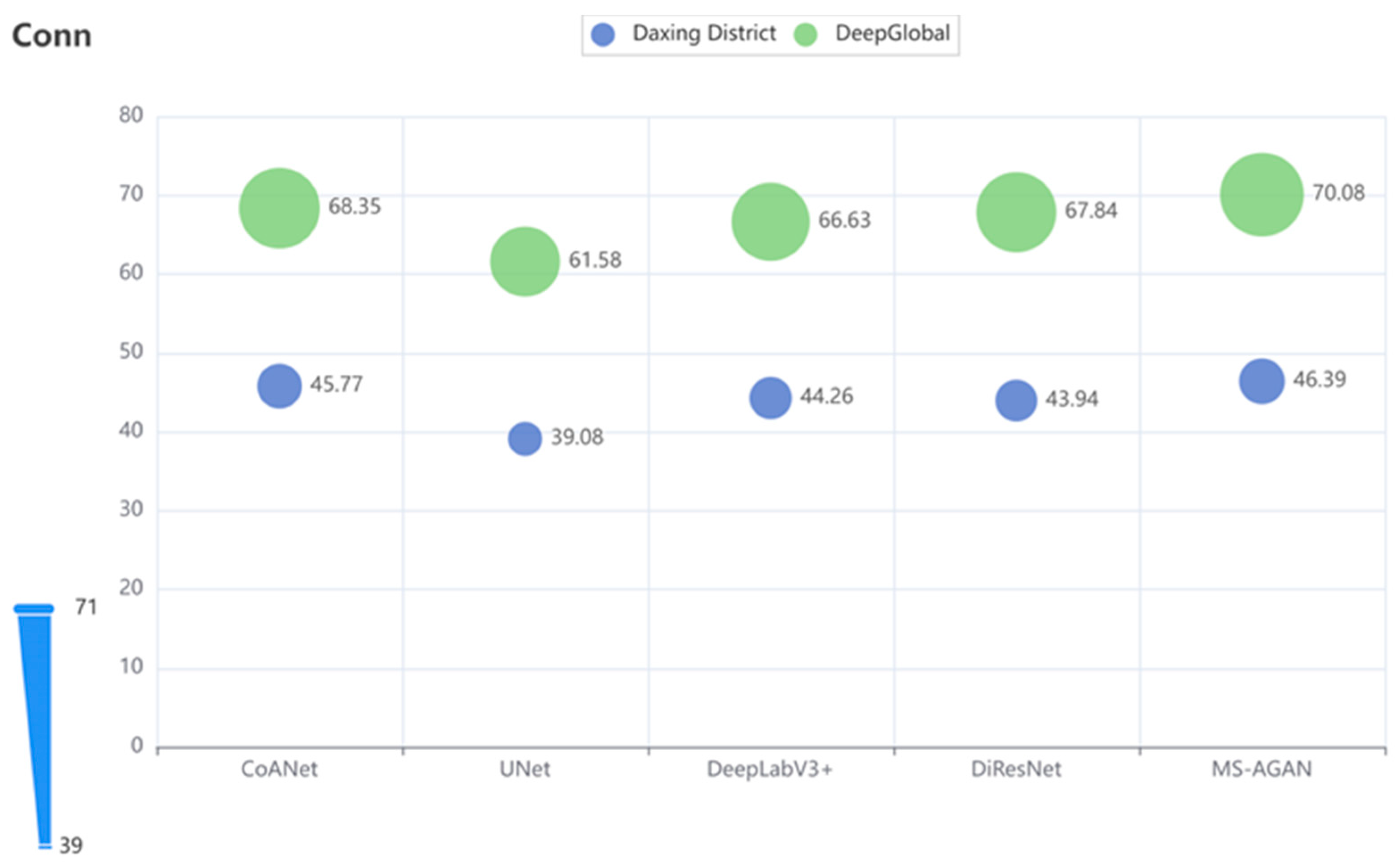
4.5.2. Evaluation of Road Connectivity

Figure 9 shows the quantitative connectivity evaluation for the comparison methods on the dataset of Daxing District, Beijing, and the DeepGlobe dataset, with the size of the circles in the figure representing the values of the connectivity scores.

As can be seen from Figure 9, MS-AGAN achieves the best connectivity scores on the Daxing (46.39%) and DeepGlobe (70.08%) datasets. CoANet takes the second-best connectivity scores on the Daxing (68.35%) and DeepGlobe (45.77%) datasets. Compared with CoANet, the designed MS-AGAN improves the connectivity scores by 0.62% on the dataset of Daxing District, Beijing, and 1.73% on the DeepGlobe dataset. Unlike CoANet, which only calculates the connectivity at the pixel level, the connectivity of MS-AGAN is mainly attributed to the introduction of topological structure supervision.

4.5.3. BER Evaluation

Figure 10 shows the quantitative results of Bayesian error rates comparing the methods on the dataset of Daxing District, Beijing, and the DeepGlobe dataset.

As can be seen from Figure 10, in terms of the new metric BER, MS-AGAN achieves the lowest BER scores both on the Daxing (20.86%) and DeepGlobe (11.77%) datasets. CoANet takes the second-lowest BER (21.08%) scores on the Daxing dataset. DeepLabV3+ takes the second-lowest BER (12.62%) scores on the DeepGlobe dataset. Compared with CoANet, MS-AGAN decreases the BER score by 0.22% on the dataset of Daxing District, Beijing. Compared with DeepLabV3+, MS-AGAN decreases the BER scores by 0.85% on the DeepGlobe dataset. These results show that the MS-AGAN has a lower Bayesian error rate, and the asymmetric generative adversarial structure of MS-AGAN plays a key role. On one hand, the asymmetric encoder and decoder structure effectively reduces the input of noisy information; on the other hand, the process of generating adversarial drives the prediction results of the generator to be more accurate. The lower Bayesian error rate demonstrates the robustness of MS-AGAN in practical applications.

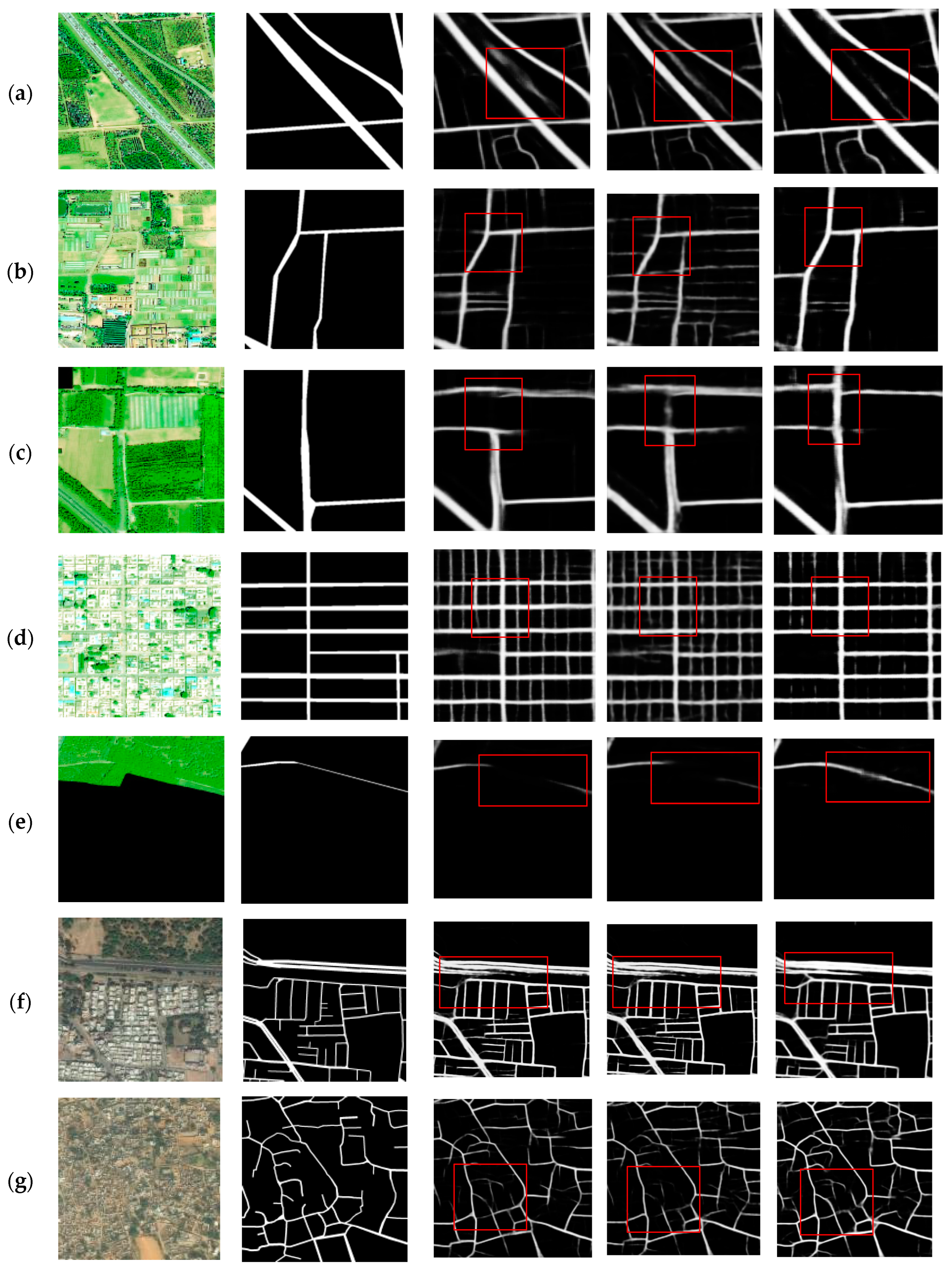
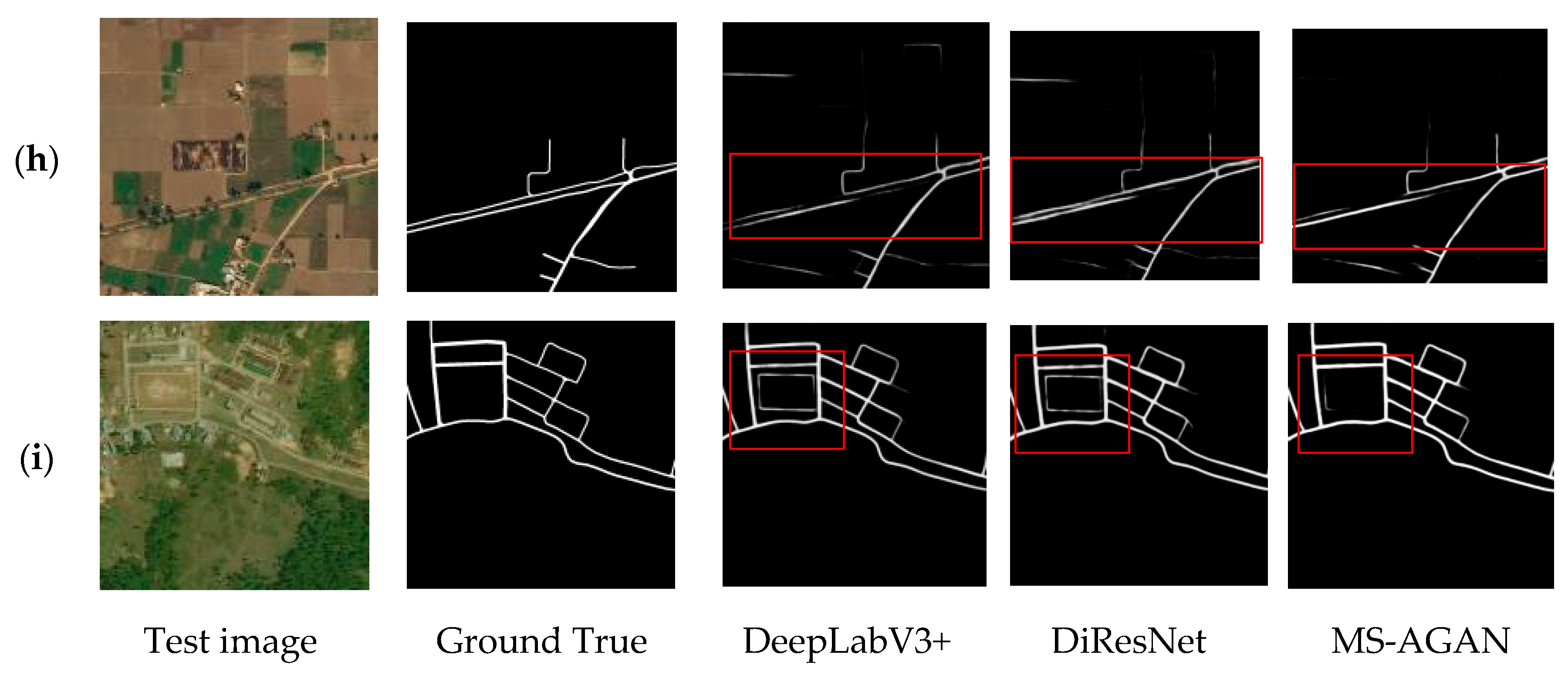
4.5.4. Qualitative Analysis

Following the quantitative analysis, we carry out a visual comparative analysis of the extraction results to explore the ability of the designed MS-AGAN on connectivity and road extraction.

Figure 11 shows an example of the qualitative results obtained through different methods. Figure 11a–e show the experimental results on the dataset of Daxing District in Beijing, China, and Figure 11f–i show the DeepGlobe dataset. Figure 11a shows a clearer example of the road area. Figure 11b shows examples of the presence of other features similar to the road feature. Figure 11c shows an example of a road area being obscured. Figure 11d shows an example of fine road extraction on a street scene. Figure 11e shows an example of a fine and obscured road area. The comparison shows that in areas with clear road images, the results from DiResNet and DeepLabV3+ are very close; MS-AGAN can extract clearer road boundaries with road widths than DiResNet and DeepLabV3+. In road areas with more complex backgrounds, DeepLabV3+ and DiResNet cannot distinguish other linear features from the road network and categorize them as roads, whereas MS-AGAN correctly categorizes road areas by gaining support from multi-scale feature information and removing low-level noises. Neither DiResNet nor DeepLabV3+ can extract roads from the occluded areas. MS-AGAN effectively extracts roads from the occluded areas by adding linear features to the discriminator, achieving better connectivity of roads. DiResNet and DeepLabV3+ also misidentify building boundary lines as roads when extracting street roads, while MS-AGAN is less disturbed by these features and produces fewer examples of errors. In fine-grained and occluded areas, DiResNet and DeepLabV3+ extract fragmented data, while MS-AGAN is still able to maintain connectivity with no breaks, and the extracted roads are clearer.

Figure 11f,g show the extraction results for street roads, while Figure 11h,i show the extraction results for country roads. For the extraction of street roads, our model suffers less from other linear interference and introduces less error information. For the extraction of country roads, MS-AGAN can better handle occlusions, and the introduction of linear features allows MS-AGAN to connect the breakpoints in the occluded areas. MS-AGAN shows better connectivity without causing more false alarms because other networks solve the connectivity by adding refinement networks, which introduce more low-level noises and cause more non-road features to be mistaken for road. We solve the connectivity problem by introducing road structure features and adopting GAN without introducing low-level noises. The accuracy of the road extraction results and the extraction of narrow roads are further guaranteed by the GAN structure. Compared to other methods, our proposed MS-AGAN shows two major advantages: (1) The addition of topological structure supervision improves the connectivity of extraction results and does not introduce low-level noises to interfere with outputs. (2) MS-AGAN produces more accurate road extraction results in complex scenes and can better distinguish road features from other linear features with fewer false alarms.

4.6. Ablation Study

This section analyzes the influence of hyperparameters and structural supervision in the modeling of MS-AGAN. For simplicity’s sake, all experiments in this section are conducted on the dataset of Daxing District, Beijing.

Table 4. Ablation results on the dataset of Daxing District, Beijing (%). The bold represents the maximum value per column.

Model	Sub-Nets		Module			Precision	Recall	F1
	Segmentation	Discriminator	Supervision	ASPP	CRF
ReNet	$\surd$					54.60	55.07	54.83
MS-AGAN_ASPP	$\surd$			$\surd$		56.41	55.13	55.76
GNet	$\surd$			$\surd$	$\surd$	59.88	55.25	57.47
MS-AGAN_S	$\surd$	$\surd$		$\surd$	$\surd$	60.95	59.47	60.20
MS-AGAN	$\surd$	$\surd$	$\surd$	$\surd$	$\surd$	61.05	65.04	62.98

reports the quantitative results of the ablation study on the dataset of Daxing District, Beijing. ReNet refers to the original asymmetric structured segmentation network without the discriminator part. MS-AGAN_ASPP refers to the ReNet that adds the ASPP module. GNet refers to the ReNet network that adds the ASPP and feature fusion module. MS-AGAN_S refers to the MS-AGAN model removing topological structure supervision. ReNet achieves the lowest place in terms of the Precision (54.60%), Recall (55.07%), and F1 (54.83%) metrics. Compared with ReNet, MS-AGAN_ASPP shows 1.81%, 0.06%, and 0.93% increases in Precision, Recall, and F1 because the ASPP module significantly improves the accuracy of the extraction results. Compared with MS-AGAN_ASPP, GNet with the fusion of the low-level features and high-level features achieves a 3.47% increase in Precision, a 0.12% increase in Recall, and a 1.71% increase in F1; the model obtains more information from the low-level layer, and the performance of extraction results becomes better. However, the rise in Recall is slow, mainly due to much occlusion in the image. The inclusion of multi-scale features can effectively solve the accuracy problem, so that small targets in the low-level layers have more information and improve the accuracy, but they are not effectively extracted in occluded roads. Compared to GNet, the inclusion of the discriminator in MS-AGAN_S increases Precision by 1.07%, Recall by 4.22%, and F1 by 2.73%, mainly because the GAN structure is effective in improving the connectivity of the extraction results and smoothing the results by concatenating the breakpoints. Compared to MS-AGAN_S, the addition of structural supervision in MS-AGAN increases Precision by 0.1%, Recall by 5.57%, and F1 by 2.78%, which is a significant increase in Recall. The addition of linear features also makes the road extraction results more coherent.

Figure 12 shows a comparison of results in the case of the generator with and without adding the discriminator. Figure 12a,b show the extraction results for areas with streets and heavily obscured roads.

It can be seen that the discriminator is added so that more streets are extracted and the road boundaries are clearer. Compared to GNet, MS-AGAN connects the fragmented road segments, and it can be seen that the extraction results are more connected. Figure 12c,d show the results of road extraction in areas with other linear features interfering. GNet’s extraction results have more fragmented roads and noise, other linear features barely interfere with MS-AGAN, and the extraction results are almost identical to the ground truth labels. In summary, the addition of the discriminator effectively improves the connectivity of the road extraction results, enabling fragmented roads to be connected, with clearer road boundaries and less interference from other linear features, effectively enhancing the accuracy of the network in extracting fine-grained roads.

Table 5. Comparison of different weight settings between the generator loss function and the linear structural similarity loss function (%). The bold represents the maximum value per column.

ID	Loss	Precision	Recall	F1	IoU
1	0.3$L_D$ + 0.7$L_{SSIM}$	56.47	64.36	60.15	43.01
2	0.5$L_D$ + 0.5$L_{SSIM}$	61.05	65.04	62.98	45.96
3	0.7$L_D$ + 0.3$L_{SSIM}$	61.13	61.30	61.21	44.10

reports the effect of the weight setting of the hybrid loss function in the discriminator on the results. The first column of Table 5 shows the experiment IDs for different parameter settings. In experiment 1, the linear structural similarity loss between the generator prediction graph and the labeled result graph is given greater weight. In experiment 2, the same weight is given. In experiment 3, the loss ($L_D$) of the discriminator judgments of truth and falsity is given greater weight.

Experiment 1 achieves the lowest place in terms of the Precision (56.47%), Recall (64.36%), F1 (60.15%), and IoU (43.01%) metrics. Compared to experiment 1, the increased weight of $L_D$ in experiment 2 improves Precision by 4.58%, Recall by 0.68%, F1 by 2.83%, and IoU by 2.95%. The increased output loss weight of the discriminator is significant in improving road extraction performance. We then try to continue to increase the discriminator output loss weights and decrease the structural loss weights. Compared with experiment 2, Precision increases by 0.08% in experiment 3, while Recall decreases by 3.74%, F1 decreases by 1.77%, and IoU decreases by 1.86%. Although the increase in discriminator output loss is effective in improving accuracy, the reduction in structural loss weight significantly affects the recall result. The inclusion of structural losses is effective to obtain more road information.

Table 6. Comparison of different weight settings of the generator loss function (%). The bold represents the maximum value per column.

ID	Loss	Precision	Recall	F1	IoU
1	$L_{BCE}$ + 0.7$L_{MSE}$	56.22	59.59	57.85	40.70
2	$L_{BCE}$ + 0.5$L_{MSE}$	61.05	65.04	62.98	45.96
3	$L_{BCE}$ + 0.3$L_{MSE}$	57.05	66.78	61.53	44.43

reports the effect of the weight setting of the hybrid loss function in the generator on the results. The first column of Table 6 shows the experiment IDs for different parameter settings. In experiment 1, the loss of road mean squared error supervision ($L_{MSE}$) is given a larger weight. In experiment 2, the weight of 0.5 is chosen. In experiment 3, $L_{MSE}$ is set with a smaller weight. Experiment 1 achieves the lowest Precision (56.22%), Recall (59.59%), F1 (57.85%), and IoU (40.70%) metrics. Compared to experiment 1, the decreased weight of $L_{MSE}$ in experiment 2 improves Precision, Recall, F1, and IoU by 4.83%, 5.45%, 5.13%, and 5.26%, respectively. The decreased weight of $L_{MSE}$ is significant in improving road extraction performance. We then try to continue to decrease the weight of $L_{MSE}$. Compared with experiment 2, Recall increases by 1.74% in experiment 3, while Precision decreases by 4%, F1 decreases by 1.45%, and IoU decreases by 1.53%. Although the decrease in $L_{MSE}$ is effective in improving Recall, it also significantly affects the Precision result.

The ablation study demonstrates that the ASPP module and multi-scale feature fusion in MS-AGAN can effectively solve the information loss problem during multiple down-sampling processes, and the inclusion of multi-scale features significantly improves the performance. Compared with the single extraction network GNet, the adoption of GAN can effectively improve the connectivity of the extraction results and repair the missing parts of the road. Topologic structure supervision introduces linear features to further discover obscured roads and repair broken roads, making the road extraction results more connected.

4.7. Time Complexity Studies

Training time, inference speed, parameters, and FLOPS are selected for the complexity analysis experiment. Training time is the average time required to train an epoch with the same dataset. Inference speed is the time to make predictions on the same dataset. The floating point operations per second (FLOPS) are calculated based on an input size of (3, 512, 512). All experiments are performed on the same equipment.

As can be seen from

Table 7. Time complexity studies of different methods on the Daxing dataset.

Model	Training Time (s)	Inference Speed (s)	Parameters (M)	FLOPS (Gps)
RCFSNet	589.00	73.79	59.278	207.816
CoANet	673.44	67.32	59.147	277.416
UNet	208.50	18.07	9.16	221.43
DeepLabV3+	331.60	62.15	22.704	100.538
DiResNet	397.30	59.88	21.321	115.473
MS-AGAN	950.16	98.44	25.114	126.08

, DeepLabV3+ takes the least FLOPS. The number of parameters in UNet is the smallest. UNet has the lowest training time and inference speed. Compared to the baseline method, MS-AGAN has no significant consumption on parameters and FLOPS. However, its training time and reasoning speed consumption becomes larger. We speculate that this is mainly related to its network structure.

5. Discussion and Conclusions

5.1. Discussion

As described in the experiments above, the proposed MS-AGAN achieves optimal performance on both the dataset of Daxing District, Beijing, and the open-source DeepGlobe dataset. However, MS-AGAN still has some failure cases. As shown in Figure 13a, for areas that are completely obscured by trees at intersections, although MS-AGAN can extract all road links, the road links cannot connect well to the second intersection. These areas are uniformly shown as trees on the satellite map. As shown in Figure 13b, in the area where the urban–rural junction is also obscured by trees, all models ignore the extraction of this minor road. As shown in Figure 11h, for rural fine-grained roads that are shaded, the roads in these areas may not be visible in the satellite images because the roads are too slender, and also the road areas are seriously affected by shaded occlusion. Although MS-AGAN performs better than other models, there are still inevitable breakpoints and shortcomings. In the future, we will consider road networks as graphs with edges and nodes and try to use graph convolutional networks to further improve road extraction performance in such areas.

In the ablation experiments, we discuss the effect of different weights of loss function on the road extraction performance and choose the weights corresponding to the optimal result in this network. However, in this experiment, there are other parameter settings that can affect the exaction results, such as the choice of convolutional kernels and step size, etc. Different choices of convolutional kernels and different step size settings will also have an impact on the extraction performance. In this study, we only employ the current common convolutional kernel with the setting of $3\times 3$ and do not analyze other convolutional kernel sizes. In addition, it can be seen in Table 7 that our model still has room for improvement in terms of training time and inference speed. How to choose lightweight models to achieve optimal extraction in a shorter time is also an issue we need to solve in the future.

5.2. Conclusions and Future Directions

Road extraction from HRSIs is an important direction in remote sensing analysis. The fragmentation of extraction results and the inability to balance the extraction of complex scenes with narrow roads are the key problems in road extraction from HRSIs.

In this study, we propose an asymmetric adversarial learning network (MS-AGAN) model to extract multi-scale roads from high-resolution remote sensing images. First, the MS-AGAN’s generator adopts an asymmetric encoder–decoder structure for road pixel extraction, and the enhanced encoder utilizes ResNet34 as the backbone network to extract high-dimensional features and adds fusion of atrous convolution and low-dimensional features in the last layer to enhance the network’s ability to obtain small-scale contextual information. The simplified decoder removes the multi-level cascade operation in the symmetric structure to reduce the input of noisy information, and the step-by-step deconvolution process retains more high-dimensional information compared to the original FCN. Second, the MS-AGAN’s discriminator employs the FCN-based architecture, and for the task of road extraction with high vegetation cover, we enhance the original GAN loss function by adding a linear structure-based loss term as topological structural supervision to ensure that the extracted road information is more connected, and the model is more resistant to occlusion. Unlike most methods based on road centerline and edge detection, we effectively guide the training process of the generator by adding topological structural supervision to the discriminator, thus solving the road extraction connectivity problem without additional training. Finally, to fairly evaluate the performance of deep models under complex backgrounds, the Bayesian error rate (BER) is introduced into the field of road extraction for the first time.

The experimental results show that the proposed MS-AGAN is able to handle interruptions caused by shadows and occlusions, extract roads of different widths and materials, and tackle roads with incomplete spectral and geometric features. The proposed MS-AGAN provides an efficient, cost-effective, and reliable method for the dynamic updating of road networks via HRSIs. Compared with available road extraction methods, the connectivity of the extracted road network from MS-AGAN is better, and the architecture is much simpler for practical application.

In the future, we will continue to apply other neural network architectures for road extraction. To extend the application of road extraction models, transfer learning methods will be investigated to improve the generalization ability of road extraction methods.

References

1. Bakhtiari, H.R.R.; Abdollahi, A.; Rezaeian, H. Semi automatic road extraction from digital images. Egypt. J. Remote Sens. Space Sci. 2017, 20, 117–123. [Google Scholar] [CrossRef]
2. Liu, P.; Di, L.; Du, Q.; Wang, L. Remote sensing big data: Theory, methods and applications. Remote Sens. 2018, 10, 711. [Google Scholar] [CrossRef] [Green Version]
3. Zhou, M.; Sui, H.; Chen, S.; Wang, J.; Chen, X. BT-RoadNet: A boundary and topologically-aware neural network for road extraction from high-resolution remote sensing imagery. ISPRS J. Photogramm. Remote Sens. 2020, 168, 288–306. [Google Scholar] [CrossRef]
4. Senthilnath, J.; Varia, N.; Dokania, A.; Anand, G.; Benediktsson, J.A. Deep tec: Deep transfer learning with ensemble classifier for road extraction from Uav imagery. Remote Sens. 2020, 12, 245. [Google Scholar] [CrossRef] [Green Version]
5. Tan, Y.Q.; Gao, S.H.; Li, X.Y.; Cheng, M.M.; Ren, B. Vecroad: Point-based iterative graph exploration for road graphs extraction. In Proceedings of the IEEE/CVF Conference on Computer Vision and Pattern Recognition, Seattle, WA, USA, 13–19 June 2020; pp. 8910–8918. [Google Scholar]
6. Abdollahi, A.; Pradhan, B.; Alamri, A. VNet: An end-to-end fully convolutional neural network for road extraction from high-resolution remote sensing data. IEEE Access 2020, 8, 179424–179436. [Google Scholar] [CrossRef]
7. Wang, Y.; Seo, J.; Jeon, T. NL-LinkNet: Toward lighter but more accurate road extraction with nonlocal operations. IEEE Geosci. Remote Sens. Lett. 2021, 19, 1–5. [Google Scholar] [CrossRef]
8. Wei, Y.; Zhang, K.; Ji, S. Simultaneous Road Surface and Centerline Extraction From Large-Scale Remote Sensing Images Using CNN-Based Segmentation and Tracing. IEEE Trans. Geosci. Remote Sens. 2020, 58, 8919–8931. [Google Scholar] [CrossRef]
9. Panteras, G.; Cervone, G. Enhancing the temporal resolution of satellite-based flood extent generation using crowdsourced data for disaster monitoring. Int. J. Remote Sens. 2018, 39, 1459–1474. [Google Scholar] [CrossRef]
10. Abdollahi, A.; Pradhan, B.; Alamri, A. SC-RoadDeepNet: A New Shape and Connectivity-Preserving Road Extraction Deep Learning-Based Network from Remote Sensing Data. IEEE Trans. Geosci. Remote Sens. 2022, 60, 1–15. [Google Scholar] [CrossRef]
11. Bastani, F.; He, S.; Abbar, S.; Alizadeh, M.; Balakrishnan, H.; Chawla, S.; DeWitt, D. Roadtracer: Automatic extraction of road networks from aerial images. In Proceedings of the IEEE Conference on Computer Vision and Pattern Recognition, Salt Lake City, UT, USA, 18–23 June 2018; pp. 4720–4728. [Google Scholar]
12. Abdollahi, A.; Pradhan, B.; Shukla, N.; Chakraborty, S.; Alamri, A. Deep learning approaches applied to remote sensing datasets for road extraction: A state-of-the-art review. Remote Sens. 2020, 12, 1444. [Google Scholar] [CrossRef]
13. Ma, Y.; Wu, H.; Wang, L.; Huang, B.; Ranjan, R.; Zomaya, A.; Jie, W. Remote sensing big data computing: Challenges and opportunities. Future Gener. Comput. Syst. 2015, 51, 47–60. [Google Scholar] [CrossRef] [Green Version]
14. Abdollahi, A.; Pradhan, B.; Alamri, A. RoadVecNet: A new approach for simultaneous road network segmentation and vectorization from aerial and google earth imagery in a complex urban set-up. GIScience Remote Sens. 2021, 58, 1151–1174. [Google Scholar] [CrossRef]
15. Chen, Z.; Deng, L.; Luo, Y.; Li, D.; Junior, J.M.; Gonçalves, W.N.; Li, D. Road extraction in remote sensing data: A survey. Int. J. Appl. Earth Obs. Geoinf. 2022, 112, 102833. [Google Scholar] [CrossRef]
16. Mnih, V.; Hinton, G.E. Learning to detect roads in high-resolution aerial images. In Computer Vision—ECCV 2010; Daniilidis, K., Maragos, P., Paragios, N., Eds.; Lecture Notes in Computer Science; Springer: Berlin/Heidelberg, Germany, 2010; Volume 6316. [Google Scholar] [CrossRef]
17. Mnih, V. Machine Learning for Aerial Image Labeling. Ph.D. Thesis, University of Toronto, Toronto, ON, Canada, 2013. [Google Scholar]
18. Amit, S.N.K.B.; Aoki, Y. Disaster detection from aerial imagery with convolutional neural network. In Proceedings of the 2017 International Electronics Symposium on Knowledge Creation and Intelligent Computing (IES-KCIC), Surabaya, Indonesia, 26–27 September 2017; IEEE: New York, NY, USA, 2017; pp. 239–245. [Google Scholar]
19. Pi, Y.; Nath, N.D.; Behzadan, A.H. Convolutional neural networks for object detection in aerial imagery for disaster response and recovery. Adv. Eng.Inform. 2020, 43, 101009. [Google Scholar] [CrossRef]
20. Atwood, J.; Towsley, D. Diffusion-convolutional neural networks. Adv. Neural Inf. Process. Syst. 2016, 29, 2001–2009. [Google Scholar]
21. Simonyan, K.; Zisserman, A. Very deep convolutional networks for large-scale image recognition. arXiv 2014, arXiv:1409.1556. [Google Scholar]
22. He, K.; Zhang, X.; Ren, S.; Sun, J. Deep residual learning for image recognition. In Proceedings of the IEEE Conference on Computer Vision and Pattern Recognition, Las Vegas, NV, USA, 26 June–1 July 2016; pp. 770–778. [Google Scholar]
23. Szegedy, C.; Ioffe, S.; Vanhoucke, V.; Alemi, A. Inception-v4, inception-resnet and the impact of residual connections on learning. In Proceedings of the Thirty-First AAAI Conference on Artificial Intelligence, San Francisco, CA, USA, 4–9 February 2017. [Google Scholar]
24. Howard, A.G.; Zhu, M.; Chen, B.; Kalenichenko, D.; Wang, W.; Weyand, T.; Adam, H. Mobilenets: Efficient convolutional neural networks for mobile vision applications. arXiv 2017, arXiv:1704.04861. [Google Scholar]
25. Chen, L.; Zhu, Q.; Xie, X.; Hu, H.; Zeng, H. Road extraction from VHR remote-sensing imagery via object segmentation constrained by Gabor features. ISPRS Int. J. Geo-Inf. 2018, 7, 362. [Google Scholar] [CrossRef] [Green Version]
26. Long, J.; Shelhamer, E.; Darrell, T. Fully convolutional networks for semantic segmentation. In Proceedings of the IEEE Conference on Computer Vision and Pattern Recognition, Boston, MA, USA, 8–10 June 2015; pp. 3431–3440. [Google Scholar]
27. Patil, D.; Jadhav, S. Road extraction techniques from remote sensing images: A review. In Innovative Data Communication Technologies and Application, Proceedings of ICIDCA 2020, Coimbatore, India, 3–4 September 2020; Springer: Berlin/Heidelberg, Germany, 2021; pp. 663–677. [Google Scholar]
28. Zhang, Y.; Xia, G.; Wang, J.; Lha, D. A multiple feature fully convolutional network for road extraction from high-resolution remote sensing image over mountainous areas. IEEE Geosci. Remote Sens. Lett. 2019, 16, 1600–1604. [Google Scholar] [CrossRef]
29. Pan, D.; Zhang, M.; Zhang, B. A generic FCN-based approach for the road-network extraction from VHR remote sensing images–using openstreetmap as benchmarks. IEEE J. Sel. Top. Appl. Earth Obs. Remote Sens. 2021, 14, 2662–2673. [Google Scholar] [CrossRef]
30. Xu, Z.; Shen, Z.; Li, Y.; Xia, L.; Wang, H.; Li, S.; Jiao, S.; Lei, Y. Road extraction in mountainous regions from high-resolution images based on DSDNet and terrain optimization. Remote Sens. 2020, 13, 90. [Google Scholar] [CrossRef]
31. Ge, Z.; Zhao, Y.; Wang, J.; Wang, D.; Si, Q. Deep feature-review transmit network of contour-enhanced road extraction from remote sensing images. IEEE Geosci. Remote Sens. Lett. 2021, 19, 1–5. [Google Scholar] [CrossRef]
32. Zou, W.; Feng, D. Multi-dimensional attention unet with variable size convolution group for road segmentation in remote sensing imagery. In Proceedings of the 2022 2nd Asia-Pacific Conference on Communications Technology and Computer Science (ACCTCS), Shenyang, China, 25–27 February 2022; IEEE: New York, NY, USA, 2022; pp. 328–334. [Google Scholar]
33. Chen, G.; Li, C.; Wei, W.; Jing, W.; Woźniak, M.; Blažauskas, T.; Damaševičius, R. Fully Convolutional Neural Network with Augmented Atrous Spatial Pyramid Pool and Fully Connected Fusion Path for High Resolution Remote Sensing Image Segmentation. Appl. Sci. 2019, 9, 1816. [Google Scholar] [CrossRef] [Green Version]
34. Liu, Y.; Yao, J.; Lu, X.; Xia, M.; Wang, X.; Liu, Y. Roadnet: Learning to comprehensively analyze road networks in complex urban scenes from high-resolution remotely sensed images. IEEE Trans. Geosci. Remote Sens. 2018, 57, 2043–2056. [Google Scholar] [CrossRef]
35. Wang, S.; Mu, X.; Yang, D.; He, H.; Zhao, P. Road extraction from remote sensing images using the inner convolution integrated encoder-decoder network and directional conditional random fields. Remote Sens. 2021, 13, 465. [Google Scholar] [CrossRef]
36. Ding, L.; Bruzzone, L. DiResNet: Direction-aware residual network for road extraction in VHR remote sensing images. IEEE Trans. Geosci. Remote Sens. 2020, 59, 10243–10254. [Google Scholar] [CrossRef]
37. Zhang, Y.; Xiong, Z.; Zang, Y.; Wang, C.; Li, J.; Li, X. Topology-aware road network extraction via multi-supervised generative adversarial networks. Remote Sens. 2019, 11, 1017. [Google Scholar] [CrossRef] [Green Version]
38. Zhang, X.; Han, X.; Li, C.; Tang, X.; Zhou, H.; Jiao, L. Aerial Image Road Extraction Based on an Improved Generative Adversarial Network. Remote Sens. 2019, 11, 930. [Google Scholar] [CrossRef] [Green Version]
39. Batra, A.; Singh, S.; Pang, G.; Basu, S.; Jawahar, C.V.; Paluri, M. Improved road connectivity by joint learning of orientation and segmentation. In Proceedings of the IEEE/CVF Conference on Computer Vision and Pattern Recognition, Long Beach, CA, USA, 15–20 June 2019; pp. 10385–10393. [Google Scholar]
40. Varia, N.; Dokania, A.; Senthilnath, J. DeepExt: A convolution neural network for road extraction using RGB images captured by UAV. In Proceedings of the 2018 IEEE Symposium Series on Computational Intelligence (SSCI), Bangalore, India, 18–21 November 2018; IEEE: New York, NY, USA, 2018; pp. 1890–1895. [Google Scholar]
41. Yang, C.; Wang, Z. An ensemble Wasserstein generative adversarial network method for road extraction from high resolution remote sensing images in rural areas. IEEE Access 2020, 8, 174317–174324. [Google Scholar] [CrossRef]
42. Chen, H.; Li, Z.; Wu, J.; Xiong, W.; Du, C. SemiRoadExNet: A semi-supervised network for road extraction from remote sensing imagery via adversarial learning. ISPRS J. Photogramm. Remote Sens. 2023, 198, 169–183. [Google Scholar] [CrossRef]
43. Ronneberger, O.; Fischer, P.; Brox, T. U-net: Convolutional networks for biomedical image segmentation. In Medical Image Computing and Computer-Assisted Intervention, Proceedings of the MICCAI 2015 18th International Conference, Munich, Germany, 5–9 October 2015; Part III 18; Springer International Publishing: Cham, Switzerland, 2015; pp. 234–241. [Google Scholar]
44. Zhou, L.; Zhang, C.; Wu, M. D-LinkNet: LinkNet with pretrained encoder and dilated convolution for high resolution satellite imagery road extraction. In Proceedings of the IEEE Conference on Computer Vision and Pattern Recognition Workshops, Salt Lake City, UT, USA, 18–22 June 2018; pp. 182–186. [Google Scholar]
45. Chen, L.C.; Papandreou, G.; Kokkinos, I.; Murphy, K.; Yuille, A.L. Deeplab: Semantic image segmentation with deep convolutional nets, atrous convolution, and fully connected crfs. IEEE Trans. Pattern Anal. Mach. Intell. 2017, 40, 834–848. [Google Scholar] [CrossRef] [PubMed] [Green Version]
46. Mei, J.; Li, R.J.; Gao, W.; Cheng, M.M. CoANet: Connectivity attention network for road extraction from satellite imagery. IEEE Trans. Image Process. 2021, 30, 8540–8552. [Google Scholar] [CrossRef] [PubMed]
47. Demir, I.; Koperski, K.; Lindenbaum, D.; Pang, G.; Huang, J.; Basu, S.; Raskar, R. Deepglobe 2018: A challenge to parse the earth through satellite images. In Proceedings of the IEEE Conference on Computer Vision and Pattern Recognition Workshops, Salt Lake City, UT, USA, 18–22 June 2018; pp. 172–181. [Google Scholar]
48. Van Etten, A.; Lindenbaum, D.; Bacastow, T.M. Spacenet: A remote sensing dataset and challenge series. arXiv 2018, arXiv:1807.01232. [Google Scholar]
49. Bandara, W.G.C.; Valanarasu, J.M.J.; Patel, V.M. Spin road mapper: Extracting roads from aerial images via spatial and interaction space graph reasoning for autonomous driving. In Proceedings of the 2022 International Conference on Robotics and Automation (ICRA), Philadelphia, PA, USA, 23–27 May 2022; IEEE: New York, NY, USA, 2022; pp. 343–350. [Google Scholar]
50. Shamsolmoali, P.; Zareapoor, M.; Zhou, H.; Wang, R.; Yang, J. Road segmentation for remote sensing images using adversarial spatial pyramid networks. IEEE Trans. Geosci. Remote Sens. 2021, 59, 4673–4688. [Google Scholar] [CrossRef]
51. Yao, X.; Yang, H.; Wu, Y.; Wu, P.; Wang, B.; Zhou, X.; Wang, S. Land use classification of the deep convolutional neural network method reducing the loss of spatial features. Sensors 2019, 19, 2792. [Google Scholar] [CrossRef] [Green Version]
52. Li, X.; Cong, G.; Cheng, Y. Spatial transition learning on road networks with deep probabilistic models. In Proceedings of the 2020 IEEE 36th International Conference on Data Engineering (ICDE), Dallas, TX, USA, 20–24 April 2020; IEEE: New York, NY, USA, 2020; pp. 349–360. [Google Scholar]
53. Zhou, M.; Sui, H.; Chen, S.; Liu, J.; Shi, W.; Chen, X. Large-scale road extraction from high-resolution remote sensing images based on a weakly-supervised structural and orientational consistency constraint network. ISPRS J. Photogramm. RemoteSens. 2022, 193, 234–251. [Google Scholar] [CrossRef]
54. Zhu, Q.; Zhang, Y.; Wang, L.; Zhong, Y.; Guan, Q.; Lu, X.; Li, D. A global context-aware and batch-independent network for road extraction from VHR satellite imagery. ISPRS J. Photogramm. Remote Sens. 2021, 175, 353–365. [Google Scholar] [CrossRef]
55. Alshehhi, R.; Marpu, P.R.; Wei, L.W.; Mura, M.D. Simultaneous extraction of roads and buildings in remote sensing imagery with convolutional neural networks. ISPRS J. Photogramm. Remote Sens. 2017, 130, 139–149. [Google Scholar] [CrossRef]
56. Leninisha, S.; Vani, K. Water flow based geometric active deformable model for road network. ISPRS J. Photogramm. Remote Sens. 2015, 102, 140–147. [Google Scholar] [CrossRef]
57. Courtrai, L.; Lefèvre, S. Morphological path filtering at the region scale for efficient and robust road network extraction from satellite imagery. Pattern Recogn. Lett. 2016, 83, 195–204. [Google Scholar] [CrossRef]
58. Grinias, I.; Panagiotakis, C.; Tziritas, G. Mrf-based segmentation and unsupervised classification for building and road detection in peri-urban areas of high-resolution satellite images. ISPRS J. Photogramm. Remote Sens. 2016, 122, 145–166. [Google Scholar] [CrossRef]
59. Zang, Y.; Wang, C.; Yu, Y.; Luo, L.; Yang, K.; Li, J. Joint enhancing filtering for road network extraction. IEEE Trans. Geosci. Remote Sens. 2017, 55, 1511–1525. [Google Scholar] [CrossRef]
60. Valero, S.; Chanussot, J.; Benediktsson, J.A.; Talbot, H.; Waske, B. Advanced directional mathematical morphology for the detection of the road network in very high resolution remote sensing images. Pattern Recogn. Lett. 2010, 31, 1120–1127. [Google Scholar] [CrossRef] [Green Version]
61. Chaudhuri, D.; Kushwaha, N.K.; Samal, A. Semi-automated road detection from high resolution satellite images by directional morphological enhancement and segmentation techniques. IEEE J. Sel. Top. Appl. Earth Obs. Remote Sens. 2012, 5, 1538–1544. [Google Scholar] [CrossRef]
62. Bae, Y.; Lee, W.-H.; Choi, Y.-J.; Jeon, Y.W.; Ra, J. Automatic road extraction from remote sensing images based on a normalized second derivative map. IEEE Geosci. Remote Sens. Lett. 2015, 12, 1858–1862. [Google Scholar] [CrossRef]
63. Wan, J.; Xie, Z.; Xu, Y.; Chen, S.; Qiu, Q. DA-RoadNet: A dual-attention network for road extraction from high resolution satellite imagery. IEEE J. Sel. Top. Appl. Earth Obs. Remote Sens. 2021, 14, 6302–6315. [Google Scholar] [CrossRef]
64. Krylov, V.A.; Nelson, J.D.B. Stochastic extraction of elongated curvilinear structures with applications. IEEE Trans. Image Process. 2014, 23, 5360–5373. [Google Scholar] [CrossRef]
65. Coulibaly, I.; Spiric, N.; Lepage, R. St-Jacques, Semiautomatic road extraction from VHR images based on multiscale and spectral angle in case of earthquake. IEEE J. Sel. Top. Appl. Earth Obs. Remote Sens. 2017, 11, 238–248. [Google Scholar] [CrossRef]
66. Ziems, M.; Rottensteiner, F.; Heipke, C. Verification of road databases using multiple road models. ISPRS J. Photogramm. Remote Sens. 2017, 130, 44–62. [Google Scholar] [CrossRef]
67. Alshehhi, R.; Marpu, P.R. Hierarchical graph-based segmentation for extracting road networks from high-resolution satellite images. ISPRS J. Photogramm. Remote Sens. 2017, 126, 245–260. [Google Scholar] [CrossRef]
68. Movaghati, S.; Moghaddamjoo, A.; Tavakoli, A. Road extraction from satellite images using particle filtering and extended kalman filtering. IEEE Trans. Geosci. Remote Sens. 2010, 48, 2807–2817. [Google Scholar] [CrossRef]
69. Wegner, J.D.; Montoya-Zegarra, J.A.; Schindler, K. A higher-order Crf model for road network extraction. In Proceedings of the 2013 IEEE Conference on Computer Vision and Pattern Recognition, Portland, OR, USA, 23–28 June 2013. [Google Scholar] [CrossRef] [Green Version]
70. Poullis, C. Tensor-cuts: A simultaneous multi-type feature extractor and classifier and its application to road extraction from satellite images. ISPRS J. Photogramm. Remote Sens. 2014, 95, 93–108. [Google Scholar] [CrossRef]
71. Maboudi, M.; Amini, J.; Hahn, M.; Saati, M. Road network extraction from Vhr satellite images using context aware object feature integration and tensor voting. Remote Sens. 2016, 8, 637. [Google Scholar] [CrossRef] [Green Version]
72. Chen, X.; Sun, Q.; Guo, W.; Qiu, C.; Yu, A. GA-Net: A geometry prior assisted neural network for road extraction. Int. J. Appl. Earth Obs. Geoinf. 2022, 114, 103004. [Google Scholar] [CrossRef]
73. Yang, M.; Yuan, Y.; Liu, G. SDUNet: Road extraction via spatial enhanced and densely connected Unet. PatternRecognit. 2022, 126, 108549. [Google Scholar] [CrossRef]
74. Bonafilia, D.; Gill, J.; Basu, S.; Yang, D. Building high resolution maps for humanitarian aid and development with weakly-and semi-supervised learning. In Proceedings of the IEEE/CVF Conference on Computer Vision and Pattern Recognition Workshops, Long Beach, CA, USA, 16–17 June 2019; pp. 1–9. [Google Scholar]
75. Wang, Z.; Tian, S. Ground object information extraction from hyperspectral remote sensing images using deep learning algorithm. Microprocess. Microsyst. 2021, 87, 104394. [Google Scholar] [CrossRef]
76. Yuan, J.; Wang, D.; Wu, B.; Yan, L.; Li, R. Legion-based automatic road extraction from satellite imagery. IEEE Trans. Geosci. Remote Sens. 2011, 49, 4528–4538. [Google Scholar] [CrossRef]
77. Chen, Z.; Fan, W.; Zhong, B.; Li, J.; Du, J.; Wang, C. Corse-to-fine road extraction based on local dirichlet mixture models and multiscale-high-order deep learning. IEEE Trans. Intell. Transp. Syst. 2020, 21, 4283–4293. [Google Scholar] [CrossRef]
78. Wang, Q.; Gao, J.; Yuan, Y. Embedding structured contour and location prior in siamesed fully convolutional networks for road detection. IEEE Trans. Intell. Transp. Syst. 2018, 19, 230–241. [Google Scholar] [CrossRef] [Green Version]
79. Ren, Y.; Yu, Y.; Guan, H. Da-capsunet: A dual-attention capsule U-net for road extraction from remote sensing imagery. Remote Sens. 2020, 12, 2866. [Google Scholar] [CrossRef]
80. Wei, Y.; Wang, Z.; Xu, M. Road Structure Refined CNN for Road Extraction in Aerial Image. IEEE Geosci.Remote Sens. Lett. 2017, 14, 709–713. [Google Scholar] [CrossRef]
81. Wang, J.; Song, J.; Chen, M.; Yang, Z. Road network extraction: A neural-dynamic framework based on deep learning and a finite state machine. Int. J. Remote Sens. 2015, 36, 3144–3169. [Google Scholar] [CrossRef]
82. Zhang, X.; Ma, W.; Li, C.; Wu, J.; Tang, X.; Jiao, L. Fully convolutional network-based ensemble method for road extraction from aerial images. IEEE Geosci. Remote Sens. Lett. 2020, 17, 1777–1781. [Google Scholar] [CrossRef]
83. Chen, D.; Zhong, Y.; Zheng, Z.; Ma, A.; Lu, X. Urban road mapping based on an end-to-end road vectorization mapping network framework. ISPRS J. Photogramm. Remote Sens. 2021, 178, 345–365. [Google Scholar] [CrossRef]
84. Zhou, Z.; Rahman Siddiquee, M.M.; Tajbakhsh, N.; Liang, J. Unet++: A nested u-net architecture for medical image segmentation. In Deep Learning in Medical Image Analysis and Multimodal Learning for Clinical Decision Support; Springer: Cham, Switzerland, 2018; pp. 3–11. [Google Scholar]
85. Xu, Y.; Xie, Z.; Feng, Y.; Chen, Z. Road extraction from high-resolution remote sensing imagery using deep learning. Remote Sens. 2018, 10, 1461. [Google Scholar] [CrossRef] [Green Version]
86. Lu, X.; Zhong, Y.; Zheng, Z.; Liu, Y.; Zhao, J.; Ma, A.; Yang, J. Multi-scale and multi-task deep learning framework for automatic road extraction. IEEE Trans. Geosci. Remote Sens. 2019, 57, 9362–9377. [Google Scholar] [CrossRef]
87. Li, Y.; Xu, L.; Rao, J.; Guo, L.; Yan, Z.; Jin, S. A Y-Net deep learning method for road segmentation using high-resolution visible remote sensing images. Remote Sens. Lett. 2019, 10, 381–390. [Google Scholar] [CrossRef]
88. Xie, Y.; Miao, F.; Zhou, K.; Peng, J. HsgNet: A Road Extraction Network Based on Global Perception of High-Order Spatial Information. ISPRS Int. J. Geo-Inf. 2019, 8, 571. [Google Scholar] [CrossRef] [Green Version]
89. He, H.; Yang, D.; Wang, S.; Wang, S.; Li, Y. Road Extraction by Using Atrous Spatial Pyramid Pooling Integrated Encoder-Decoder Network and Structural Similarity Loss. Remote Sens. 2019, 11, 1015. [Google Scholar] [CrossRef] [Green Version]
90. Shao, Z.; Zhou, Z.; Huang, X.; Zhang, Y. MRENet: Simultaneous extraction of road surface and road centerline in complex urban scenes from very high-resolution images. Remote Sens. 2021, 13, 239. [Google Scholar] [CrossRef]
91. Lin, Y.; Xu, D.; Wang, N.; Shi, Z.; Chen, Q. Road extraction from very-high-resolution remote sensing images via a nested SE-Deeplab model. Remote Sens. 2020, 12, 2985. [Google Scholar] [CrossRef]
92. Creswell, A.; White, T.; Dumoulin, V.; Arulkumaran, K.; Sengupta, B.; Bharath, A.A. Generative adversarial networks: An overview. IEEE Signal Process. Mag. 2018, 35, 53–65. [Google Scholar] [CrossRef] [Green Version]
93. Chen, W.; Zhou, G.; Liu, Z.; Li, X.; Zheng, X.; Wang, L. NIGAN: A framework for mountain road extraction integrating remote sensing road-scene neighborhood probability enhancements and improved conditional generative adversarial network. IEEE Trans. Geosci. Remote Sens. 2022, 60, 1–15. [Google Scholar] [CrossRef]
94. Chen, H.; Peng, S.; Du, C.; Li, J.; Wu, S. SW-GAN: Road Extraction from Remote Sensing Imagery Using Semi-Weakly Supervised Adversarial Learning. Remote Sens. 2022, 14, 4145. [Google Scholar] [CrossRef]
95. Basiri, A.; Amirian, P.; Mooney, P. Using crowdsourced trajectories for automated OSM data entry approach. Sensors 2016, 16, 1510. [Google Scholar] [CrossRef] [PubMed] [Green Version]
96. Hu, A.; Chen, S.; Wu, L.; Xie, Z.; Qiu, Q.; Xu, Y. WSGAN: An Improved Generative Adversarial Network for Remote Sensing Image Road Network Extraction by Weakly Supervised Processing. Remote Sens. 2021, 13, 2506. [Google Scholar] [CrossRef]
97. Costea, D.; Marcu, A.; Slusanschi, E.; Leordeanu, M. Creating roadmaps in aerial images with generative adversarial networks and smoothing-based optimization. In Proceedings of the IEEE International Conference on Computer Vision Workshops, Venice, Italy, 22–29 October 2017; pp. 2100–2109. [Google Scholar]
98. Rezaei, M.; Harmuth, K.; Gierke, W.; Kellermeier, T.; Fischer, M.; Yang, H.; Meinel, C. A Conditional Adversarial Network for Semantic Segmentation of Brain Tumor. Available online: https://arxiv.org/abs/1708.05227 (accessed on 23 June 2021).
99. Pan, X.; Zhao, J.; Xu, J. Conditional Generative Adversarial Network-Based Training Sample Set Improvement Model for the Semantic Segmentation of High-Resolution Remote Sensing Images. IEEE Trans. Geosci. Remote Sens. 2020, 59, 1–17. [Google Scholar] [CrossRef]
100. Shi, Q.; Liu, X.; Li, X. Road detection from remote sensing images by generative adversarial networks. IEEE Access 2017, 6, 25486–25494. [Google Scholar] [CrossRef]
101. Li, X.; Wang, Y.; Zhang, L.; Liu, S.; Mei, J.; Li, Y. Topology-enhanced urban road extraction via a geographic feature-enhanced network. IEEE Trans. Geosci. Remote Sens. 2020, 58, 8819–8830. [Google Scholar] [CrossRef]
102. Laptev, I.; Mayer, H.; Lindeberg, T.; Eckstein, W.; Steger, C.; Baumgartner, A. Automatic extraction of roads from aerial images based on scale space and snakes. Mach. Vis. Appl. 2000, 12, 23–31. [Google Scholar] [CrossRef] [Green Version]
103. Chai, D.; Forstner, W.; Lafarge, F. Recovering line-networks in images by junction-point processes. In Proceedings of the IEEE Conference on Computer Vision and Pattern Recognition, Portland, OR, USA, 23–28 June 2013; pp. 1894–1901. [Google Scholar]
104. Barzohar, M.; Cooper, D.B. Automatic finding of main roads in aerial images by using geometric-stochastic models and estimation. IEEE Trans. Pattern Anal. Mach. Intell. 1996, 18, 707–721. [Google Scholar] [CrossRef]
105. Wang, Y.; Zheng, Q. Recognition of roads and bridges in SAR images. Pattern Recognit. 1998, 31, 953–962. [Google Scholar] [CrossRef]
106. Hong, Z.; Ming, D.; Zhou, K.; Guo, Y.; Lu, T. Road Extraction From a High Spatial Resolution Remote Sensing Image Based on Richer Convolutional Features. IEEE Access 2018, 6, 46988–47000. [Google Scholar] [CrossRef]
107. Gao, L.; Wang, J.; Wang, Q.; Shi, W.; Zheng, J.; Gan, H.; Qiao, H. Road Extraction Using a Dual Attention Dilated-LinkNet Based on Satellite Images and Floating Vehicle Trajectory Data. IEEE J. Sel. Top. Appl. Earth Obs. Remote Sens. 2021, 14, 10428–10438. [Google Scholar] [CrossRef]
108. Yuan, W.; Xu, W. GapLoss: A Loss Function for Semantic Segmentation of Roads in Remote Sensing Images. Remote Sens. 2022, 14, 2422. [Google Scholar] [CrossRef]
109. Máttyus, G.; Luo, W.; Urtasun, R. Deeproadmapper: Extracting road topology from aerial images. In Proceedings of the IEEE International Conference on Computer Vision, Venice, Italy, 22–29 October 2017; pp. 3438–3446. [Google Scholar]
110. Lian, R.; Wang, W.; Mustafa, N.; Huang, L. Road extraction methods in high-resolution remote sensing images: A comprehensive review. IEEE J. Sel. Top. Appl. Earth Obs. Remote Sens. 2020, 13, 5489–5507. [Google Scholar] [CrossRef]
111. Cheng, G.; Wang, Y.; Xu, S.; Wang, H.; Xiang, S.; Pan, C. Automatic road detection and centerline extraction via cascaded end-to-end convolutional neural network. IEEE Trans. Geosci. Remote Sens. 2017, 55, 3322–3337. [Google Scholar] [CrossRef]
112. Zou, H.; Yue, Y.; Li, Q.; Yeh, A.G. An improved distance metric for the interpolation of link-based traffic data using kriging: A case study of a large-scale urban road network. Int. J. Geogr. Inf. Sci. 2012, 26, 667–689. [Google Scholar] [CrossRef]
113. Etten, A.V. City-scale road extraction from satellite imagery v2: Road speeds and travel times. In Proceedings of the IEEE/CVF Winter Conference on Applications of Computer Vision, Snowmass, CO, USA, 1–5 May 2020; pp. 1786–1795. [Google Scholar]
114. Tan, J.; Gao, M.; Yang, K.; Tan, J.; Gao, M.; Yang, K.; Duan, T. Remote sensing road extraction by road segmentation network. Appl. Sci. 2021, 11, 5050. [Google Scholar] [CrossRef]
115. Wang, L.; Li, R.; Zhang, C.; Wang, L.; Li, R.; Zhang, C.; Fang, S.; Duan, C.; Meng, X.; Atkinson, P.M. UNetFormer: A UNet-like transformer for efficient semantic segmentation of remote sensing urban scene imagery. ISPRS J. Photogramm. Remote Sens. 2022, 190, 196–214. [Google Scholar] [CrossRef]
116. Ge, C.; Nie, Y.; Kong, F.; Xu, X. Improving road extraction for autonomous driving using swin transformer unet. In Proceedings of the 2022 IEEE 25th International Conference on Intelligent Transportation Systems (ITSC), Macau, China, 8–12 October 2022; IEEE: New York, NY, USA, 2022; pp. 1216–1221. [Google Scholar]
117. Fan, R.; Wang, Y.; Qiao, L.; Yao, R.; Han, P.; Zhang, W.; Liu, M. PT-ResNet: Perspective transformation-based residual network for semantic road image segmentation. In Proceedings of the 2019 IEEE International Conference on Imaging Systems and Techniques (IST), Abu Dhabi, United Arab Emirates, 9–10 December 2019; IEEE: New York, NY, USA, 2019; pp. 1–5. [Google Scholar]
118. Wang, H.; Chen, J.; Fan, Z.; Zhang, Z.; Cai, Z.; Song, X. ST-ExpertNet: A Deep Expert Framework for Traffic Prediction. In IEEE Transactions on Knowledge and Data Engineering; IEEE: New York, NY, USA, 2022. [Google Scholar]
119. Le, L.; Patterson, A.; White, M. Supervised autoencoders: Improving generalization performance with unsupervised regularizers. Adv. Neural Inf. Process. Syst. 2018, 31, 107–117. [Google Scholar]
120. Ying, X. An overview of overfitting and its solutions. J. Phys. Conf. Ser. 2019, 1168, 022022. [Google Scholar] [CrossRef]
121. Chen, Q.; Xue, B.; Zhang, M. Improving generalization of genetic programming for symbolic regression with angle-driven geometric semantic operators. IEEE Trans. Evol. Comput. 2018, 23, 488–502. [Google Scholar] [CrossRef]
122. Koonce, B.; Koonce, B. ResNet 34. Convolutional Neural Networks with Swift for Tensorflow: Image Recognition and Dataset Categorization; Apress: Berkeley, CA, USA, 2021; pp. 51–61. [Google Scholar]
123. Zhang, J.; Li, Z.; Zhang, C.; Ma, H. Stable self-attention adversarial learning for semi-supervised semantic image segmentation. J. Vis. Commun. Image Represent. 2021, 78, 103170. [Google Scholar] [CrossRef]
124. Paszke, A.; Gross, S.; Massa, F.; Lerer, A.; Bradbury, J.; Chanan, G.; Chintala, S. Pytorch: An imperative style, high-performance deep learning library. Adv. Neural Inf. Process. Syst. 2019, 32, 8024–8035. [Google Scholar]
125. Huan, H.; Sheng, Y.; Zhang, Y.; Liu, Y. Strip Attention Networks for Road Extraction. Remote Sens. 2022, 14, 4516. [Google Scholar] [CrossRef]
126. Wiedemann, C.; Heipke, C.; Mayer, H.; Jamet, O. Empirical evaluation of automatically extracted road axes. In Empirical Evaluation T echniques in Computer Vision; IEEE Computer Society Press: Los Alamitos, CA, USA, 1998; pp. 172–187. ISBN 978-0-818-68401-2. [Google Scholar]
127. Sharma, C.; Bagga, A.; Sobti, R.; Shabaz, M.; Amin, R. A robust image encrypted watermarking technique for neurodegenerative disorder diagnosis and its applications. Comput. Math. Methods Med. 2021, 2021, 8081276. [Google Scholar] [CrossRef]
128. Arunkumar, S.; Subramaniyaswamy, V.; Vijayakumar, V.; Chilamkurti, N.; Logesh, R. SVD-based robust image steganographic scheme using RIWT and DCT for secure transmission of medical images. Measurement 2019, 139, 426–437. [Google Scholar] [CrossRef]
129. Mousavi, S.M.; Naghsh, A.; Manaf, A.A.; Abu-Bakar, S.A.R. A robust medical image watermarking against salt and pepper noise for brain MRI images. Multimed. Tools Appl. 2017, 76, 10313–10342. [Google Scholar] [CrossRef]
130. Lin, S.; Zhang, C.; Ding, L.; Zhang, J.; Liu, X.; Chen, G.; Wang, S.; Chai, J. Accurate Recognition of Building Rooftops and Assessment of Long-Term Carbon Emission Reduction from Rooftop Solar Photovoltaic Systems Fusing GF-2 and Multi-Source Data. Remote Sens. 2022, 14, 3144. [Google Scholar] [CrossRef]
131. Yang, Z.; Zhou, D.; Yang, Y.; Zhang, J.; Chen, Z. Road Extraction From Satellite Imagery by Road Context and Full-Stage Feature. In IEEE Geoscience and Remote Sensing Letters; IEEE: New York, NY, USA, 2022. [Google Scholar]
Figure 1. Comparison of road network conditions under different vegetation coverages and shadow occlusions. (a) Roads in the open-source DeepGlobe dataset [47] and (b) a typical Chinese road (in red) masked by dense woods along the road’s both sides. It can be seen that there is no obvious vegetation coverage in DeepGlobe dataset, while part roads from Daxing GF-2 dataset are almost entirely obscured by trees.
Remotesensing 15 03367 g001
Figure 2. MS-AGAN Network Structure.
Remotesensing 15 03367 g002
Figure 3. The Details of GNet Architecture.
Remotesensing 15 03367 g003
Figure 4. Improved ResNet34 Structure.
Remotesensing 15 03367 g004
Figure 5. Feature Fusion Process.
Remotesensing 15 03367 g005
Figure 6. Architecture of the DNet.
Remotesensing 15 03367 g006
Figure 7. DeepGlobe dataset.
Remotesensing 15 03367 g007
Figure 8. The GF-2 image data of Daxing District, Beijing.
Remotesensing 15 03367 g008
Figure 9. Quantitative comparison of MS-AGAN connectivity on Daxing and DeepGlobe datasets.
Remotesensing 15 03367 g009
Figure 10. Comparison of Bayesian error rates on the Daxing and DeepGlobe datasets.
Remotesensing 15 03367 g010
Figure 11. Qualitative results of different road extraction methods on different datasets. (ae) indicate the results of the dataset of Daxing District, Beijing; (fi) indicate the results of the DeepGlobe dataset. The columns from left to right are the original high-resolution images, ground truth labels, DeepLabV3+, DiResNet, and MS-AGAN results, respectively.
Remotesensing 15 03367 g011aRemotesensing 15 03367 g011b
Figure 12. Comparison of GNet and MS-AGAN results. (a,b) indicate the extraction results for areas with streets and heavily obscured roads; (c,d) indicate the results of road extraction in areas with other linear features interfering.
Remotesensing 15 03367 g012aRemotesensing 15 03367 g012b
Figure 13. Failure case study. (a) indicates the area that is completely obscured by trees at intersections; (b) indicates the area where the urban–rural junction is also obscured by trees.
Remotesensing 15 03367 g013