Shallow-Guided Transformer for Semantic Segmentation of Hyperspectral Remote Sensing Imagery

Abstract

Convolutional neural networks (CNNs) have achieved great progress in the classification of surface objects with hyperspectral data, but due to the limitations of convolutional operations, CNNs cannot effectively interact with contextual information. Transformer succeeds in solving this problem, and thus has been widely used to classify hyperspectral surface objects in recent years. However, the huge computational load of Transformer poses a challenge in hyperspectral semantic segmentation tasks. In addition, the use of single Transformer discards the local correlation, making it ineffective for remote sensing tasks with small datasets. Therefore, we propose a new Transformer layered architecture that combines Transformer with CNN, adopts a feature dimensionality reduction module and a Transformer-style CNN module to extract shallow features and construct texture constraints, and employs the original Transformer Encoder to extract deep features. Furthermore, we also designed a simple Decoder to process shallow spatial detail information and deep semantic features separately. Experimental results based on three publicly available hyperspectral datasets show that our proposed method has significant advantages compared with other traditional CNN, Transformer-type models.

1. Introduction

In recent years, due to the vigorous development of earth observation projects, the application of hyperspectral sensors has received extensive attention. A large number of hyperspectral images (HSIs) can be captured using spaceborne or airborne sensors. These images have rich spectral and spatial information, which brings opportunities for various applications such as image reconstruction [1], change monitoring [2], and crop classification [3].

With the continuous progress in the field of computer vision, computer vision models have attracted the attention of a large number of scholars and have been used in the field of remote sensing. Convolutional neural networks have been widely used in hyperspectral remote sensing. However, using a fixed-size convolution kernel will provide a small receptive field, which makes CNN unable to effectively model long-range dependencies and global context [4]. For patch-based hyperspectral image classification, contextual hints can be used to disambiguate between objects that may have similar visual features, and ultimately guide the model to better solve the classification task. For semantic segmentation, local pixel classification is more accurate if supported by global context information [5]. In order to solve the above problems, some studies modify the convolution operation of the model [6] or use the attention mechanism [7]. The former aims to expand the receptive field by using larger convolution kernels, dilated convolutions or feature pyramids, while the latter introduces spatial or point attention modules in CNNs to better capture contextual information. However, these methods fail to free the network from the dependence on convolutional encoders, and they are more biased towards local interactions.

Fortunately, the emergence of Vision Transformer [8] has meant that Transformer is widely used in computer vision tasks. Transformer formulates the semantic segmentation task as a sequence-to-sequence problem and effectively extract semantic features with long-range dependencies. Vision Transformer has also been widely used in hyperspectral image classification tasks, after Zhong et al. [9] proposed a novel spectral spatial transformation network (SSTN), which combines spatial attention and spectral correlation modules to overcome the constraints of convolution kernels. Hong et al. [10] re-explored hyperspectral image classification from a sequential perspective and proposed SpectralFormer, which uses skip connections and adaptively learned residual connections for cross-layer fusion to transfer information from shallow to deep layers. Yu et al. [11] developed a multi-stage spectral spatial transformation network (MSTNet) for hyperspectral image classification. They designed a self-attention encoder and combined CNN with a four-layer Transformer encoder to learn deep features. Su et al. [12] proposed a spectral–spatial feature tokenization transformer (SSFTT) method to capture spectral–spatial features and high-level semantic features. The above methods all demonstrate the great potential of Transformer in hyperspectral classification tasks.

However, the above models do not consider the superiority of the hierarchical model, nor do they fully combine the advantages of CNN and Transformer. Swin Transformer [13] employs a hierarchical architecture and integrates both CNN and Transformer components to achieve a state-of-the-art performance in various computer vision tasks. By combining Transformers and CNN, the advantages of the two architectures can be integrated to capture the long-term dependencies and spatial features in remote sensing data. This further enhances Transformer’s potential in different tasks, and is widely used in various remote sensing tasks, especially in the hyperspectral field. For example, Chen et al. [7] proposed a multi-scale mixed-spectral-attention model based on Swin Transformer, using the spectral attention module and multi-scale feature extraction module to enrich spectral features and classify ground objects. Peng et al. [14] proposed a spectral shifted window self-attention-based transformer. They enriched spatial features by adding a spatial-feature-extraction module, and also used Swin Transformer to classify ground objects. The above works have improved the model’s feature-extraction ability at the spectral and spatial levels, respectively, but unfortunately, have not fully considered the shortcomings caused by single-feature enhancement.

Most of the traditional hyperspectral object classification methods are based on patch [12,15,16,17,18], which requires cumbersome preprocessing and takes up a lot of storage space. The diagram of patch-based method is shown in Figure 1. Using the patch-based method, one can only classify a single feature point at a time, and the data set needs to be cut into pieces before testing, which leads to low efficiency and complicates data-processing. Recently, a large number of hyperspectral object classification methods based on semantic segmentation have been introduced [11,19,20,21]. We attempted to perform a direct segmentation of hyperspectral images and achieved satisfactory results. The semantic segmentation method is presented in Figure 2. The use of the semantic segmentation method does not require too much preprocessing of the data, and directly predicts the ground features end-to-end, treats the hyperspectral image as an ordinary image containing multiple bands, and labels the real ground features externally. These processes can be viewed as manually marking and selecting regions of interest (ROIs) in the software. In the loss calculation process, only mask is used to calculate the gradient of known types of ground objects. After experimental verification, this method was shown to be simple but very effective.

In addition, the guidance of shallow information is crucial to the model, especially for remote sensing tasks [22,23]. For example, Meng et al. [22] proposed a category information-guided Swin Transformer, and believed that category information and shallow spatial details are crucial to accurate semantic segmentation. They applied convolution to automatically extract category-based semantic features with rich spatial details from the input remote sensing images, jointly processed them with the features extracted by Swin Transformer, and achieved excellent results on multiple datasets.

Based on the above method, we propose a shallow-guided hierarchical Transformer (SGHViT). We deploy simple convolution and max-pooling modules as shallow spatial-detail feature-extraction modules, and combine CNN with Transformer. We also redesign the Decoder module, introduce a feature-aggregation module to process deep information, and exploit shallow spatial-detail features at appropriate positions. Satisfactory results were achieved on three datasets.

The main contributions of this paper can be summarized as follows:

(1)

This paper proposes a concise and efficient hierarchical model combining CNN and Transformer. While using CNNs to reduce the spatial dimension and spectral dimension of input HSIs, we introduce the concept of shallow guidance, and use shallow spatial-detail information to make up for the lack of spatial modeling abilities in hierarchical models.

(2)

We design a simple decoder module for processing deep semantic information and shallow spatial details separately. At the same time, detailed ablation experiments are carried out to prove the effectiveness and high efficiency of our designed Decoder in hyperspectral semantic segmentation tasks.

(3)

We qualitatively and quantitatively evaluate our proposed method (SGHViT) on five public datasets, and conduct comprehensive comparisons with patch-based and semantic segmentation-based methods, including advanced CNN-based methods and Transformer-based methods.

2. Method

To facilitate image semantic segmentation tasks for remote sensing images, our proposed model, SGHViT, takes advantage of the adoption of convolution modules in the model’s shallow layer. SGHViT follows the classic hierarchical designs of Transformers [13,24,25,26]. SGHViT is a pyramid-structure model consisting of four hierarchical stages. Multi-level features are obtained at {1/2, 1/4, 1/8, 1/16} of the original image resolution through the modules of Stages 1–4. Differing from classical works, to make the model more suitable for the classification of hyperspectral objects and to fully obtain the shallow spatial details of different objects, our architecture includes an additional shallow information-extraction module. An overview of SGHVIT is shown in Figure 3.

The shallow information extraction module, as its name implies, extracts the detailed features of shallow space. Specifically, the module consists of 2D convolution and maximum value pooling, and the size of the output feature map is $F_{s\mathrm{g}}\in {\mathbb{R}}^{\left(H/2\right)\times \left(W/2\right)\times 64}$. Directly converting images to tokens often ignores the structural information of images, which is intolerable for remote sensing images [27,28]. Therefore, in Stage 1, we compress the spectral dimension information. Two parallel three-dimensional convolutions are used to extract spectral information, and the use of convolution kernels of different sizes allows for the spectral and spatial dimension information to be the focus. Afterwards, we splice the feature maps of two convolution kernels into different sizes, then perform normalization processing through a two-dimensional convolution module, and convert the hyperspectral data into $F_{stage1}\in {\mathbb{R}}^{\left(H/2\right)\times \left(W/2\right)\times 64}$.

In Stage 2, our module consists of convolutions. Our module is similar to the Transformer encoder, but replaces attention with group convolution, and replaces the feedforward network ($FFN$) with a conv feedforward network ($CFFN$). Compared with standard convolution, group convolution reduces the number of parameters and computational complexity, which can speed up training and improve model efficiency. Group convolution can also be used to encourage feature diversity by enforcing that the kernel weights are shared only within each group, but not across groups. This can help prevent overfitting and improve the generalization ability of the model [29]. $CFFN$ pays more attention to spatial information than $FFN$. In Stages 3 and 4, the original Transformer Encoder is utilized. In Stages 2–4, Patch Embed [13] is used to perform feature map downsampling, and the sampling factor is 2. Specifically, patch embed consists of a convolutional layer with a convolution kernel size of 2 and a layer normalization operation [30]. After the above process, we obtain 4 sets of feature maps with different sizes. It is worth noting that the dimensionality reduction feature map of Stage 1 is not used, and we use the result of the shallow information extraction module.

2.1. Conv Transformer Encoder

Figure 4 shows the architecture of the conv Transformer Encoder. Transformer’s high emphasis on global information will lead to excessive parameters and calculations, so using Transformer on the upper layer of the model is very unfriendly to the device. Moreover, the most important task of hyperspectral surface object classification should be the correlation of local object features, not the global correlation. Using convolution in the upper layer of the model not only retains more locally relevant features, but also maked the model more compact. PoolFormer [25] proves the superiority of the Transformer architecture, which can only achieve reasonable results in semantic segmentation tasks by replacing the attention in the Transformer structure with average pooling. Average pooling is a type of pooling operation that reduces the dimensionality of an input image by computing the average value of non-overlapping rectangular regions. We also follow the structure of PoolFormer, replacing the attention module in Transformer with a convolution module, and replacing $Layernorm$ with BatchNorm. In addition, we introduce relative positional encoding at the beginning of the module. There are two main motivations for using relative positional encoding. First, it enhances the model’s inductive bias, which is crucial for learning and generalization [31,32]. Secondly, it can enhance the local modeling ability of the model, and enable the model to implicitly encode the position information, which plays a key role in the classification of hyperspectral objects. In addition, [6,33] found that adding lightweight 3 × 3 depthwise convolutions to $FFN$ can improve performance. We inherit and extend this convolutional embedding mechanism. The feedforward network ($FFN$) is completely replaced by a convolutional module, which we call the conv feedforward network ($CFFN$).

Specifically, our Attention module consists of three layers of 2D convolutional layers to replace MSA and carry out local feature extraction instead of global feature extraction. The relative position encoding consists of grouped convolutions with a kernel size of 3. $CFFN$ consists of two layers of 2D convolutions that pay more attention to spatial information, and the convolution kernel size is set to 1. Also, the GELU activation function [34] is used for the first convolutional layer. The forward pass can be formulated as follows:

$$z_k^{\prime }=ConvAttention\left(BN\left(z_{k-1}\right)\right)+Pos\left(z_{k-1}\right),$$

(1)

$$z_k=CFFN\left(LN\left(z_k^{\prime }\right)\right)+z_k^{\prime },$$

(2)

where $z_{k-1}\in {\mathbb{R}}^{h\times w\times 64}$ represents the input feature map of the module, $z_k^{\prime }$ represents the intermediate variable, $Pos$ represents the relative position encoding, $ConvAttention$ represents the Attention module, which is composed of convolutions, $CFFN$ represents the $FFN$ formed by convolutions, and $BN$ represents batch normalization.

2.2. Transformer Encoder

Figure 4 shows the architecture of the Transformer Encoder [35]. We use the Transformer module designed in the ViT [8]. Transformer uses multi-head self-attention (MSA) to capture global information, extracting richer spatial features and high-level semantic features than convolution.

For classification tasks [12,36], transformers have shown to be effective at extracting deep semantic features that are more linearly separable than pure convolutional models. This is because transformers can capture long-range dependencies and global context information, which can be useful for understanding the relationships between different parts of the input image.

For semantic segmentation tasks [37,38], transformers can be used to model long-range dependencies and global context information, which can help to improve the accuracy of the segmentation results. By incorporating transformer layers into the encoder–decoder architecture, the model can capture global context information from the input image, which can help to improve the segmentation performance by allowing the model to better understand the relationship between different parts of the image. The decoder part of the architecture can then use the features extracted by the encoder to determine the segmentation position.

Specifically, our Transformer Encoder steps are as follows: first, obtain the relative position code of the feature map entering the current stage, then pass $Layernorm$ and $Attention$, and finally enter the feedforward network ($FFN$) module. $FFN$ comprises two fully connected layers of neural networks, referred to as multilayer perceptrons (MLPs), followed by a non-linear activation function GELU [39]. The MLPs compute discrete transformations of the input at each position in the sequence independently and identically, making them non-continuous. The $FFN$ captures non-linear dependencies between different parts of the sequence, enhancing the model’s ability to represent complex patterns and features in the input. The forward pass can be formulated as follows:

$$z_l^{\prime }=MSA\left(LN\left(z_{l-1}\right)\right)+Pos\left(z_{l-1}\right),$$

(3)

$$z_l=FFN\left(LN\left(z_l^{\prime }\right)\right)+z_l^{\prime },$$

(4)

In the above formula, $Pos$ represents the relative position code, $LN\left(\sim \right)$ represents a layer normalization operator, and $z_l^{\prime }$ represents the intermediate variable.

Multi-head Self-attention is the core of the Transformer Encoder. This component allows the model to attend to different parts of the input sequence and capture dependencies between them. It computes multiple attention heads in parallel, with each head attending to a different part of the sequence. The attention heads are then combined to produce a single output sequence that incorporates information from all the heads, through the following equation

$$\mathbf{Q},\mathbf{K},\mathbf{V}={\mathrm{\Phi }}_q\left(z_{l-1}\right),{\mathrm{\Phi }}_k\left(z_{l-1}\right),{\mathrm{\Phi }}_v\left(z_{l-1}\right),$$

(5)

where $\mathbf{Q},\mathbf{K},\mathbf{V}\in {\mathbb{R}}^{WH\times C}$ represent query, key, and value, respectively, and C represents input features. The number of channels of the graph is denoted by $\mathrm{\Phi }$, which represents the linear layer, and linearly projects the input feature $z_{l-1}$ to obtain $\mathbf{Q},\mathbf{K},\mathbf{V}$ vectors.

$$MSA(\mathbf{Q},\mathbf{K},\mathbf{V})=Concat({\mathbf{H}}_1,\dots ,{\mathbf{H}}_i)\mathbf{W},$$

(6)

$$H_i=Attention({\mathbf{Q}}_i,{\mathbf{K}}_i,{\mathbf{V}}_i)=SoftMax\left(\frac{{\mathbf{Q}}_i{{\mathbf{K}}_i}^T}{\sqrt{d}}\right){\mathbf{V}}_i,$$

(7)

In the above formula, ${\mathbf{Q}}_i,{\mathbf{K}}_i,{\mathbf{V}}_i\in {\mathbb{R}}^{WH\times \left(C/n\right)}$ represents the $\mathbf{query}$, $\mathbf{key}$ and $\mathbf{value}$ matrices of the i-th head. It is obtained by dividing $\mathbf{Q}$,$\mathbf{K}$,$\mathbf{V}$ according to n in the channel dimension. $W\in {\mathbb{R}}^{C\times C}$ represents the learned parameter. d represents the dimension of $\mathbf{query}$ and $\mathbf{key}$. $Concat\left(\sim \right)\in {\mathbb{R}}^{WH\times C}$ means to concat the matrix.

2.3. Decoder

The decoder of the model is illustrated in Figure 5. In this part of the model, we leverage the feature maps obtained from the Encoder (Stages 3 and 4) through the use of UperNet [40]. Notably, we process the features generated by the Transformer Encoder and the convolutional Transformer Encoder separately to improve the model’s capacity to capture non-linear dependencies between different parts of the input.

To produce the final output, we combine the feature maps from Stages 2–4 and shallowly extracted feature maps. Our decision to exclude the feature map from Stage 1 is based on the observation that it does not preserve shallow spatial details well. Instead, we use the feature map that passes through the shallow information-extraction module. Specifically, we performed the add operation on the feature map that is mixed and upsampled by Stages 2, 3, and 4 before upsampling, and then used the superposition of shallow information. This approach allows us to incorporate information from both the shallow and deep layers effectively, enabling the model to capture fine-grained details.

We argue that preserving shallow spatial detail information is crucial for the success of hyperspectral semantic segmentation tasks, as demonstrated by the ablation studies presented in Section 3. These studies provide detailed analyses of the role of shallow spatial-detail information in the model’s performance. Specifically, we examine the impact of excluding Stage 1’s feature map and the effectiveness of using the feature map that has undergone shallow information extraction. Our findings demonstrate that the inclusion of shallow spatial-detail information significantly improves the model’s performance, indicating the importance of this information for hyperspectral semantic segmentation tasks.

To summarize, the decoder of the model combines feature maps obtained from the Encoder through UperNet and processes features generated by the Transformer Encoder and the convolutional Transformer Encoder separately. We excluded the feature map from Stage 1 and used the feature map that has undergone shallow information extraction to preserve shallow spatial detail information effectively. Our ablation studies reveal the critical role of shallow spatial detail information in hyperspectral semantic segmentation tasks, emphasizing the importance of preserving this information in the model’s success. The process of feature map aggregation in the decoder is similar to that of LinkNet [41,42], while UperNet is used to combine feature maps from the Encoder. Overall, our approach enables the model to capture both shallow and deep spatial details effectively, leading to an improved performance in hyperspectral semantic segmentation tasks.

3. Experiments

3.1. Experimental Platform Parameter Settings

All experiments were run on Windows 11 and Nvidia GeForce RTX 3060 graphics card, and the models were run on pytorch 1.9. In order to reduce the experimental error, the model selects limited samples from the training set for training, and all experimental results take the average of 5 experiments. For the semantic segmentation method, the optimizer to be selected had the default parameters AdamW optimizer [43]. The learning rate is $3\times {10}^{-4}$ in [42], $5\times {10}^{-4}$ in [11], $1\times {10}^{-4}$ in [25], and $6\times {10}^{-5}$ in [13,38]. In order to compare various models more fairly, we set the learning rate to $2\times {10}^{-4}$, and set the epoch to 200 to ensure that the model can fully converge. AdamW is a variant of the Adam optimizer that decouples weight decay from the learning rate and applies it directly to the weight updates to improve stability and prevent overfitting in deep learning models. For patch-based methods, the optimizer to be chosen had a default parameter AdamW optimizer with a learning rate set to $1\times {10}^{-3}$ and epoch set to 400.

To evaluate the performance of different models in terms of hyperspectral image classification, overall accuracy (OA), average accuracy (AA), and Kappa coefficient (K) were used as evaluation criteria. OA reflected the total correct classifications, AA considered the correctness within each category, and K accounted for chance agreement to determine the true accuracy and reliability of the predictions. Higher values of OA, AA, and K indicated a better performance in hyperspectral image classification.

In this study, we evaluated the performance of different models for hyperspectral image classification. We used a variety of traditional semantic segmentation methods, including Unet [44], FPN [45], Deeplabv3 [46], and Deeplabv3+ [47]. For these methods, we used ResNet50 as the backbone to extract features from the input data. We also used several hierarchical backbones, including ConvNeXt [26], Swin [13], ResT [48], PVT [24], and PoolFormer [25], and paired them with the UperNet decoder. For SegFormer [38], we used the proposed decoder, which consisted of fully connected layers. For SGHViT, we also paired this with UperNet as the decoder, as discussed in the ablation experiments section. For the semantic segmentation method, the number of input channels of all models was the same as the bands in

Table 1. Three public dataset parameters.

Dataset	Sensor	Bands	Spatial Resolution	Image Size	Classes
IA	AVIRIS	200	20 m	145 × 145	16
PU	ROSIS	103	1.3 m	610 × 340	9
SA	AVIRIS	204	3.7 m	512 × 217	16

, and the output was classes + 1, where 1 represented the background.

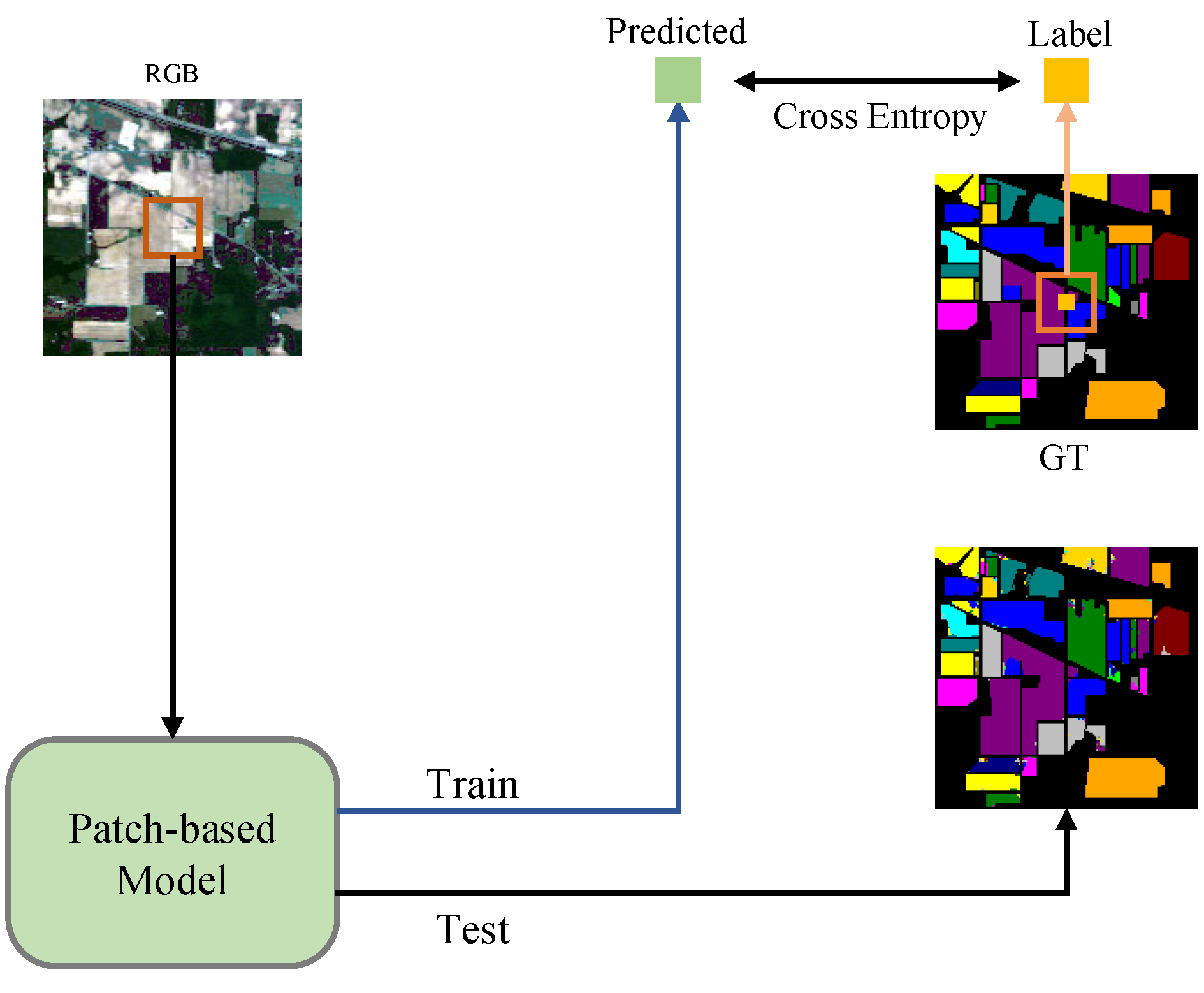
Regarding the patch-based methods, we used the principal component analysis (PCA) method to reduce the dimensionality of the dataset to a specific size. Specifically, for 1DCNN [16], we set the patch size to 1 and the number of principal components to 18. For 3DCNN [17] and Hybrid [15], we set the patch size to 15 and the number of principal components to 18. For SSFTT [12], we set the patch size to 11 and the number of principal components to 30.

3.2. Datasets

Indian Pines. The Indian Pines dataset was captured at a farm test site in northwest Indiana and collected using AVIRIS, an onboard sensor. The band range of the data set was 400–2500 nm, the spatial resolution was 20 m, and the original size of the image was 145 × 145. In this paper, the data of 200 bands were classified after water absorption and low signal-to-noise ratio bands were eliminated. During the experiment, 10% of each type of ground objects was randomly selected for training, and the remaining samples were used for testing. When the number of selected samples of each type of ground object was less than 5, we set it to 5. The specific training samples and test samples are shown in

Table 2. The number of training and testing pixels per category in the IA dataset.

No.	Class	Train	Test	Total
1	Alfalfa	5	41	46
2	Corn-notill	143	1285	1428
3	Corn-mintill	83	747	830
4	Corn	24	213	237
5	Grass-pasture	49	434	483
6	Grass-trees	73	657	730
7	Grass-pasture-mowed	5	23	28
8	Hay-windrowed	48	430	478
9	Oats	5	15	20
10	Soybean-notill	98	874	972
11	Soybean-mintill	246	2209	2455
12	Soybean-clean	60	533	593
13	Wheat	21	184	205
14	Woods	127	1138	1265
15	Buildings-Grass-Trees	39	347	386
16	Stone-Steel -Towers	10	83	93
Total		1036	9213	10,249

.

Pavia University. The dataset of Pavia University (PU) was shot in the University of Pavia, northern Italy, and was collected by airborne sensor ROSIS. The spatial resolution was 1.3 m, and the original image size was 610 × 340. In this paper, the data of 103 bands were classified by eliminating the bands affected by noise. Compared with the Indian Pines dataset, this dataset has a larger sample size and fewer categories. During the experiment, 3% of each type of ground objects were randomly selected for training, and the remaining samples were used for testing. The specific training samples and test samples are shown in

Table 3. The number of training and testing pixels per category in the PU dataset.

No.	Class	Train	Test	Total
1	Asphalt	199	6432	6631
2	Meadows	560	18,089	18,649
3	Gravel	63	2036	2099
4	Trees	92	2972	3064
5	Metal sheets	41	1304	1345
6	Bare Soil	151	4878	5029
7	Bitumen	40	1290	1330
8	Bricks	111	3671	3682
9	Shadows	29	918	947
Total		1286	41,490	42,776

.

Salinas. The Salinas (SA) dataset was taken in the Salinas Valley, California, USA, and, like the India dataset, was collected using the airborne sensor AVIRIS. However, unlike Indian Pines, it has a spatial resolution of 3.7 m. During the experiment, 1% of each type of ground objects were randomly selected for training, and the remaining samples were used for testing. The specific training samples and test samples are shown in

Table 4. The number of training and testing pixels per category in the SA dataset.

No.	Class	Train	Test	Total
1	Brocoli-green-weeds-1	21	1988	2009
2	Brocoli-green-weeds-2	38	3688	3726
3	Fallow	20	1956	1976
4	Fallow-rough-plow	14	1380	1394
5	Fallow-smooth	27	2651	2678
6	Stubble	40	3919	3959
7	Celery	36	3543	3579
8	Grapes-untrained	113	11,158	11,271
9	Soil-vinyard-develop	63	6140	6203
10	Corn-senesced-green-weeds	33	3245	3278
11	Lettuce-romaine-4wk	11	1057	1068
12	Lettuce-romaine-5wk	20	1907	1927
13	Lettuce-romaine-6wk	10	906	916
14	Lettuce-romaine-7wk	11	1059	1070
15	Vinyard-untrained	73	7195	7268
16	Vinyard-vertical-trellis	19	1788	1807
Total		549	53,580	54,129

.

3.3. Comparative Experiment

We conducted a comparative evaluation of various methods for hyperspectral image classification using a publicly available dataset. The results are presented in

Table 5. Classification accuracy (%) of the IA image with different methods.

No.	1DCNN	3DCNN	Hybird	SSFTT	Unet	FPN	Deeplabv3	Deeplabv3+	ConvNeXt	Swin	SegFormer	ResT	PVT	PoolFormer	SGHViT-S
1	41.304	89.130	100.000	97.826	50.000	93.478	95.652	82.609	89.130	89.130	89.130	84.783	97.826	89.130	97.826
2	71.218	88.305	97.269	97.829	97.899	98.459	98.109	97.129	99.510	97.129	98.810	99.020	98.739	94.048	99.370
3	57.831	91.205	97.108	97.831	95.060	96.988	96.988	96.386	93.012	96.386	97.711	96.386	96.506	94.458	96.867
4	42.616	58.650	96.625	96.203	91.561	99.156	91.983	99.578	94.937	98.312	97.468	97.890	98.734	96.624	100.000
5	86.750	96.273	98.758	99.586	95.445	98.137	98.344	99.172	97.309	92.754	98.551	97.308	99.586	98.137	99.586
6	96.986	99.041	99.315	99.452	95.890	96.849	98.767	98.767	99.863	97.945	98.767	97.808	97.534	97.123	100.000
7	75.000	75.000	100.000	100.000	57.143	100.000	100.000	100.000	100.000	100.000	100.000	100.000	100.000	100.000	100.000
8	98.745	100.000	100.000	100.000	96.653	99.372	99.791	100.000	100.000	99.582	99.582	100.000	100.000	99.582	100.000
9	30.000	65.000	90.000	100.000	70.000	100.000	100.000	100.000	100.000	100.000	100.000	100.000	100.000	100.000	100.000
10	70.576	90.021	98.868	97.634	95.062	99.177	99.691	98.457	97.531	98.045	99.794	95.267	98.765	98.971	99.691
11	80.693	96.660	99.348	98.860	98.778	98.982	98.819	99.104	98.045	97.556	99.104	98.289	96.741	98.534	99.226
12	64.250	77.403	93.592	95.784	96.796	98.314	95.110	96.965	98.651	95.616	96.627	97.639	97.470	99.831	98.145
13	96.098	83.415	100.000	100.000	91.220	100.000	99.512	98.537	100.000	97.561	100.000	100.000	100.000	100.000	100.000
14	92.648	96.364	99.763	99.842	99.763	99.526	99.605	100.000	99.447	99.684	100.000	99.605	100.000	100.000	99.921
15	50.000	91.969	94.042	97.928	88.860	99.741	100.000	100.000	99.741	99.223	100.000	99.741	99.741	99.223	100.000
16	80.645	89.247	100.000	100.000	80.645	98.925	98.925	96.774	96.774	95.699	93.548	93.548	94.624	94.624	97.849
OA	77.353	92.038	98.292	98.527	96.302	98.654	98.448	98.497	98.175	97.531	98.878	98.058	98.205	97.746	99.278
AA	70.959	86.730	97.792	98.673	87.548	98.569	98.205	97.717	97.747	97.163	98.068	97.330	98.517	97.518	99.280
K	74.100	90.897	98.053	98.321	95.780	98.465	98.232	98.287	97.921	97.187	98.721	97.787	97.955	97.431	99.177
params	−	−	−	−	33.141	26.734	40.256	27.299	29.202	14.271	14.299	14.085	14.979	22.318	2.057
flops	−	−	−	−	8.195	7.026	19.961	7.569	3.111	2.753	2.288	1.729	2.370	3.060	7.137

,

Table 6. Classification accuracy (%) of the PU image with different methods.

No.	1DCNN	3DCNN	Hybird	SSFTT	Unet	FPN	Deeplabv3	Deeplabv3+	ConvNeXt	Swin	SegFormer	ResT	PVT	PoolFormer	SGHViT-S
1	91.072	98.492	98.175	99.231	98.794	98.477	96.863	98.944	99.925	99.608	99.668	94.752	93.742	99.879	99.970
2	98.027	99.979	99.957	99.737	99.759	99.984	99.930	99.973	99.190	99.968	99.968	99.598	94.799	100.000	99.989
3	66.937	89.757	98.237	99.285	94.664	100.000	99.047	99.524	99.809	100.000	99.762	96.570	99.952	100.000	100.000
4	87.304	94.713	94.615	98.140	96.540	92.950	77.350	90.960	91.482	95.463	97.781	93.832	95.431	95.561	98.205
5	99.703	100.000	99.703	100.000	98.736	97.175	95.316	96.283	99.703	99.851	100.000	99.851	89.145	99.628	100.000
6	86.797	99.423	98.012	99.801	100.000	100.000	100.000	100.000	100.000	100.000	100.000	99.940	100.000	100.000	100.000
7	76.165	94.211	99.850	99.474	99.850	99.850	99.023	99.850	99.398	99.850	100.000	99.474	98.722	99.699	100.000
8	88.512	92.966	91.662	97.637	98.343	97.909	96.469	96.089	99.430	99.484	99.457	84.329	93.373	97.827	99.864
9	97.043	75.396	98.099	98.733	89.006	92.503	67.582	90.391	95.354	96.093	98.205	95.248	98.310	94.509	99.050
OA	91.867	97.478	98.219	99.327	98.766	98.812	96.615	98.483	98.836	99.460	99.677	96.919	95.444	99.334	99.829
AA	87.951	93.882	97.590	99.115	97.299	97.650	92.398	96.890	98.255	98.924	99.427	95.955	95.942	98.567	99.675
K	89.149	96.648	97.635	99.108	98.367	98.426	95.507	97.988	98.457	99.284	99.572	95.919	94.035	99.116	99.774
params	−	−	−	−	32.836	26.429	39.950	26.993	29.052	14.121	13.993	14.056	14.675	22.014	1.939
flops	−	−	−	−	54.759	44.668	158.734	49.431	25.253	21.427	15.825	13.661	16.550	22.623	36.180

and

Table 7. Classification accuracy (%) of the SA image with different methods.

No.	1DCNN	3DCNN	Hybird	SSFTT	Unet	FPN	Deeplabv3	Deeplabv3+	ConvNeXt	Swin	SegFormer	ResT	PVT	PoolFormer	SGHViT-S
1	98.805	99.204	100.000	99.552	95.669	99.851	98.855	100.000	99.004	99.801	100.000	99.104	100.000	99.452	100.000
2	99.597	99.973	100.000	100.000	100.000	99.249	99.919	100.000	99.678	99.758	100.000	99.919	99.678	99.463	100.000
3	98.785	99.038	99.949	100.000	92.864	100.000	100.000	100.000	99.494	100.000	100.000	99.899	99.494	100.000	100.000
4	98.852	95.768	98.924	99.785	90.961	92.611	96.270	100.000	98.780	100.000	100.000	100.000	98.780	99.641	99.857
5	95.930	95.519	98.432	99.813	90.403	99.664	96.079	99.776	98.021	96.565	99.813	98.954	99.178	98.170	99.515
6	99.773	99.899	98.687	100.000	99.747	99.874	97.247	99.798	99.949	99.874	100.000	99.646	100.000	99.545	100.000
7	99.329	99.497	100.000	99.888	96.899	99.665	98.128	99.916	99.637	99.329	100.000	99.888	99.441	99.832	100.000
8	82.113	96.469	98.341	98.199	99.379	99.965	99.574	99.752	99.991	99.565	99.947	99.973	99.973	99.911	99.840
9	99.936	99.936	100.000	100.000	99.613	100.000	100.000	100.000	100.000	100.000	100.000	100.000	100.000	100.000	100.000
10	91.245	97.224	98.780	99.664	96.888	97.010	99.634	97.590	100.000	100.000	98.841	99.786	99.939	99.512	99.847
11	86.704	92.603	98.596	99.157	91.760	100.000	98.689	100.000	100.000	100.000	100.000	100.000	100.000	100.000	100.000
12	99.844	99.948	99.222	99.844	91.801	96.990	94.136	96.419	94.551	96.938	99.273	97.094	97.613	97.353	99.948
13	83.297	95.961	99.891	98.144	57.860	95.742	75.873	90.066	99.782	99.782	100.000	100.000	100.000	99.127	100.000
14	93.551	98.318	97.477	99.346	92.523	91.215	96.355	99.720	98.785	97.196	100.000	91.776	94.953	96.636	99.720
15	69.056	91.194	96.395	94.950	99.532	99.917	97.936	98.101	97.826	98.170	99.367	95.638	99.408	99.051	99.972
16	95.517	89.983	99.281	97.178	81.350	99.889	100.000	99.945	100.000	100.000	100.000	100.000	100.000	100.000	99.668
OA	90.347	96.885	98.762	98.727	96.285	99.148	98.234	99.213	99.250	99.248	99.799	99.002	99.577	99.448	99.908
AA	93.271	96.908	98.998	99.095	92.328	98.228	96.793	98.818	99.094	99.186	99.828	98.855	99.279	99.231	99.898
K	89.247	96.529	98.622	98.582	95.856	99.052	98.033	99.124	99.165	99.163	99.776	98.889	99.529	99.385	99.897
params	−	−	−	−	18.372	11.420	40.268	27.312	29.195	28.869	14.298	14.069	14.977	22.331	2.059
flops	−	−	−	−	38.893	34.624	89.783	34.205	13.959	14.097	10.323	7.757	10.692	13.816	32.541

. Our analysis showed that the patch-based approach is not very effective for hyperspectral image classification. Ordinary 1DCNN and 3DCNN models have difficulties classifying ground objects with similar spectral characteristics. However, Hybrid, which combines 2DCNN and 3DCNN, can mitigate this limitation to some extent.

We also evaluated SSFTT, which uses a combination of Transformer and CNN to fully extract spatial and spectral features. However, this method is limited by patch-based data-processing methods, which restrict its ability to model the global scene effectively. In contrast, semantic segmentation-based methods can make good use of spatial features for global scene modeling. Nevertheless, most of these methods were designed for three-channel images and did not fully consider the spectral dimension. Additionally, traditional semantic segmentation methods tended to focus on regional features, which could make it challenging to extract deep semantic features. Although models like Unet, FPN, and Deeplabv3 were widely used for various computer vision tasks, they did not perform optimally for hyperspectral semantic segmentation. Moreover, these models tend to have a large number of parameters, which can lead to higher computational costs and memory requirements. In contrast, SGHViT had promising results on hyperspectral semantic segmentation tasks while utilizing significantly fewer parameters and moderate floating-point operations per second (FLOPS). Thus, SGHViT was a more effective choice for hyperspectral semantic segmentation tasks.

Transformer-based models showed promising results for hyperspectral semantic segmentation tasks. This is attributed to Transformer’s ability to extract features effectively and model spectral dimension information accurately. Swin, SegFormer, ResT, and other Transformer-based models demonstrated impressive potential in hyperspectral semantic segmentation tasks. In particular, SegFormer achieved comparable results to our proposed model on the three datasets, indicating that a simple decoder could often achieve a better performance for hyperspectral semantic segmentation tasks.

To further improve the performance of our proposed model, we designed a novel decoder architecture that efficiently the transmitted texture information extracted by the upper layers of the model to the decoder. This reduced the misclassification of the model and enhanced its segmentation accuracy. In the ablation experiment section, we compared our decoder architecture with UperNet, and the results demonstrated the effectiveness of our proposed approach.

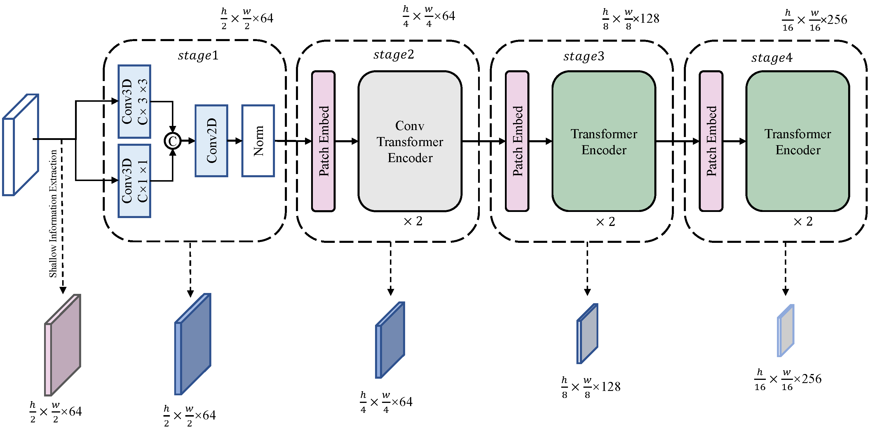
It is worth noting that PoolFormer is a hierarchical model that uses simple pooling modules. It achieved good results on the three datasets, which further confirms the importance of the hierarchical structure in hyperspectral image classification. In our study, we also adopted the traditional hierarchical structure and used stages 1–4 to represent the model structure.

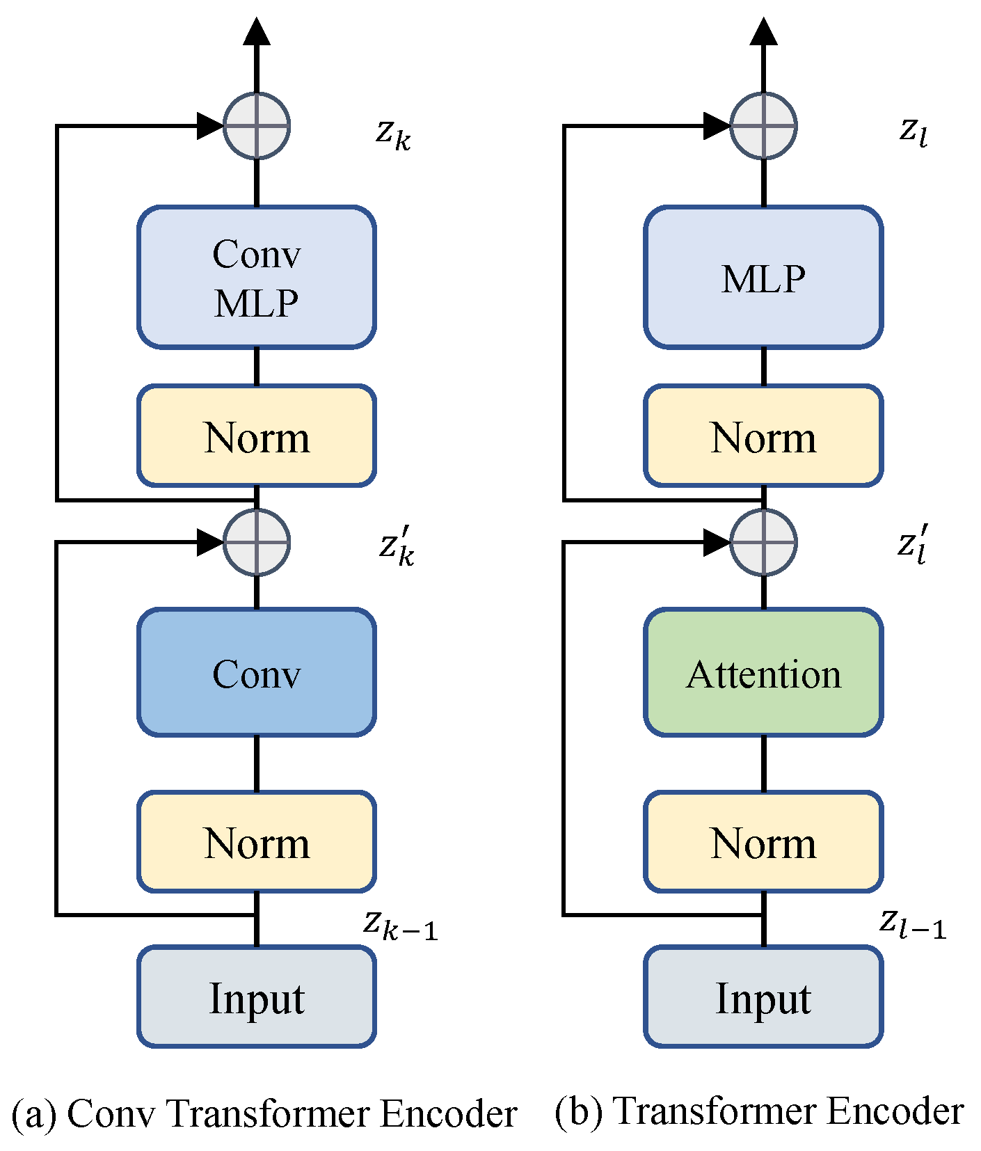
The ConvNeXt experiment provided additional evidence supporting the importance of the hierarchical structure for hyperspectral semantic segmentation tasks. We found that pure convolution-based Transformer-like models cannot fully extract deep semantic information, and therefore cannot achieve a good segmentation performance. To address this limitation, our model combines CNN and Transformer layers to extract shallow and deep information, respectively. Specifically, we used CNN to extract shallow information in the early layers of the model, and Transformer to extract deep information in the later layers.

Our analysis of the AA showed that our proposed method could effectively leverage the shallow spatial detail information of hyperspectral images. Specifically, the shallow layer information extraction module significantly enhanced the model’s ability to extract texture information. At the same time, the segmentation accuracy of the model was also enhanced, and the location of the ground objects generated by the model was limited to the effective area. The incorporation of the Decoder part, which operated on the output of the Transformer layer, further improved the segmentation accuracy of our model. The Decoder part effectively refined the output of the model and ensured that the predicted ground objects were within the valid area of the image. As a result, the AA of our model was significantly higher than other, similar models.

Based on the results presented in Table 5 and Figure 6, SGHViT achieved the highest classification accuracy for most ground objects in the IA dataset, with some objects reaching 100%. However, for certain objects, such as alfalfa, corn-notill, corn-mintill, soybean-clean, and stone-Steel-Towers, SGHViT did not achieve optimal results, with a gap of approximately ∼2% compared to the best-performing model. This is because SGHViT needs to fully consider the distribution of various ground objects for classification. The location of these features is concentrated and often difficult to distinguish at the edge. Figure 6 indicates that 1DCNN and Unet had a high number of misclassifications, while 3DCNN exhibited many misclassifications in certain areas. Hybrid models improved a substantial number of misclassifications, and SSFTT only had misclassifications in the edge areas of ground objects. Models such as FPN, Deeplabv3, and Swin only showed misclassifications for some challenging features. Although SGHViT also exhibits misclassifications for some difficult-to-classify objects, it outperforms the semantic segmentation-based methods, improving classification accuracy for most areas.

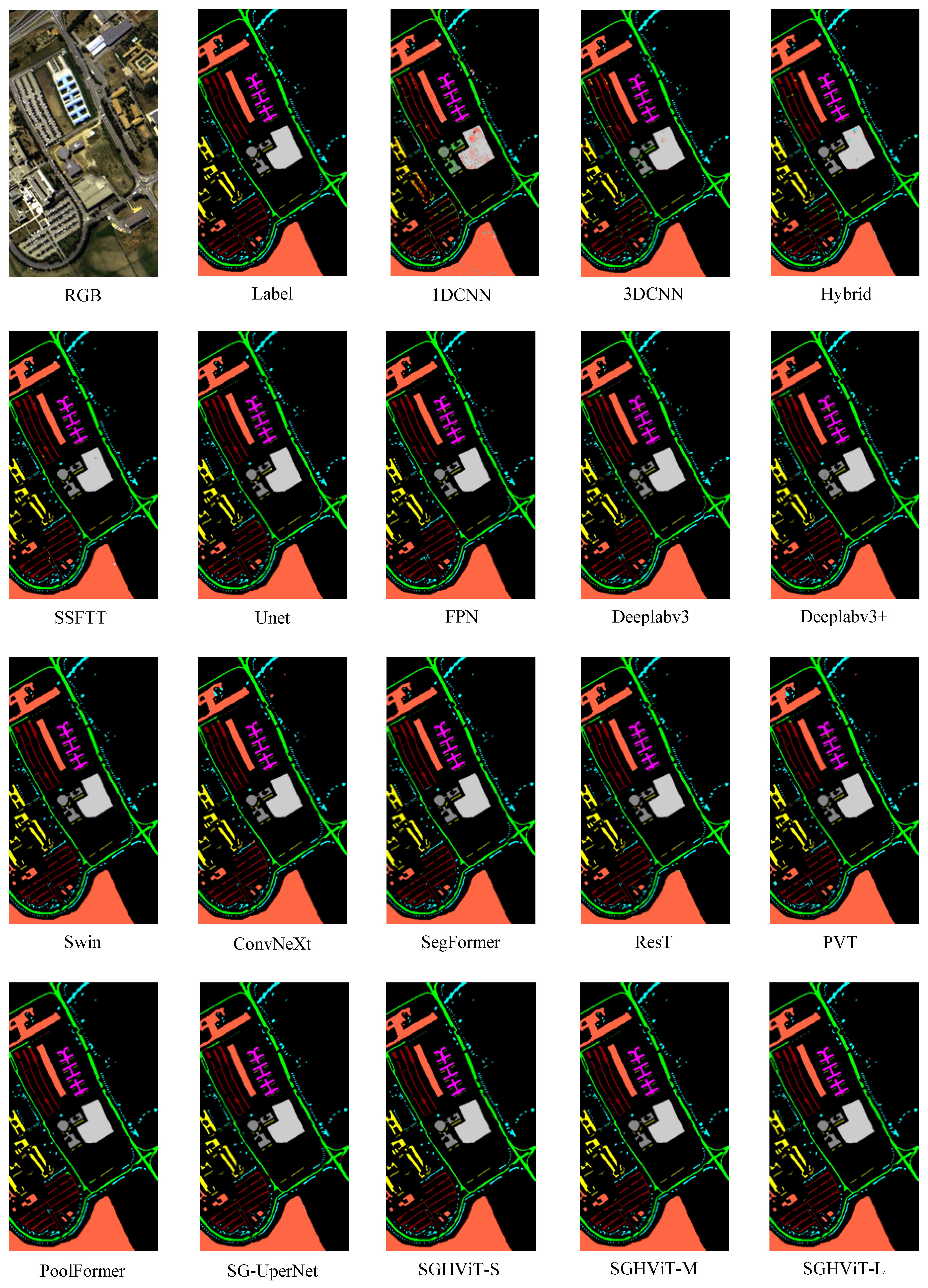
According to the results presented in Table 6 and Figure 7, SGHViT achieved the best classification accuracy for almost all ground objects in the PU dataset. Specifically, SGHViT achieved 100% accuracy for Gravel, Metal sheets, Bare Soil, and Bitumen, and was only slightly worse than the best-performing model for Meadows, by approximately ∼0.1%. Figure 7 indicates that patch-based methods did not perform well on the challenging PU dataset, with all methods exhibiting misclassifications in the central area of ground objects. However, semantic segmentation-based methods had no misclassifications in the central region of Bare Soil and other objects. Unet, Deeplabv3, and SegFormer exhibit numerous misclassifications for Asphalt, Shadows, and Trees, whereas SGHViT significantly improves the misclassification of these features, especially Trees and Shadows. Overall, SGHViT demonstrates reasonable classification accuracy for different ground objects and outperforms other methods in terms of comprehensive indicators such as OA, AA, and K.

Evidenced by the results presented in Table 7 and Figure 8, SGHViT achieves the best classification accuracy for most ground objects in the SA dataset, with the exception of fallow-rough-plow, grapes-untrained, corn-senesced-green-weeds, lettuce-romaine-7wk, and vinyard-vertical-trellis.SGHViT achieves 100% accuracy for multiple ground objects. Figure 8 clearly shows a significant number of misclassifications in the patch-based and Unet methods. However, other models based on semantic segmentation exhibit partial misclassifications for Vinyard_u, Grapes, Lettuce_4wk, Lettuce_5wk, Lettuce_6wk, Lettuce_7wk, and Corn, which are particularly noticeable at the edge between Vinyard_u and Grapes. SGHViT effectively overcomes the aforementioned misclassification issues, exhibiting very few misclassifications for difficult-to-classify objects such as Vinyard_u and Grapes.

3.4. Ablation Experiment

We present the results of the ablation experiments in

Table 8. Backbone experiments on different Decoders and different numbers of Transformer blocks.

No.	IA				PU				SA
	SG-UperNet	SGHViT-S	SGHViT-M	SGHViT-L	SG-UperNet	SGHViT-S	SGHViT-M	SGHViT-L	SG-UperNet	SGHViT-S	SGHViT-M	SGHViT-L
1	91.304	97.826	97.826	97.826	98.492	99.970	100.000	100.000	100.000	100.000	100.000	100.000
2	99.510	99.370	99.090	99.020	100.000	99.989	99.984	100.000	100.000	100.000	100.000	100.000
3	97.470	96.867	97.711	98.072	100.000	100.000	99.714	100.000	100.000	100.000	100.000	100.000
4	100.000	100.000	100.000	100.000	98.042	98.205	98.401	98.597	99.857	99.857	100.000	99.713
5	98.344	99.586	99.586	99.586	100.000	100.000	100.000	100.000	98.954	99.515	99.963	100.000
6	98.219	100.000	99.863	99.863	100.000	100.000	100.000	100.000	100.000	100.000	100.000	100.000
7	100.000	100.000	100.000	100.000	100.000	100.000	100.000	100.000	100.000	100.000	99.972	99.972
8	100.000	100.000	100.000	100.000	99.946	99.864	99.946	100.000	99.796	99.840	99.920	99.973
9	100.000	100.000	100.000	100.000	100.000	99.050	99.578	99.894	100.000	100.000	100.000	100.000
10	99.588	99.691	99.794	99.588	−	−	−	−	100.000	99.847	99.908	99.908
11	98.819	99.226	99.226	99.470	−	−	−	−	100.000	100.000	99.906	100.000
12	96.965	98.145	98.145	98.820	−	−	−	−	99.948	99.948	100.000	99.741
13	100.000	100.000	100.000	100.000	−	−	−	−	100.000	100.000	100.000	100.000
14	99.921	99.921	99.921	100.000	−	−	−	−	95.234	99.720	98.879	99.813
15	100.000	100.000	100.000	100.000	−	−	−	−	99.959	99.972	99.862	99.904
16	97.849	97.849	97.849	97.849	−	−	−	−	100.000	99.668	99.723	100.000
OA	98.956	99.278	99.307	99.415	99.621	99.829	99.850	99.897	99.800	99.908	99.922	99.954
AA	98.624	99.280	99.313	99.381	99.609	99.675	99.736	99.832	99.609	99.898	99.883	99.939
K	98.810	99.177	99.210	99.333	99.498	99.774	99.802	99.864	99.778	99.897	99.914	99.949
params	2.176	2.057	3.093	3.891	2.057	1.939	2.974	3.773	2.278	2.059	3.093	3.889
flops	8.340	7.137	7.365	7.683	46.766	36.180	38.190	40.989	37.916	32.541	33.564	34.983

and

Table 9. Ablation experiments on three datasets.

Module			IA					PU					SA
Shallow	Pos	Fusion	Params	Flops	OA	AA	K	Params	Flops	OA	AA	K	Params	Flops	OA	AA	K
✗	✔	✔	1.942	4.187	98.927	98.758	98.776	1.879	22.815	99.696	99.420	99.597	1.944	19.050	99.832	99.838	99.812
✔	✗	✔	2.049	7.138	99.199	99.087	99.087	1.931	36.191	99.764	99.567	99.686	2.054	32.532	99.847	99.867	99.829
✔	✔	✗	1.942	7.118	99.171	99.087	99.054	1.824	36.020	99.752	99.625	99.671	1.947	32.445	99.828	99.756	99.808
✗	✗	✔	1.937	4.186	98.868	98.711	98.710	1.875	22.801	99.633	99.206	99.513	1.940	19.043	99.826	99.699	99.806
✗	✔	✗	1.827	4.168	98.810	99.036	98.643	1.765	22.655	99.460	99.273	99.284	1.830	18.968	99.754	99.852	99.726
✔	✗	✗	1.938	7.116	99.258	98.965	99.154	1.820	36.006	99.733	99.688	99.646	1.943	32.438	99.762	99.830	99.734
✗	✗	✗	1.823	4.167	98.849	98.715	98.687	1.760	22.641	99.425	99.008	99.238	1.825	18.961	99.728	99.804	99.697

, where we comprehensively evaluated the impact of different modules on the performance of the model. Specifically, we investigated the effect of stacking Transformer blocks on the model’s performance, as well as the performance impact of our designed Decoder compared to the widely used UperNet [13,49].

(1)

The impact of using different Decoders on the SGHViT backbone.

We evaluated the use of UperNet as the Decoder of our model, and present the results in Table 8. Specifically, we designed an SG-UperNet model that used SGHViT-S as the backbone and UperNet as the Decoder. Our results showed that using SGHViT-S as the backbone, combined with UperNet, could achieve good results for hyperspectral semantic segmentation tasks. This reflected the ability of SGHViT-S to effectively extract both shallow and deep semantic information from hyperspectral images and model both local and global context.

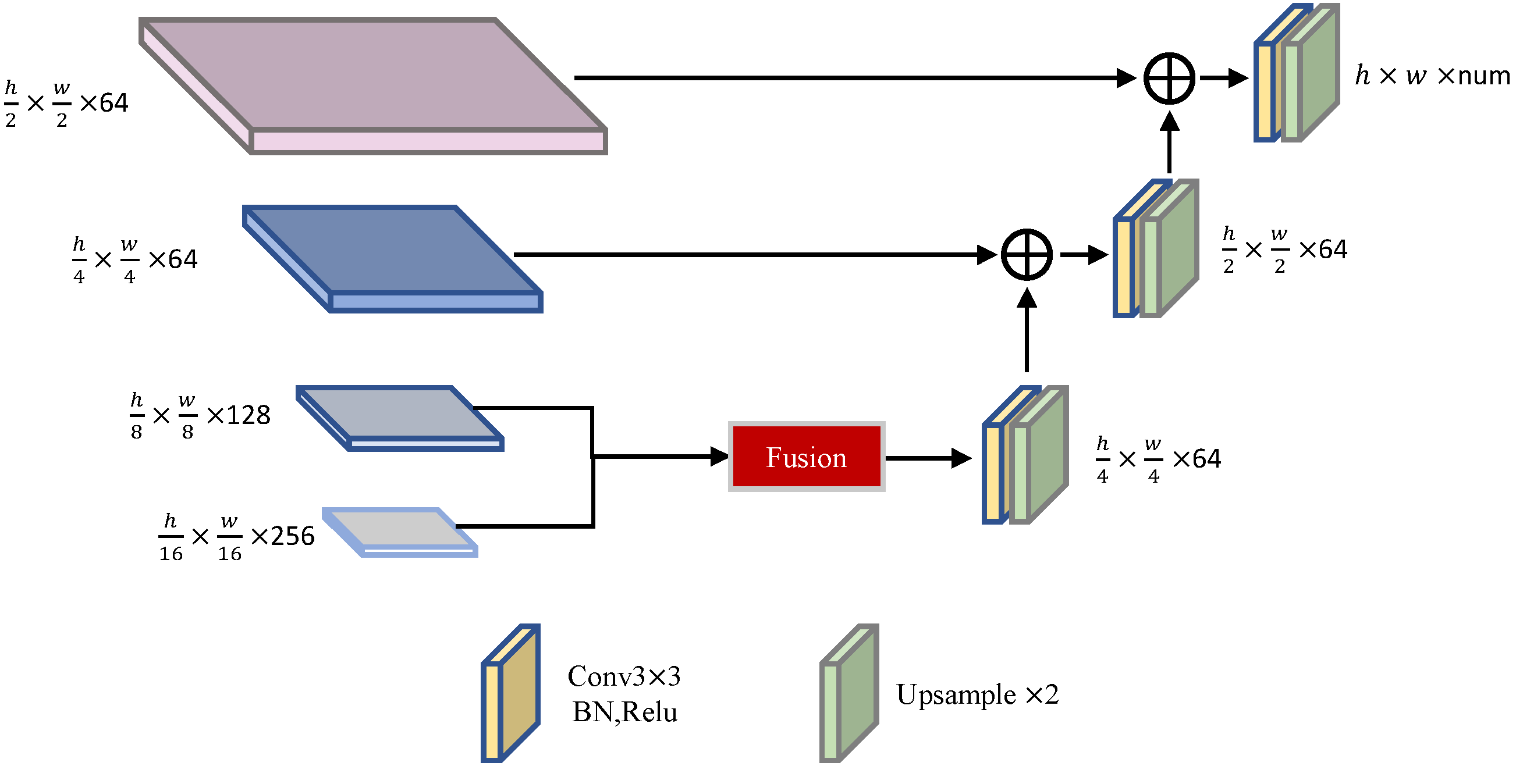
However, using UperNet as the Decoder could result in a high parameter quantity and computational complexity. To address this, we proposed a simplified LinkNet-like Decoder that could achieve comparable results with a lower computational cost. Our proposed method used the feature maps of stage3 and stage4 from the Transformer module for feature aggregation, and then applied our simplified Decoder to generate the final segmentation map.

(2)

The effect of using different numbers of Transformer blocks on the SGHViT backbone.

We evaluated the effect of stacking Transformer blocks on the performance of our model, and the specific results are presented in Table 8. Specifically, we investigated the impact of varying the number of components of SGHViT-S, SGHViT-M, and SGHViT-L, with the number of components set to [1, 1, 1], [2, 2, 2], and [2, 6, 2], respectively.

Our experimental results showed that, as the number of stacked Transformer blocks increased, the performance of our model improved on all three datasets. This demonstrated the effectiveness of our method in leveraging the multi-scale context information of hyperspectral images.

(3)

The effect of different components.

We conducted ablation experiments to evaluate the impact of different modules on the performance of our model for hyperspectral semantic segmentation tasks. Specifically, we evaluated the relative position encoding module (Pos), shallow feature extraction module (Shallow), and feature aggregation module (Fusion).

Our results showed that the relative position encoding module improved the performance of the model in the classification of lower hyperspectral ground objects and had a positive impact on all three datasets. The shallow feature extraction module also had a crucial impact on the correct classification of ground objects, particularly for dense prediction tasks. The OA, AA, and K indicators of the model without the shallow feature extraction module showed a significant decline, especially on the AA indicator. This highlighted the importance of incorporating shallow spatial detail features in the model to reduce misclassifications.

We also found that the feature aggregation module had a significant impact on hyperspectral images with high spatial resolution. For lower-resolution images, the effect of the module was not as significant. However, the module significantly improved various performance indicators for high-resolution images, which was consistent with the module’s design goal. This demonstrated the necessity of feature aggregation processing on the feature maps extracted by Transformer, as discussed in the previous literature [38].

3.5. Comparative Experiments on Other Datasets

To further evaluate the effectiveness of our method, we compared it with several representative models on two challenging datasets, namely the Pavia Center and Botswana datasets. The experimental results of these comparisons were presented in

Table 10. Comparative experiments on other datasets.

Method	Pavia Center			Botswana
	OA	AA	K	OA	AA	K
Hybrid	97.722	92.875	96.769	91.478	91.062	90.770
SSFTT	98.550	95.012	97.946	96.468	95.655	96.172
FPN	94.390	81.345	97.723	99.261	99.288	99.200
Swin	95.855	86.713	94.120	99.569	99.602	99.533
SegFormer	96.670	89.335	95.278	99.938	99.943	99.933
SG-UperNet	98.116	94.763	97.334	99.969	99.977	99.967
SGHViT-S	98.812	96.345	98.317	100.000	100.000	100.000

. For the Pavia Center dataset, we used 0.2% of the total samples for training and the remaining 99.8% for testing. Similarly, for the Botswana dataset, we randomly selected 5% of the data for training and the remaining 95% for testing. To ensure the effective execution of our method on the device, we replaced the multi-head self-attention in the Transformer Encoder at Stages 3 and 4 with window-based self-attention. Window-based self-attention restricted the attention mechanism to a fixed-size window around each token, reducing the computational complexity of the self-attention operation and improving the efficiency of the model. However, this also limited the ability of tokens to attend to distant information in the sequence. Despite this limitation, our method demonstrated a superior performance on these challenging datasets, which demonstrated the reliability and superiority of the SGHViT architecture, especially in scenarios with limited training data.

3.6. Robustness Evaluation

We evaluated the robustness of SGHViT by conducting experiments on our proposed model and several representative models under different numbers of training samples. Figure 9 showed the experimental results on the three datasets. We varied the number of training samples by selecting 2%, 4%, 6%, 8% and 10% of the samples for the IA dataset, 0.5%, 1%, 1.5%, 2% and 3% of the samples for the PU dataset, and 0.2%, 0.4%, 0.6%, 0.8% and 1% of the samples for the SA dataset.

Our results showed that SGHViT outperformed other models in all cases. As the number of training samples decreased, SGHViT achieved higher accuracy compared to other models. This reflected the robustness of SGHViT in small-sample scenarios, where it could achieve a superior performance, even with extremely limited training data.

4. Conclusions

In this paper, we explore the possibility of using hierarchical Transformers in hyperspectral semantic segmentation tasks. We designed a backbone for the hyperspectral semantic segmentation task. The hyperspectral space and spectral features are fully extracted through the shallow-information feature-extraction module and the spectral feature-extraction module. The conv Transformer Encoder and Transformer Encoder were used in appropriate locations to effectively combine CNN and Transformer. At the same time, we designed a simple Decoder, which allows the model to achieve remarkable results in the hyperspectral semantic segmentation task. We conducted detailed comparison experiments with mainstream hierarchical Transformer models, traditional semantic segmentation models, and Patch-based methods. The experimental results show that the hierarchical Transformer has great potential in the field of hyperspectral remote sensing due to its advantages of high precision and low computational cost.

Although the SGHViT model presented in this paper demonstrates excellent hyperspectral object classification performance, the introduction of Transformers for feature extraction enhances the model’s capacity to model long-range dependencies and capture global context information, thus improving segmentation performance. However, this improvement comes at the cost of an increase in the number of model parameters and computational complexity. Therefore, future research efforts will focus on designing lightweight models that balance performance and efficiency.

In addition, we did not consider introducing Transformers into the Decoder component of the model. Future research will continue to explore the application of lightweight models in hyperspectral object classification tasks and investigated how to effectively integrate Transformers into the Decoder to improve the model’s ability to capture spatial information. Specifically, we will investigate techniques for reducing the computational cost of incorporating Transformers into the Decoder, such as knowledge distillation and model compression.

Overall, the successful application of Transformers in hyperspectral object classification tasks highlights their potential for improving the performance of deep learning models in the hyperspectral domain. However, the increased computational cost of using Transformers underscores the need for more efficient model designs. Future research efforts will focus on developing lightweight models that balance performance and efficiency while exploring the potential benefits of integrating Transformers into the Decoder component of the model.

References

1. Cai, Y.; Lin, J.; Hu, X.; Wang, H.; Yuan, X.; Zhang, Y.; Timofte, R.; Van Gool, L. Mask-guided spectral-wise transformer for efficient hyperspectral image reconstruction. In Proceedings of the IEEE/CVF Conference on Computer Vision and Pattern Recognition, New Orleans, LA, USA, 18–24 June 2022; pp. 17502–17511. [Google Scholar]
2. Hu, M.; Wu, C.; Zhang, L. HyperNet: Self-supervised hyperspectral spatial–spectral feature understanding network for hyperspectral change detection. IEEE Trans. Geosci. Remote Sens. 2022, 60, 5543017. [Google Scholar] [CrossRef]
3. Tian, S.; Lu, Q.; Wei, L. Multiscale Superpixel-Based Fine Classification of Crops in the UAV-Based Hyperspectral Imagery. Remote Sens. 2022, 14, 3292. [Google Scholar] [CrossRef]
4. Zhou, L.; Zhang, C.; Wu, M. D-LinkNet: LinkNet with pretrained encoder and dilated convolution for high resolution satellite imagery road extraction. In Proceedings of the IEEE Conference on Computer Vision and Pattern Recognition Workshops, Salt Lake City, UT, USA, 18–22 June 2018; pp. 182–186. [Google Scholar]
5. Li, R.; Zheng, S.; Zhang, C.; Duan, C.; Wang, L.; Atkinson, P.M. ABCNet: Attentive bilateral contextual network for efficient semantic segmentation of Fine-Resolution remotely sensed imagery. ISPRS J. Photogramm. Remote Sens. 2021, 181, 84–98. [Google Scholar] [CrossRef]
6. Ding, X.; Zhang, X.; Han, J.; Ding, G. Scaling up your kernels to 31 × 31: Revisiting large kernel design in cnns. In Proceedings of the IEEE/CVF Conference on Computer Vision and Pattern Recognition, New Orleans, LA, USA, 18–24 June 2022; pp. 11963–11975. [Google Scholar]
7. Chen, Y.; Wang, B.; Yan, Q. Hyperspectral Remote-Sensing Classification Combining Transformer and Multiscale Residual Mechanisms. Laser Optoelectron. Prog. 2023, 60, 1228002. [Google Scholar]
8. Dosovitskiy, A.; Beyer, L.; Kolesnikov, A.; Weissenborn, D.; Zhai, X.; Unterthiner, T.; Dehghani, M.; Minderer, M.; Heigold, G.; Gelly, S.; et al. An image is worth 16 × 16 words: Transformers for image recognition at scale. arXiv 2020, arXiv:2010.11929. [Google Scholar]
9. Zhong, Z.; Li, Y.; Ma, L.; Li, J.; Zheng, W.S. Spectral–spatial transformer network for hyperspectral image classification: A factorized architecture search framework. IEEE Trans. Geosci. Remote Sens. 2021, 60, 5514715. [Google Scholar] [CrossRef]
10. Hong, D.; Han, Z.; Yao, J.; Gao, L.; Zhang, B.; Plaza, A.; Chanussot, J. SpectralFormer: Rethinking hyperspectral image classification with transformers. IEEE Trans. Geosci. Remote Sens. 2021, 60, 5518615. [Google Scholar] [CrossRef]
11. Yu, H.; Xu, Z.; Zheng, K.; Hong, D.; Yang, H.; Song, M. MSTNet: A Multilevel Spectral–Spatial Transformer Network for Hyperspectral Image Classification. IEEE Trans. Geosci. Remote Sens. 2022, 60, 5532513. [Google Scholar] [CrossRef]
12. Sun, L.; Zhao, G.; Zheng, Y.; Wu, Z. Spectral–spatial feature tokenization transformer for hyperspectral image classification. IEEE Trans. Geosci. Remote Sens. 2022, 60, 5522214. [Google Scholar] [CrossRef]
13. Liu, Z.; Lin, Y.; Cao, Y.; Hu, H.; Wei, Y.; Zhang, Z.; Lin, S.; Guo, B. Swin transformer: Hierarchical vision transformer using shifted windows. In Proceedings of the IEEE/CVF International Conference on Computer Vision, Montreal, BC, Canada, 11–17 October 2021; pp. 10012–10022. [Google Scholar]
14. Peng, Y.; Ren, J.; Wang, J.; Shi, M. Spectral-Swin Transformer with Spatial Feature Extraction Enhancement for Hyperspectral Image Classification. Remote Sens. 2023, 15, 2696. [Google Scholar] [CrossRef]
15. Ghaderizadeh, S.; Abbasi-Moghadam, D.; Sharifi, A.; Zhao, N.; Tariq, A. Hyperspectral image classification using a hybrid 3D-2D convolutional neural networks. IEEE J. Sel. Top. Appl. Earth Obs. Remote Sens. 2021, 14, 7570–7588. [Google Scholar] [CrossRef]
16. Hu, W.; Huang, Y.; Wei, L.; Zhang, F.; Li, H. Deep convolutional neural networks for hyperspectral image classification. J. Sensors 2015, 2015, 258619. [Google Scholar] [CrossRef] [Green Version]
17. Hamida, A.B.; Benoit, A.; Lambert, P.; Amar, C.B. 3-D deep learning approach for remote sensing image classification. IEEE Trans. Geosci. Remote Sens. 2018, 56, 4420–4434. [Google Scholar] [CrossRef] [Green Version]
18. Gong, H.; Li, Q.; Li, C.; Dai, H.; He, Z.; Wang, W.; Li, H.; Han, F.; Tuniyazi, A.; Mu, T. Multiscale information fusion for hyperspectral image classification based on hybrid 2D-3D CNN. Remote Sens. 2021, 13, 2268. [Google Scholar] [CrossRef]
19. García, J.L.; Paoletti, M.E.; Jiménez, L.I.; Haut, J.M.; Plaza, A. Efficient Semantic Segmentation of Hyperspectral Images Using Adaptable Rectangular Convolution. IEEE Geosci. Remote Sens. Lett. 2022, 19, 6005905. [Google Scholar] [CrossRef]
20. Pan, B.; Xu, X.; Shi, Z.; Zhang, N.; Luo, H.; Lan, X. DSSNet: A Simple Dilated Semantic Segmentation Network for Hyperspectral Imagery Classification. IEEE Geosci. Remote Sens. Lett. 2020, 17, 1968–1972. [Google Scholar] [CrossRef]
21. Zhu, Q.; Deng, W.; Zheng, Z.; Zhong, Y.; Guan, Q.; Lin, W.; Zhang, L.; Li, D. A spectral-spatial-dependent global learning framework for insufficient and imbalanced hyperspectral image classification. IEEE Trans. Cybern. 2021, 52, 11709–11723. [Google Scholar] [CrossRef] [PubMed]
22. Meng, X.; Yang, Y.; Wang, L.; Wang, T.; Li, R.; Zhang, C. Class-Guided Swin Transformer for Semantic Segmentation of Remote Sensing Imagery. IEEE Geosci. Remote Sens. Lett. 2022, 19, 6517505. [Google Scholar] [CrossRef]
23. Zhu, Q.; Zhang, Y.; Wang, L.; Zhong, Y.; Guan, Q.; Lu, X.; Zhang, L.; Li, D. A global context-aware and batch-independent network for road extraction from VHR satellite imagery. ISPRS J. Photogramm. Remote Sens. 2021, 175, 353–365. [Google Scholar] [CrossRef]
24. Wang, W.; Xie, E.; Li, X.; Fan, D.P.; Song, K.; Liang, D.; Lu, T.; Luo, P.; Shao, L. Pvt v2: Improved baselines with pyramid vision transformer. Comput. Vis. Media 2022, 8, 415–424. [Google Scholar] [CrossRef]
25. Yu, W.; Luo, M.; Zhou, P.; Si, C.; Zhou, Y.; Wang, X.; Feng, J.; Yan, S. Metaformer is actually what you need for vision. In Proceedings of the IEEE/CVF Conference on Computer Vision and Pattern Recognition, New Orleans, LA, USA, 18–24 June 2022; pp. 10819–10829. [Google Scholar]
26. Liu, Z.; Mao, H.; Wu, C.Y.; Feichtenhofer, C.; Darrell, T.; Xie, S. A convnet for the 2020s. In Proceedings of the IEEE/CVF Conference on Computer Vision and Pattern Recognition, New Orleans, LA, USA, 18–24 June 2022; pp. 11976–11986. [Google Scholar]
27. Chang, S.; Wang, P.; Lin, M.; Wang, F.; Zhang, D.J.; Jin, R.; Shou, M.Z. Making Vision Transformers Efficient from a Token Sparsification View. In Proceedings of the IEEE/CVF Conference on Computer Vision and Pattern Recognition, Vancouver, BC, Canada, 18–22 June 2023; pp. 6195–6205. [Google Scholar]
28. Ding, M.; Xiao, B.; Codella, N.; Luo, P.; Wang, J.; Yuan, L. Davit: Dual attention vision transformers. In Proceedings of the Computer Vision–ECCV 2022: 17th European Conference, Tel Aviv, Israel, 23–27 October 2022; Proceedings, Part XXIV. Springer: Berlin, Germany, 2022; pp. 74–92. [Google Scholar]
29. Pan, X.; Ge, C.; Lu, R.; Song, S.; Chen, G.; Huang, Z.; Huang, G. On the integration of self-attention and convolution. In Proceedings of the IEEE/CVF Conference on Computer Vision and Pattern Recognition, New Orleans, LA, USA, 18–24 June 2022; pp. 815–825. [Google Scholar]
30. Xu, J.; Sun, X.; Zhang, Z.; Zhao, G.; Lin, J. Understanding and improving layer normalization. In Advances in Neural Information Processing Systems; MIT Press: Cambridge, MA, USA, 2019; Volume 32. [Google Scholar]
31. Sun, J.; Shen, Z.; Wang, Y.; Bao, H.; Zhou, X. LoFTR: Detector-free local feature matching with transformers. In Proceedings of the IEEE/CVF Conference on Computer Vision and Pattern Recognition, Nashville, TN, USA, 20–25 June 2021; pp. 8922–8931. [Google Scholar]
32. d’Ascoli, S.; Touvron, H.; Leavitt, M.L.; Morcos, A.S.; Biroli, G.; Sagun, L. Convit: Improving vision transformers with soft convolutional inductive biases. In Proceedings of the International Conference on Machine Learning (PMLR), Virtual, 18–24 June 2021; pp. 2286–2296. [Google Scholar]
33. Pan, Z.; Cai, J.; Zhuang, B. Fast vision transformers with hilo attention. arXiv 2022, arXiv:2205.13213. [Google Scholar]
34. Devlin, J.; Chang, M.W.; Lee, K.; Toutanova, K. Bert: Pre-training of deep bidirectional transformers for language understanding. arXiv 2018, arXiv:1810.04805. [Google Scholar]
35. Vaswani, A.; Shazeer, N.; Parmar, N.; Uszkoreit, J.; Jones, L.; Gomez, A.N.; Kaiser, Ł.; Polosukhin, I. Attention is all you need. In Advances in Neural Information Processing Systems; MIT Press: Cambridge, MA, USA, 2017; Volume 30. [Google Scholar]
36. He, X.; Chen, Y.; Lin, Z. Spatial-spectral transformer for hyperspectral image classification. Remote Sens. 2021, 13, 498. [Google Scholar] [CrossRef]
37. Strudel, R.; Garcia, R.; Laptev, I.; Schmid, C. Segmenter: Transformer for semantic segmentation. In Proceedings of the IEEE/CVF International Conference on Computer Vision, Montreal, BC, Canada, 11–17 October 2021; pp. 7262–7272. [Google Scholar]
38. Xie, E.; Wang, W.; Yu, Z.; Anandkumar, A.; Alvarez, J.M.; Luo, P. SegFormer: Simple and efficient design for semantic segmentation with transformers. In Advances in Neural Information Processing Systems; MIT Press: Cambridge, MA, USA, 2021; Volume 34, pp. 12077–12090. [Google Scholar]
39. Hendrycks, D.; Gimpel, K. Gaussian error linear units (gelus). arXiv 2016, arXiv:1606.08415. [Google Scholar]
40. Xiao, T.; Liu, Y.; Zhou, B.; Jiang, Y.; Sun, J. Unified perceptual parsing for scene understanding. In Proceedings of the European Conference on Computer Vision (ECCV), Munich, Germany, 8–14 September 2018; pp. 418–434. [Google Scholar]
41. Chaurasia, A.; Culurciello, E. Linknet: Exploiting encoder representations for efficient semantic segmentation. In Proceedings of the 2017 IEEE Visual Communications and Image Processing (VCIP), St. Petersburg, FL, USA, 10–13 December 2017; IEEE: Piscataway, NJ, USA, 2017; pp. 1–4. [Google Scholar]
42. Yan, Q.; Chen, Y.; Jin, S.; Liu, S.; Jia, Y.; Zhen, Y.; Chen, T.; Huang, W. Inland Water Mapping Based on GA-LinkNet from CyGNSS Data. IEEE Geosci. Remote Sens. Lett. 2022, 20, 1500305. [Google Scholar] [CrossRef]
43. Loshchilov, I.; Hutter, F. Decoupled weight decay regularization. arXiv 2017, arXiv:1711.05101. [Google Scholar]
44. Ronneberger, O.; Fischer, P.; Brox, T. U-net: Convolutional networks for biomedical image segmentation. In Proceedings of the International Conference on Medical Image Computing and Computer-Assisted Intervention, Munich, Germany, 5–9 October 2015; pp. 234–241. [Google Scholar]
45. Martinsson, J.; Mogren, O. Semantic segmentation of fashion images using feature pyramid networks. In Proceedings of the IEEE/CVF International Conference on Computer Vision (ICCV), Seoul, Republic of Korea, 27 October –2 November 2019. [Google Scholar]
46. Chen, L.C.; Papandreou, G.; Schroff, F.; Adam, H. Rethinking atrous convolution for semantic image segmentation. arXiv 2017, arXiv:1706.05587. [Google Scholar]
47. Chen, L.C.; Zhu, Y.; Papandreou, G.; Schroff, F.; Adam, H. Encoder-decoder with atrous separable convolution for semantic image segmentation. In Proceedings of the European Conference on Computer Vision (ECCV), Munich, Germany, 8–14 September 2018; pp. 801–818. [Google Scholar]
48. Zhang, Q.; Yang, Y.B. Rest: An efficient transformer for visual recognition. In Advances in Neural Information Processing Systems; MIT Press: Cambridge, MA, USA, 2021; Volume 34, pp. 15475–15485. [Google Scholar]
49. Chu, X.; Tian, Z.; Wang, Y.; Zhang, B.; Ren, H.; Wei, X.; Xia, H.; Shen, C. Twins: Revisiting the design of spatial attention in vision transformers. In Advances in Neural Information Processing Systems; MIT Press: Cambridge, MA, USA, 2021; Volume 34, pp. 9355–9366. [Google Scholar]
Figure 1. Patch -based training method.
Remotesensing 15 03366 g001
Figure 2. Semantic Segmentation Training Method.
Remotesensing 15 03366 g002
Figure 3. The architecture of SGHViT.
Remotesensing 15 03366 g003
Figure 4. The architecture of Transformer Block.
Remotesensing 15 03366 g004
Figure 5. The Decoder of SGHViT. Fusion refers to the UperNet module, which comes from [40].
Remotesensing 15 03366 g005
Figure 6. Comparative experiments on IA dataset.
Remotesensing 15 03366 g006
Figure 7. Comparative experiments on PU dataset.
Remotesensing 15 03366 g007
Figure 8. Comparative experiments on SA dataset.
Remotesensing 15 03366 g008
Figure 9. Classification results in different training percent of samples on the three datasets. (a) IA dataset. (b) PU dataset. (c) SA dataset.
Remotesensing 15 03366 g009