Modified Dynamic Routing Convolutional Neural Network for Pan-Sharpening

Abstract

Based on deep learning, various pan-sharpening models have achieved excellent results. However, most of them adopt simple addition or concatenation operations to merge the information of low spatial resolution multi-spectral (LRMS) images and panchromatic (PAN) images, which may cause a loss of detailed information. To tackle this issue, inspired by capsule networks, we propose a plug-and-play layer named modified dynamic routing layer (MDRL), which modifies the information transmission mode of capsules to effectively fuse LRMS images and PAN images. Concretely, the lower-level capsules are generated by applying transform operation to the features of LRMS images and PAN images, which preserve the spatial location information. Then, the dynamic routing algorithm is modified to adaptively select the lower-level capsules to generate the higher-level capsule features to represent the fusion of LRMS images and PAN images, which can effectively avoid the loss of detailed information. In addition, the previous addition and concatenation operations are illustrated as special cases of our MDRL. Based on MIPSM with addition operations and DRPNN with concatenation operations, two modified dynamic routing models named MDR–MIPSM and MDR–DRPNN are further proposed for pan-sharpening. Extensive experimental results demonstrate that the proposed method can achieve remarkable spectral and spatial quality.

1. Introduction

Due to its broad applications, remote sensing image processing has become an active field in computer vision. Based on different application scenarios, there are many representative research directions, such as hyperspectral image classification [1,2,3,4,5,6,7,8,9], estimation of the number of endmembers [10,11], hyperspectral unmixing [12,13] and pan-sharpening [14,15,16]. Pan-sharpening mainly fuses the information of LRMS images and PAN images to obtain high spatial resolution multi-spectral (HRMS) images, which contain the rich spectral information from LRMS images and the spatial details of PAN images.

In recent decades, numerous pan-sharpening algorithms have been proposed. These methods could be roughly divided into two kinds: the traditional pan-sharpening approaches and deep learning approaches. There are three categories in traditional pan-sharpening approaches, namely component substitute (CS) [17,18,19], multi-resolution analysis (MRA) [20,21,22] and variational optimization-based (VO) [23,24,25]. CS-based methods replace the specific components of the LRMS images with the PAN images. Via a multi-resolution analysis, the MRA-based methods try to inject the spatial details contained in the PAN images. Different from them, VO-based methods take pan-sharpening as an inverse problem and solve this problem by designing optimization algorithms.

With the flourish of deep learning [26,27,28], convolutional neural networks (CNNs) are used for improving the performance of pan-sharpening methods. Representative pioneering work is the pan-sharpening neural network (PNN) [29], which uses the concatenation of LRMS and PAN images as input. Compared with traditional pan-sharpening approaches, PNN only uses convolutional neural networks with a three-layer architecture to obtain promising results. Due to the relatively shallow structure, PNN cannot effectively extract representative information from LRMS images and PAN images. Thus, a growing number of researchers are devoted to improve the architecture of PNN. For example, Wei et al. [30] utilized residual learning to construct a deep model named deep residual pan-sharpening neural network (DRPNN), which made full use of the nonlinearity of deep learning models. Yuan et al. [31] employed the multi-scale convolution and residual blocks, and then proposed the multi-depth convolutional neural network (MSDCNN). Xiong et al. [32] designed a loss function with no-reference and a four-layer convolutional neural network for pan-sharpening. Guo et al. [33] proposed a dual spatial–spectral fusion network (DSSN) that contained spatial fusion stream and spectral fusion stream.

Shao et al. [34] proposed a model named remote sensing image fusion neural networks (RSIFNNs), which adopted two-branch networks to extract information from LRMS and PAN images separately. In [35], Liu et al. combined a shallow–deep convolutional network and a spectral discrimination-based detail injection model to design a novel multi-spectral image pan-sharpening method (MIPSM), whose HRMS images contained more spectral information. In addition, Vivone et al. [36] proposed a benchmarking framework, where they constructed a reference dataset, standardized various image preprocessing steps and introduced the quality assessment protocols in detail. In summary, this compelling work defined a complete benchmark suite in the field of pan-sharpening. Recently, many other works [37,38,39] have emerged, boosting pan-sharpening performance.

Although various deep learning methods have obtained excellent results in pan-sharpening task, they adopt simple addition or concatenation operations to merge the information of HRMS images and PAN images, which may cause a loss of detailed information. To be more specific, many deep learning models for pan-sharpening (e.g., PNN, DRPNN and MSDCNN) directly concatenate LRMS images and PAN images in the channel dimension as the input of the models. Due to there being only one channel in PAN images, a concatenation operation merely treats the PAN image as one channel of LRMS images equally, which does not take advantage of the spatial information in the PAN images. Other methods (e.g., MIPSM) add LRMS images and PAN images to the deep feature space, whose underlying assumption is that two kinds of images have the same importance. Thus, these fusion strategies severely limit the expression ability of models. In summary, it is urgent to explore a more effective information fusion module for the pan-sharpening task.

A dynamic routing algorithm is proposed by capsule networks [40,41,42] to fuse the information contained by capsules, which is the essence of the dynamic selection mechanism. Inspired by capsule networks, we modify the information transmission mode of capsules to construct a plug-and-play layer named modified dynamic routing layer (MDRL) to replace the addition or concatenation operations. Specifically, different from the original capsule networks, the lower-level capsules are generated by applying transform operation to the features of LRMS images and PAN images, which preserve the spatial location information. Then, the dynamic routing algorithm is modified to adaptively select the lower-level capsules to generate the higher-level capsule features to represent the fusion of LRMS images and PAN images, which can effectively avoid the loss of detailed information. In addition, the previous addition and concatenation operations are illustrated as special cases of our MDRL. MIPSM and DRPNN are two typically pan-sharpening networks, whose fusion strategy are addition and concatenation, respectively. To evaluate our proposed approach, the original fusion strategy is replaced with MDRL for MIPSM and DRPNN, and the new networks are named MDR–MIPSM and MDR–DRPNN. Our proposed models have been evaluated on three benchmark datasets, i.e., Landsat8, QuickBird and GaoFen2. The experimental results show that our model can achieve competitive performance, which demonstrates the effectiveness of our models. In summary, the contributions of this work are shown as follows:

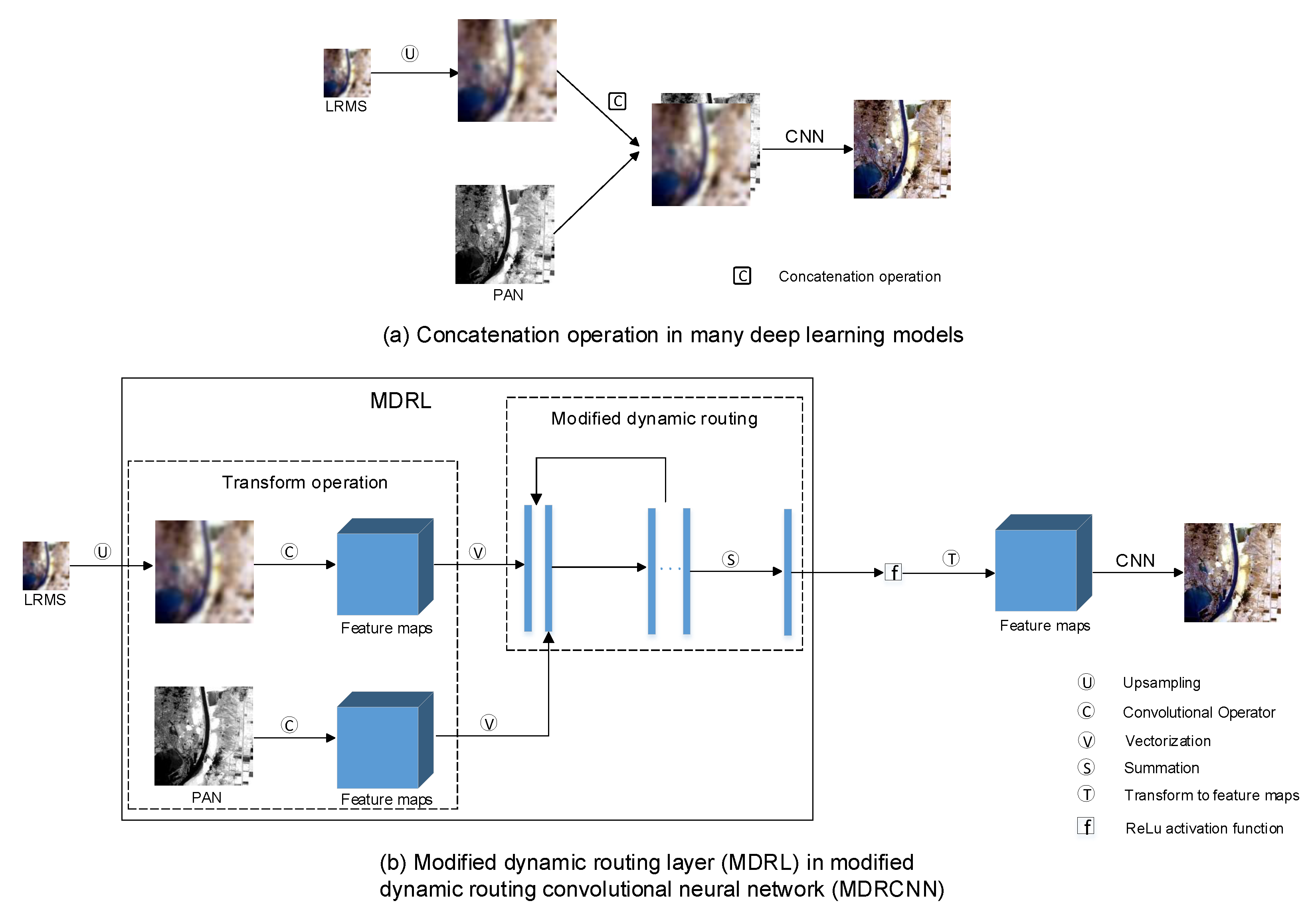
• To replace addition or concatenation operations in many deep learning models, we modify the dynamic routing algorithm to construct a modified dynamic routing layer (MDRL), where MDRL may be the first try to fuse LRMS images and PAN images by modifying the information transmission mode of capsules for pan-sharpening. In addition, the addition and concatenation operations are illustrated as special cases of our MDRL.
• In MDRL, the spatial location information is preserved in our model based on the convolutional operator in transform operation and the vectorize operation. Furthermore, the coupling coefficients are learned by the MDR algorithm, which make MDRL fuse the information of PAN images and LRMS images more effectively than with a simple concatenation or summation operation.
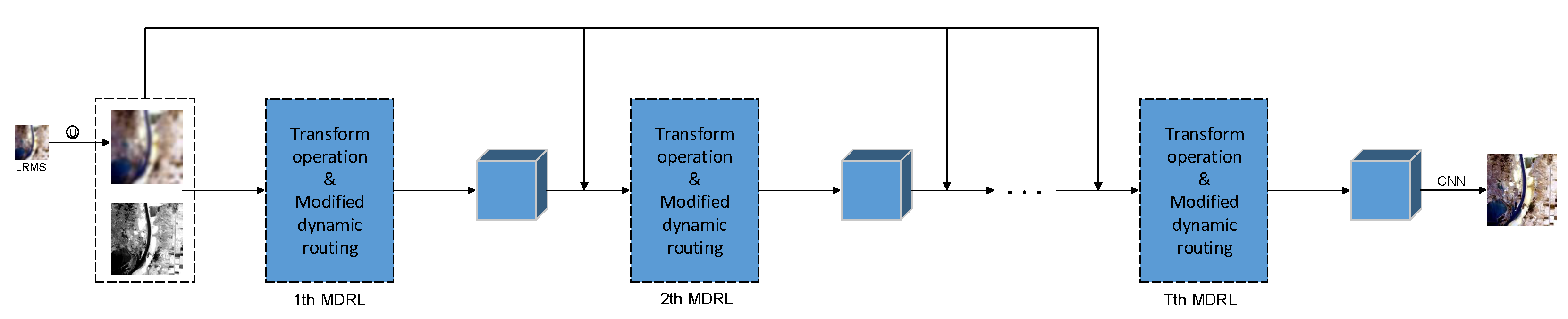
• Based on two baseline models (i.e., MIPSM and DRPNN), the proposed MDRL is inserted into them to generate our two neural networks named MDR–MIPSM and MDR–DRPNN. Quantitative experiments on three benchmark datasets demonstrate the superiority of our method.

The rest of this paper is organized as follows: MDRL and its corresponding models MDR–MIPSM and MDR–DRPNN are introduced in Section 2. Section 3 reports the experimental results. Section 4 mainly discusses our model by ablation experiments. Section 5 concludes this paper.

2. Materials and Methods

2.1. Dynamic Routing Algorithm

A dynamic routing algorithm is proposed to transfer information between capsules in adjacent layers of a capsule network [40,41]. Let us remark that the terminology “capsule” refers to the feature which is ready for classification or other high-level vision tasks. Capsules can be simply regarded as the feature maps. Let us assume ${\mathbf{u}}_i$ is a vector with m-dimension and it represents the output of the ith lower-level capsule. The “prediction vector” ${\widehat{\mathbf{u}}}_{j|i}$ of the jth higher-level capsule can be defined as multiplying a weight matrix ${\mathbf{W}}_{ij}\in {\mathbf{R}}^{n\times m}$ by ${\mathbf{u}}_i$:

$$\begin{array}{c}\hfill {\widehat{\mathbf{u}}}_{j|i}={\mathbf{W}}_{ij}\times {\mathbf{u}}_i.\end{array}$$

(1)

Thus, ${\widehat{\mathbf{u}}}_{j|i}$ is a n-dimension vector, and the capsule network sums all prediction ${\widehat{\mathbf{u}}}_{j|i}$ with weights $c_{ij}$ to obtain the input of the jth higher-level capsule ${\mathbf{s}}_j$ as follows:

$$\begin{array}{c}\hfill {\mathbf{s}}_j=\sum _{i=1}^M{c}_{ij}{\widehat{\mathbf{u}}}_{j|i},\end{array}$$

(2)

$$\begin{array}{c}\hfill c_{ij}=\frac{exp\left(b_{ij}\right)}{{\sum }_{k=1}^{N}exp\left(b_{ik}\right)},\end{array}$$

(3)

where $c_{ij}$ is the coupling coefficient between the ith lower-level capsule and the jth higher-level capsule, while M and N represent the number of lower-level capsules and higher-level capsules, respectively. $b_{ij}$ is the unnormalized coupling coefficient, which is iteratively updated by the dynamic routing algorithm and initialized to zero.

Instead of a traditional activation function, capsule networks propose a non-linear “squashing” function to handle ${\mathbf{s}}_j$ for generating its corresponding output ${\mathbf{v}}_j$. The “squashing” function is defined as

$$\begin{array}{c}\hfill {\mathbf{v}}_j=\frac{\parallel {\mathbf{s}}_j{\parallel }^2}{1+\parallel {\mathbf{s}}_j{\parallel }^2}\frac{{\mathbf{s}}_j}{\parallel {\mathbf{s}}_j\parallel }\end{array}$$

(4)

Then capsule networks calculate the agreement $a_{ij}$ between ${\mathbf{v}}_j$ and its prediction vector ${\widehat{\mathbf{u}}}_{j|i}$ as follows:

$$\begin{array}{c}\hfill a_{ij}={\mathbf{v}}_j\times {\widehat{\mathbf{u}}}_{j|i}\end{array}$$

(5)

Last, coupling coefficients $b_{ij}$ can be updated by adding $a_{ij}$. Supposing that there are r iterations, the final coupling coefficients $b_{ij}$ are fixed after r iterations. Now the outputs of higher-level capsules can be calculated by Equation (4). It is revealed that dynamic routing is an algorithm used for automatically modeling relationships between low-level and high-level capsules, where the coupling coefficient stands for which low-level capsule contributes more to the high-level capsule. As a matter of fact, this procedure can be applied to the fusion of information from LRMS and PAN images. That is to say, LRMS and PAN images are viewed as low-level capsules, while the fused image is the high-level capsule. In this manner, the dynamic routing algorithm can be viewed as a fusion strategy that automatically selects important features to reconstruct an HRMS image, where the importance is measured by the coupling coefficient. It is worth noting that coupling coefficients are determined by input data, which means that they can vary with the different samples. Thus, in the test stage, MDRL can perform better than the simple fusion strategy (e.g., addition or concatenation). Based on the original dynamic routing algorithm proposed in [40,41] designed for image classification, we modify it to make it compatible with pan-sharpening.

2.2. MDRL and MDRCNN

Here, for fusing the features of LRMS images and PAN images, a modified dynamic routing (MDR) algorithm and a modified dynamic routing layer (MDRL) are first introduced. Then, a deep model named modified dynamic routing CNN (MDRCNN) is proposed, based on MDRL.

For convenience, some notations should be summarized first. An LRMS image is denoted as $L\in {\mathbf{R}}^{h\times w\times B}$, where h, w and B are the height, width and band number, respectively. A similar notation is applied to a PAN image $P\in {\mathbf{R}}^{H\times W\times b}$. Thus, the size of our target HRMS image is $H\in {\mathbf{R}}^{H\times W\times B}$. In addition, the convolutional operator $Conv(X,c^{in},c^{out})$ is defined, where X, $c^{in}$ and $c^{out}$ represent the input feature, the number of input channels and the number of output channels, respectively.

Modifying the dynamic routing, MDRL is constructed for fusing the LRMS images and PAN images. The proposed MDRL consists of two parts: transform operation and modified dynamic routing (MDR) algorithm. Using the transform operation, we obtain the “prediction vector” of higher-level capsules. Then, MDR is proposed to obtain the representation of higher-level capsules which contains the information of LRMS images and PAN images.

(1) Transform operation: First, the input patch of LRMS images $L_p$ and the input patch of PAN images $P_p$ in the same area are taken as two lower-level capsules. Furthermore, suppose the size of $L_p$ is $h_1\times w_1\times B$ and the size of $P_p$ is $h_2\times w_2\times b$. Then, the up-sampling is used to handle $L_p$ to generate $L_u$ with the same spatial resolution of $P_p$ (i.e., $h_2\times w_2\times B$). Different from using multilayer perception in capsule networks, the convolutional operator in transform operation is adopted to use fewer parameters. Therefore, the prediction vector ${\widehat{\mathbf{u}}}_{j|i}\in {\mathbf{R}}^{h_2\times w_2\times c^{out}}$ can be expressed as

$$\begin{array}{c}\hfill {\widehat{\mathbf{u}}}_{j|1}=Conv(L_u,B,c^{out}),{\widehat{\mathbf{u}}}_{j|2}=Conv(P_p,b,c^{out}),\end{array}$$

(6)

where b is one, which means PAN images have only one band, and $c^{out}$ is usually set as $B+b$ (i.e., $c^{out}=B+1$). In other words, ${\widehat{\mathbf{u}}}_{j|1}$ and ${\widehat{\mathbf{u}}}_{j|2}$ are the feature maps of LRMS and PAN images, respectively. Last, for compatibility with MDR, ${\widehat{\mathbf{u}}}_{j|1}$ and ${\widehat{\mathbf{u}}}_{j|2}$ are vectorized to obtain two new prediction vectors ${\widehat{\mathbf{u}}}_{j|1}^c\in {\mathbf{R}}^{h_2{w}_2{c}^{out}\times 1}$ and ${\widehat{\mathbf{u}}}_{j|2}^c\in {\mathbf{R}}^{h_2{w}_2{c}^{out}\times 1}$ as the input of MDR.

(2) Modified dynamic routing (MDR) algorithm: The dynamic routing algorithm is used to transfer information between capsules in adjacent layers in the original capsule network. However, the capsule network with the original dynamic routing algorithm mainly handles the image classification, and it is not easy to apply image fusion. Thus, the dynamic routing algorithm needs to be modified to fit the pan-sharpening. Our modified dynamic routing algorithm has four major differences, compared to the dynamic routing algorithm in the capsule network. First, we delete the exponential function in Equation (3) due to the significant difference of ${\widehat{\mathbf{u}}}_{j|i}·{\mathbf{s}}_j$. In other words, if two values differ greatly, then an exponential function will further amplify the difference, which is very easy to cause $b_{ij}$ to be either 1 or 0. This evidently stands on the opposite of fusing the information of LRMS images and PAN images. Second, a lower-level capsule is coupled to all higher-level capsules in the original routing algorithm. In contrast to that, we make $c_{ij}$ to represent the importance of each lower-level capsule to higher-level capsules. Based on the above two changes, Equation (3) is modified as follows:

$$\begin{array}{c}\hfill c_{ij}=\frac{b_{ij}}{{\sum }_{k=1}^M{b}_{kj}},\end{array}$$

(7)

where M represents the number of lower-level capsules. Third, the “squashing” function is replaced by the classical activation function. At last, for easy calculation, the number of higher-level capsules N is set to 1. The specific MDR algorithm is shown in Algorithm 1.

Algorithm 1 MDR for pan-sharpening.

Input: Prediction vectors: ${\widehat{\mathbf{u}}}_{j|i}^c\in {\mathbf{R}}^{h_2{w}_2{c}^{out}}$. The number of iterations: r. The number of capsules in layer l: M. The number of capsules in layer (l + 1): N. Initialization: Initialize all capsules i in layer l and capsules j in layer (l + 1): $b_{ij}=$ 0. For r iterations do     for all capsules i in layer l and capsules j in layer (l + 1): use Equation (7) to obtain ${\mathbf{c}}_{ij}$.     for all capsules j in layer (l + 1): use Equation (2) to obtain ${\mathbf{s}}_j$.     for all capsules i in layer l and capsules j in layer (l + 1): $b_{ij}\leftarrow b_{ij}+{\widehat{\mathbf{u}}}_{j|i}\times {\mathbf{s}}_j$. End for For all capsules j in layer (l + 1): ${\mathbf{v}}_j=$ ReLU(${\mathbf{s}}_j$). output: ${\mathbf{v}}_j$.

As a plug-and-play module, MDRL can be plugged into a CNN to replace the addition or concatenation operation. As shown in Figure 1a, taking the concatenation operation as an example, many deep learning models directly concatenate the LMRS images and PAN images in channel dimension, which means that the PAN images equal the one channel of LRMS images. Plugging the MDRL, the modified dynamic routing convolutional neural network (MDRCNN) is proposed for pan-sharpening. In our MDRCNN, as shown in Figure 1b, the LMRS images and PAN images are treated as two lower-level capsules. Then, the transform operation and modified dynamic routing algorithm handle them and obtain the higher-level capsules to represent the fusion of LMRS images and PAN images. Last, the highest-level capsule is transmitted to the remaining network layers to generate the HRMS images for pan-sharpening.

In addition, the proposed MDRL can be stacked to plug in the MDRCNN. As shown in Figure 2, there are T MDRLs in the MDRCNN. Using the LRMS images and PAN images as input, the first fusion feature (i.e., higher-level capsule of the first MDRL) is obtained, via the first MDRL. Inspired by the deep residual network [43], taking the first fusion feature, LRMS images and PAN images as new lower-level capsules, the second MDRL can obtain the second fusion feature. By that analogy, MDRCNN with T MDRLs can be constructed for fusing the LRMS images and PAN images effectively.

2.3. The Relationship between the MDRL and Addition or Concatenation Operations

In this part, the relationship between the MDRL and summation or concatenation operations are analyzed. Through analysis, it is found that concatenation or addition operations are the special cases of the proposed MDRL when an affine transform and modified dynamic routing algorithm coordinate with each other.

Taking the concatenation as an example, concatenation operation means that many deep learning methods directly concatenate the PAN images and LRMS images into a channel dimension. Assuming that the size of the PAN images’ patch is $m\times n\times 1$, the size of the LRMS images’ patch is $m\times n\times c$ after up-sampling, and there is only one higher-level capsule. In our MDRL, the size of the filter for LRMS images $k^L$ is set to $3\times 3\times c$, and there are $(c+1)$ filters (i.e., $k_1^L,k_2^L,...,k_{c+1}^L$). Similarly, the size of the filter for PANs $k^P$ is set to $3\times 3\times 1$, and there are $(c+1)$ filters (i.e., $k_1^P,k_2^P,...,k_{c+1}^P$). Now, the prediction vector’s size is $mn(c+1)\times 1$. Based on Equation (7), suppose the coupling coefficient corresponding to LRMS images $C_{11}$ is $a(0<a<1)$; then, the coupling coefficient corresponding to PAN images $C_{21}$ is $1-a$. Every LRMS filter $k_i^L\in {\mathbf{R}}^{3\times 3\times c},i=1,...,c+1$ can be split into c channel filter $k_{ij}^L\in {\mathbf{R}}^{3\times 3},j=1,...,c$ and one channel filter’s size is $3\times 3$, which means $k_i^L=[k_{i1}^L,k_{i2}^L,...,k_{ic}^L,],i=1,...,c+1$. Then, we set the special value of the LRMS filters as follows:

$$k_{ij}^L=\left[\begin{array}{ccc}0& 0& 0\\ 0& 1/a& 0\\ 0& 0& 0\end{array}\right],ifi=jandi=1,...,c;k_{ii}^L=\left[\begin{array}{ccc}0& 0& 0\\ 0& 0& 0\\ 0& 0& 0\end{array}\right],ifi\ne jori=c+1.$$

Similarly, the PAN filters can be expressed as $k_i^P=\left[k_{i1}^P\right],k_{i1}^P\in {\mathbf{R}}^{3\times 3},i=1,...,c+1$. Then, we set the special value of the PAN filters as follows:

$$k_{i1}^P=\left[\begin{array}{ccc}0& 0& 0\\ 0& 1/(1-a)& 0\\ 0& 0& 0\end{array}\right],ifi=c+1;k_{i1}^L=\left[\begin{array}{ccc}0& 0& 0\\ 0& 0& 0\\ 0& 0& 0\end{array}\right],ifi=1,...,c.$$

Now, MDRL becomes the concatenation operation. It is easy to find that MDRL can also degenerate into the summation operation.

However, the filter weights for LRMS images and PAN images are obtained by the BP algorithm [44], and the coupling coefficients are learned by the MDR algorithm. Thus, the proposed MDRL can fuse the information of PAN images and LRMS images more effectively than a simple concatenation or summation operation.

2.4. Dataset and Evaluation Metrics

Here, three satellite datasets are chosen as our evaluation dataset, namely Landsat8, QuickBird and GaoFen2. Specifically, Landsat8 has 350 samples on its training dataset, 50 samples on its validation dataset and 100 samples on its test dataset. GaoFen2 has the same number of training/testing/validation images as Landsat8. QuickBird has 474/103/100 samples on its training/validation/test dataset. There are 10 bands of LRMS images on Landsat8, and the spatial up-scaling ratio (SUR) is set as 2. QuickBird and GaoFen2 contain 4 bands and the SUR is 4. Furthermore, all the samples are generated by using the Wald protocol [45].

Table 1. Summaries for datasets used for pan-sharpening.

Datasets	Training	Validation	Test	Bands	Spatial Up-Scaling Ratio (SUR)
QuickBird	474	103	100	4	4
Landsat8	350	50	100	10	2
GaoFen2	350	50	100	4	4

shows all the details of the three datasets above.

In the training process, the LRMS images are carved up into patches with a size of $32\times 32$; thus, the patches of PAN images have a size of (32*SUR)×(32*SUR). In the test phase, to measure performance of our method, we use the following four metrics: three spatial assessment metrics including structural similarity (SSIM) [46], error relative global dimensionless synthesis (ERGAS) [47], peak signal-to-noise ratio (PSNR) [48] and one spectral assessment metric spectral angle mapper (SAM) [49]. The fused image has a high quality when the PSNR and SSIM become higher, or the SAM and ERGAS become lower.

3. Experimental Results

In order to evaluate the effectiveness of our method, MDRL is plugged into two famous deep learning methods (i.e., MIPSM and DRPNN) to construct two new models named MDR–MIPSM and MDR–DRPNN. They are chosen because MIPSM uses addition operation and DRPNN uses concatenation operation to fuse LRMS images and PAN images. The proposed two models are compared with recent approaches on three benchmark datasets named Landsat8, QuickBird and GaoFen2. All the experiments are conducted on a computer with an NVIDIA RTX1080Ti GPU with 11 GB memory.

3.1. Comparison Methods and Training Details

In the experiments, we compare our two models, MDR–MIPSM and MDR–DRPNN, with some excellent methods, including seven traditional fusion methods and eight recent methods based on deep convolutional networks. Most of all, eight deep learning methods include two baseline models (i.e., MIPSM and DRPNN). Concretely, seven traditional fusion methods contain BDSD [23], Brovey [17], GS [18], HPF [50], IHS [19], Indusion [20] and SFIM [21]. A total of eight deep learning methods contain MIPSM [21], DRPNN [30], MSDCNN [31], RSIFNN [34], PANNET [51], CUNet [52], FGF-GAN [53], MHNet [54] and PMACNet [55].

Our MDR–MIPSM and MDR–DRPNN adopt $l_1$ loss as the loss function $\left|\right|H-\widehat{H}{\left|\right|}_1$, where H and $\widehat{H}$ represent the ground truth HRMS image and the reconstruction HRMS image, respectively. In most of our experiments, the configuration of MDR–MIPSM and MDR–DRPNN is set as follows: there are two MDRLs, the kernel size is set to $3\times 3$ and the number of modified dynamic routing’s iterations is set to 1 due to its ease of calculation. These two models are supervised by Adam [56] over 200 epochs, and the learning rate is set as $1\times {10}^{-3}$ with a 0.8 times decrease every 20 epochs. In addition, two layers of MIPSM and DRPNN are deleted to construct our MDR–MIPSM and MDR–DRPNN, due to the number of MDRL being 2 in our experiments.

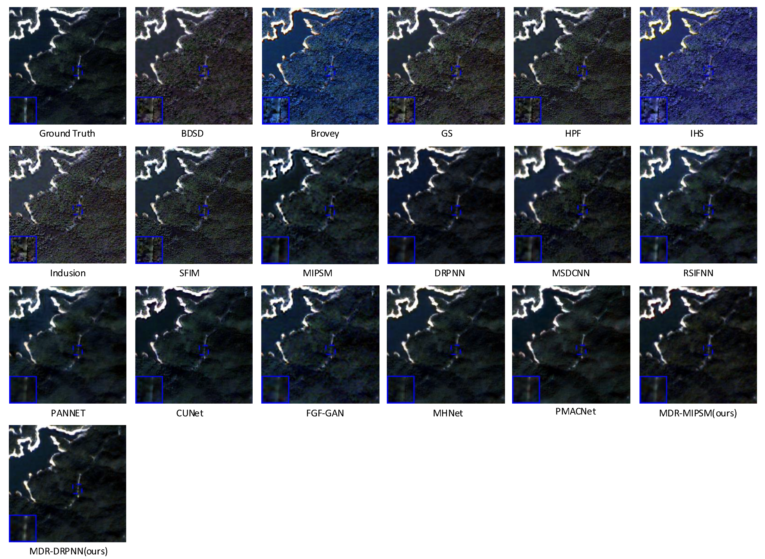
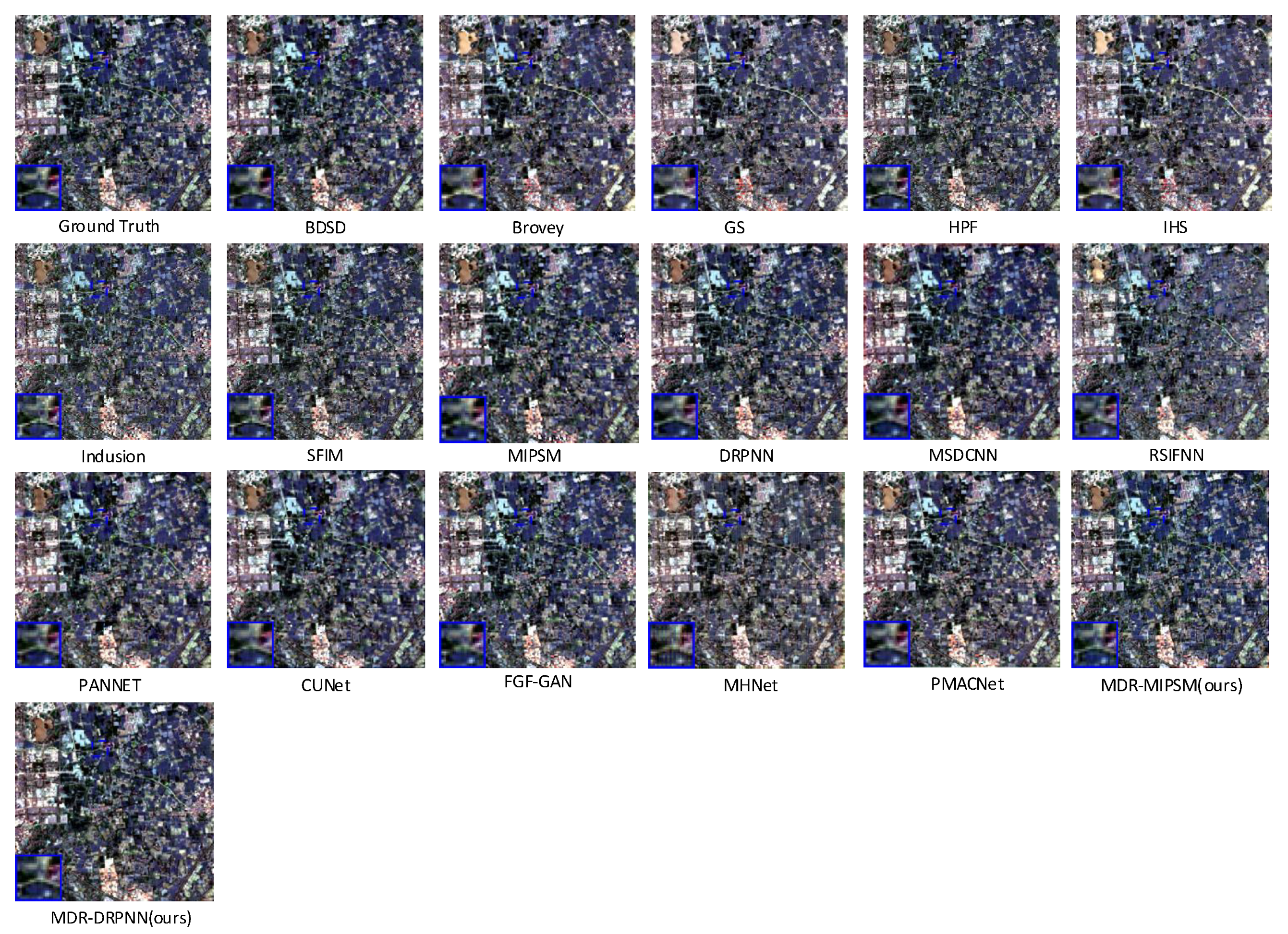
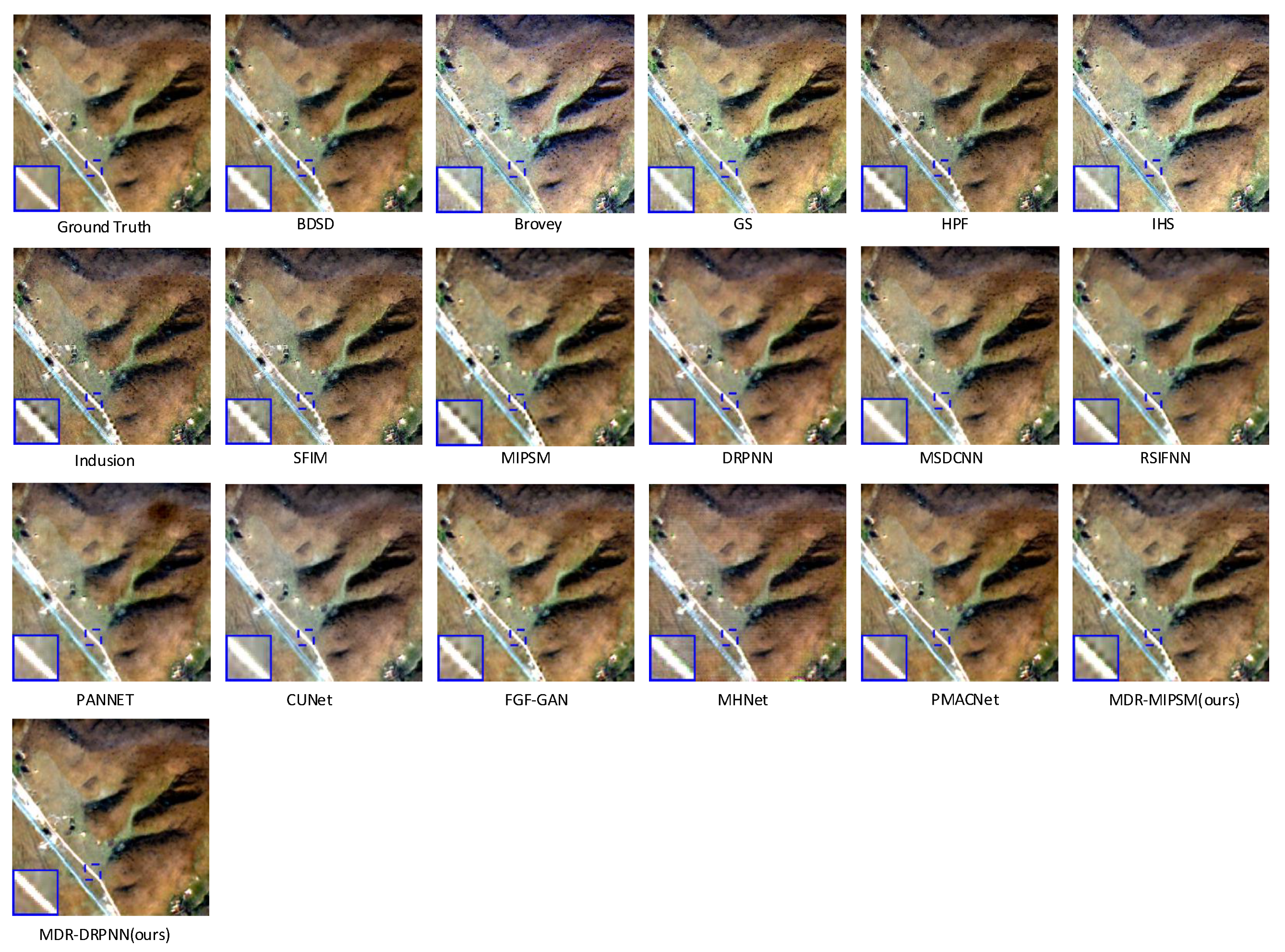
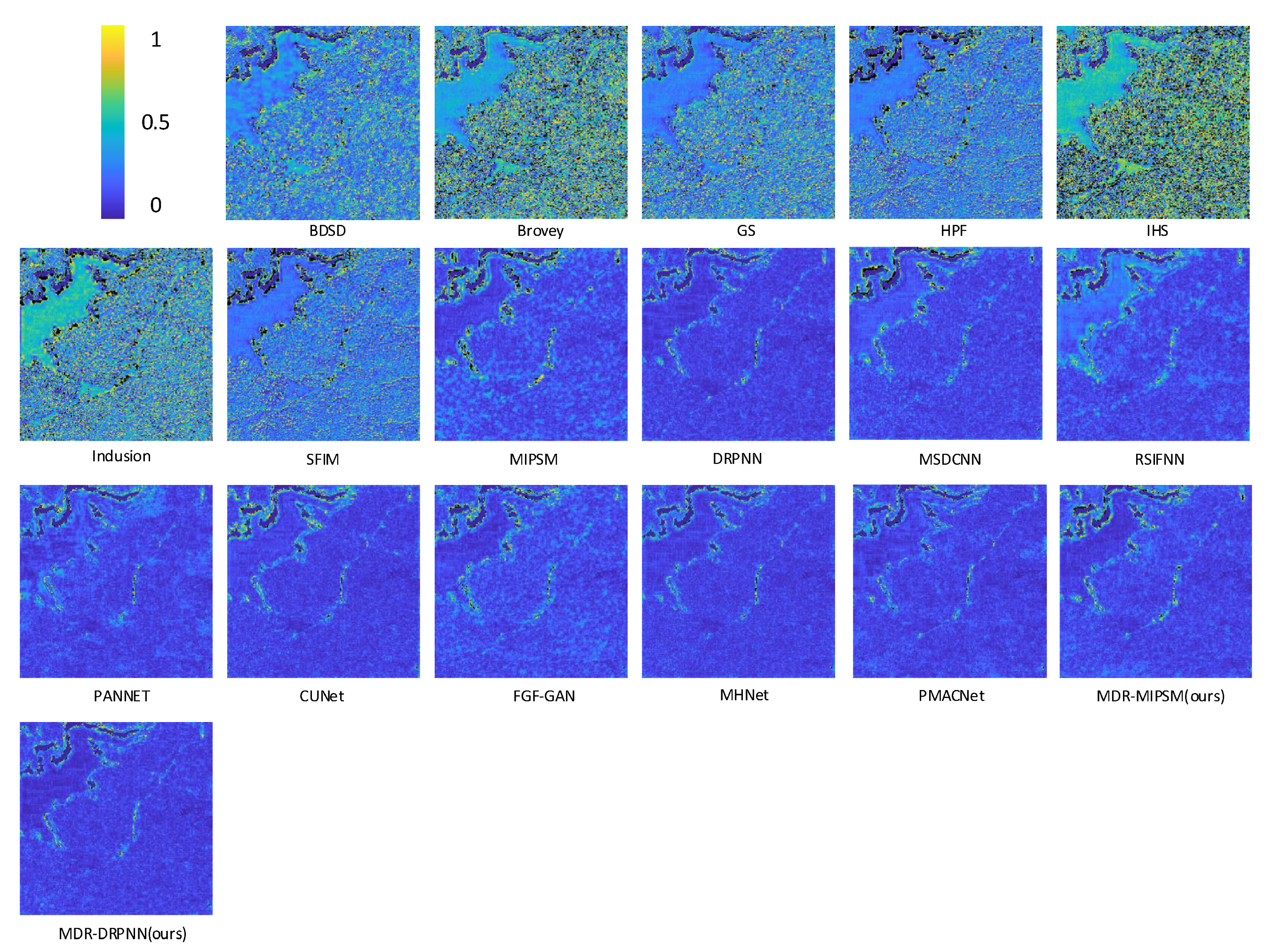
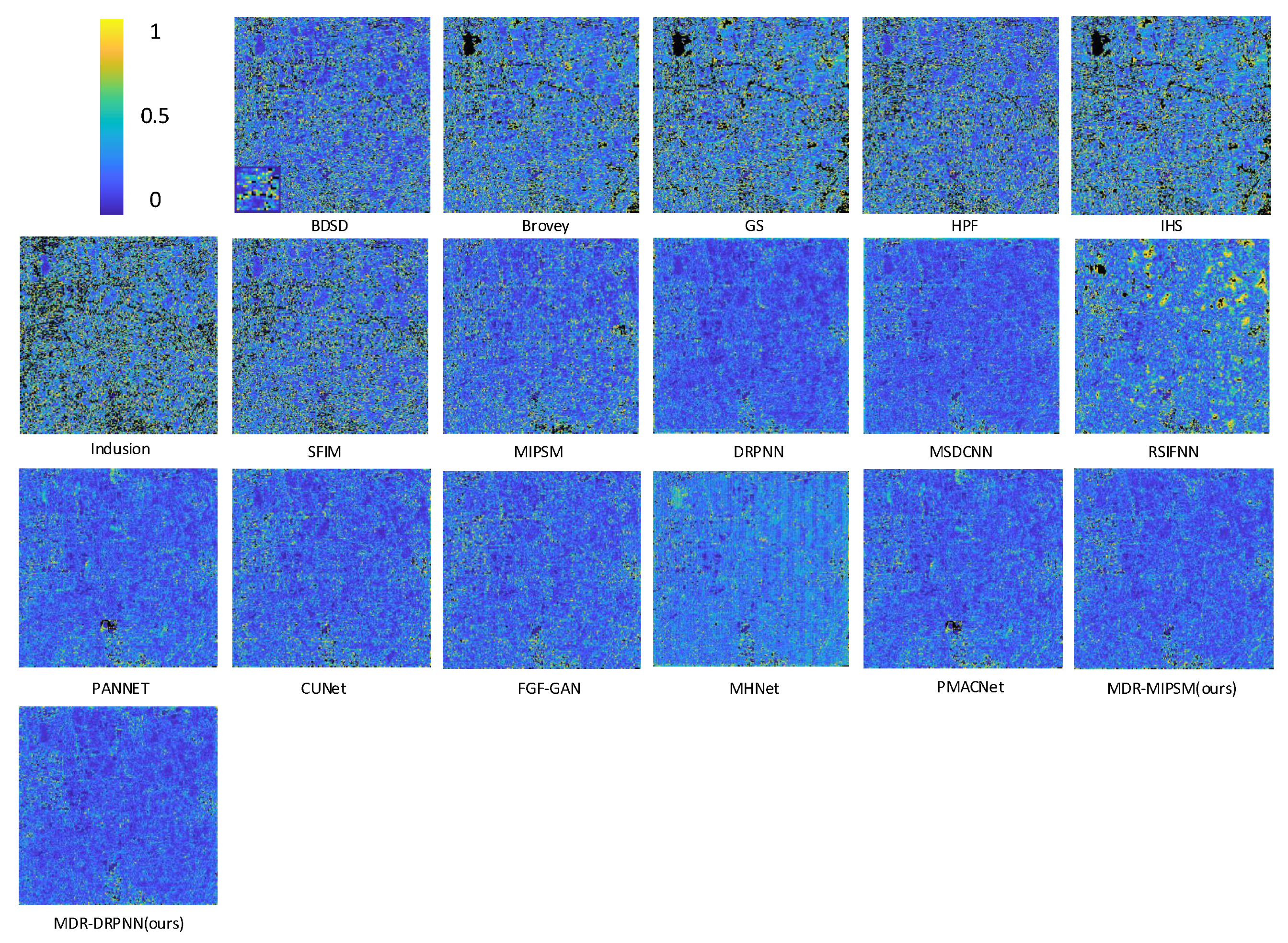
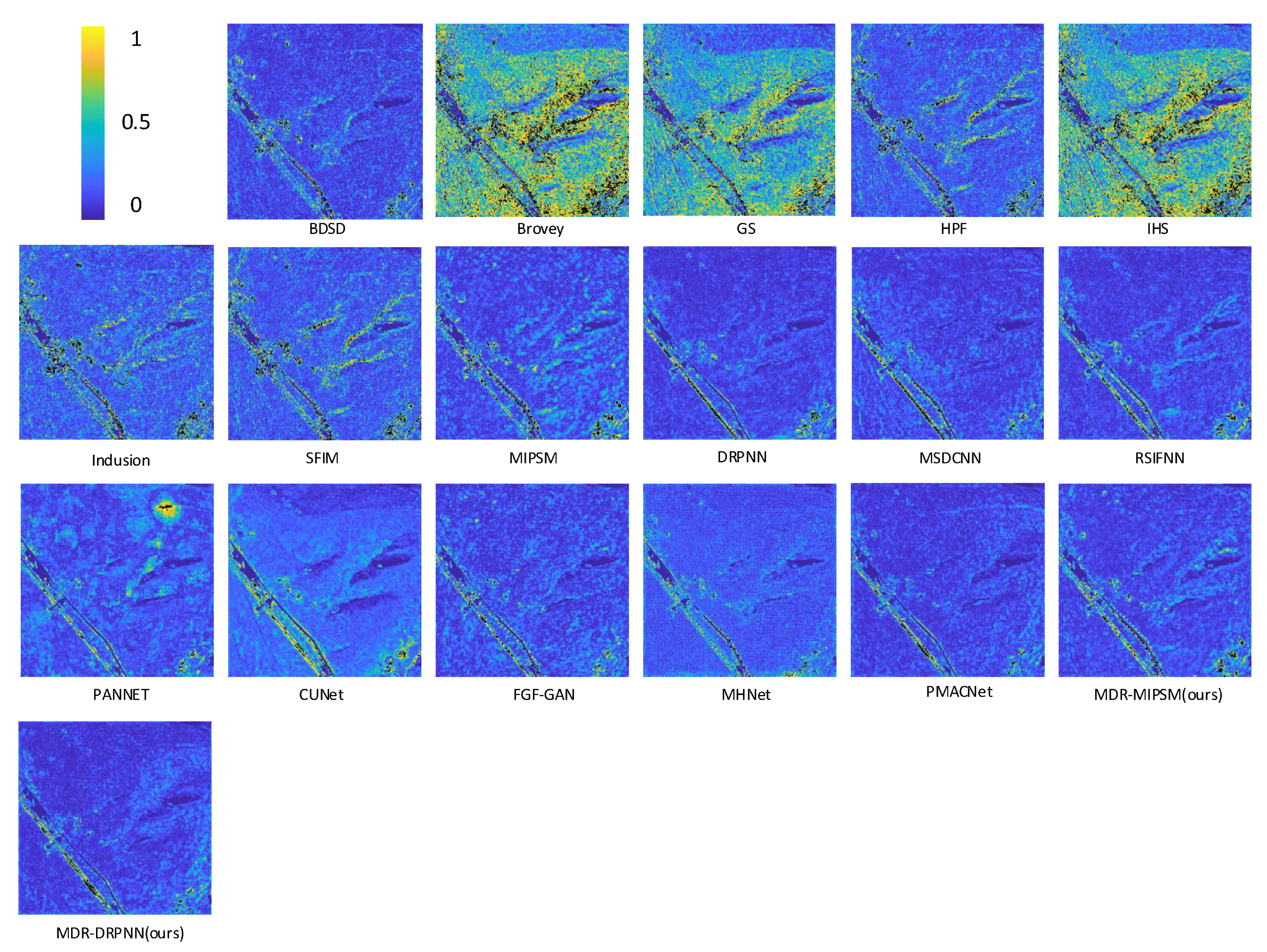
3.2. Performance Comparison

Table 2. Comparison results on QuickBird dataset. The best and the second best are highlighted by bold and underlined, respectively. The up or down arrow indicates higher or lower metric corresponding to better images.

Method	PSNR ↑	SSIM ↑	SAM ↓	ERGAS ↓
BDSD [23]	23.5540	0.7156	0.0765	4.8874
Brovey [17]	25.2744	0.7370	0.0640	4.2085
GS [18]	26.0305	0.6829	0.0586	3.9498
HPF [50]	25.9977	0.7378	0.0588	3.9452
IHS [19]	24.3826	0.6742	0.0647	4.6208
Indusion [20]	25.7623	0.6377	0.0674	4.2514
SFIM [21]	24.0351	0.6409	0.0739	4.8282
MIPSM [21]	27.7323	0.8411	0.0522	3.1550
DRPNN [30]	31.0415	0.8993	0.0378	2.2250
MSDCNN [31]	30.1245	0.8728	0.0434	2.5649
RSIFNN [34]	30.5769	0.8898	0.0405	2.3530
PANNET [51]	30.9631	0.8988	0.0368	2.2648
CUNet [52]	30.3612	0.8876	0.0428	2.4178
FGF-GAN [53]	30.3465	0.8761	0.0407	2.4103
MHNet [54]	31.1557	0.8947	0.0368	2.1931
PMACNet [55]	31.0974	0.9020	0.0384	2.3141
MDR–MIPSM (ours)	29.8426	0.8837	0.0431	2.6694
MDR–DRPNN (ours)	31.4626	0.9038	0.0358	2.1348

shows the quantitative results of our methods, compared with all comparison methods on the QuickBird dataset. The proposed MDR–MIPSM and MDR–DRPNN are superior to the traditional pan-sharpening approaches. In the deep learning methods, our MDR–DRPNN also achieves the best performance on all four indicators. Moreover, our MDR–MIPSM and MDR–DRPNN perform visibly better than MIPSM and DRPNN. Specifically, the result obtained by our MDR–MIPSM exceeds MIPSM in PSNR by almost 2.1 db, which is a significant improvement.

In

Table 3. Comparison results on Landsat8 dataset. The best and the second best are highlighted by bold and underlined, respectively. The up or down arrow indicates higher or lower metric corresponding to better images.

Method	PSNR ↑	SSIM ↑	SAM ↓	ERGAS ↓
BDSD [23]	33.8065	0.9128	0.0255	1.9128
Brovey [17]	32.4030	0.8533	0.0206	1.9806
GS [18]	32.0163	0.8687	0.0304	2.2119
HPF [50]	32.6691	0.8712	0.0250	2.0669
IHS [19]	32.8772	0.8615	0.0245	2.3128
Indusion [20]	30.8476	0.8168	0.0359	2.4216
SFIM [21]	32.7207	0.8714	0.0248	2.0775
MIPSM [21]	35.4891	0.9389	0.0209	1.5769
DRPNN [30]	37.3639	0.9613	0.0173	1.3303
MSDCNN [31]	36.2536	0.9581	0.0176	1.4160
RSIFNN [34]	37.0782	0.9547	0.0172	1.3273
PANNET [51]	38.0910	0.9647	0.0152	1.3021
CUNet [52]	37.0468	0.9610	0.0179	1.3430
FGF-GAN [53]	38.0832	0.9533	0.0165	1.2714
MHNet [54]	37.0049	0.9566	0.0189	1.3509
PMACNet [55]	38.3271	0.9670	0.0158	1.2278
MDR–MIPSM (ours)	37.3317	0.9614	0.0171	1.4071
MDR–DRPNN (ours)	38.5876	0.9685	0.0153	1.2012

and

Table 4. Comparison results on GaoFen2 dataset. The best and the second best are highlighted by bold and underlined, respectively. The up or down arrow indicates higher or lower metric corresponding to better images.

Method	PSNR ↑	SSIM ↑	SAM ↓	ERGAS ↓
BDSD [23]	30.2114	0.8732	0.0126	2.3963
Brovey [17]	31.5901	0.9033	0.0110	2.2088
GS [18]	30.4357	0.8836	0.0101	2.3075
HPF [50]	30.4812	0.8848	0.0113	2.3311
IHS [19]	30.4754	0.8639	0.0108	2.3546
Indusion [20]	30.5359	0.8849	0.0113	2.3457
SFIM [21]	30.4021	0.8501	0.0129	2.3688
MIPSM [21]	32.1761	0.9392	0.0104	1.8830
DRPNN [30]	35.1182	0.9663	0.0098	1.3078
MSDCNN [31]	33.6715	0.9685	0.0090	1.4720
RSIFNN [34]	33.0588	0.9588	0.0112	1.5658
PANNET [51]	34.5774	0.9635	0.0089	1.4750
CUNet [52]	33.6919	0.9630	0.0184	1.5839
FGF-GAN [53]	35.0450	0.9449	0.0089	1.4351
MHNet [54]	33.8930	0.9291	0.0176	1.3697
PMACNet [55]	35.3506	0.9678	0.0101	1.2658
MDR–MIPSM (ours)	34.2735	0.9530	0.0105	1.5150
MDR–DRPNN (ours)	35.6512	0.9704	0.0091	1.2177

, our MDR–MIPSM and MDR–DRPNN are compared with other state-of-the-art methods on the Landsat8 and GaoFen2 datasets. It is found that our MDR–DRPNN performs slightly worse than PANNet on the SAM indicator, and visibly better than DRPNN on all metrics on Table 3. In addition, FGF-GAN and PANNet perform slightly better than our MDR–DRPNN on the SAM indicator in Table 4. However, on PSNR, SSIM and ERGAS, our MDR–DRPNN achieves the best performance, compared with all other models.

Moreover, we display a visual comparison of our models with other methods on three datasets, as shown in Figure 3, Figure 4 and Figure 5. Compared with other methods, our MDR–DRPNN not only preserves the spectral information of the LRMS images, but also has a wealth of detailed information contained in the PAN images. From the amplified area, we can see that our MDR–DRPNN generates high-quality HRMS images, which avoids spatial and spectral distortion effectively. In addition, taking the ground truth image (upper left corner of Figure 3, Figure 4 and Figure 5) as a reference, we show the corresponding residual map to evaluate the quality of images generated by our MDR–MIPSM and MDR–DRPNN in Figure 6, Figure 7 and Figure 8. From the residual map, we find that the fused images of our MDR–DRPNN are the closest to the ground truth, which demonstrates the effectiveness of our methods.

By comparing the results between three datasets, a careful analysis of our model is conducted. It is found that the spatial location information is preserved in our model based on the convolutional operator in transform operation and the vectorize operation. Thus, our model can extract more spatial detail information, which is consistent with the experimental results. By examining the image of the three datasets, the Landsat8 dataset contains more buildings, which means it offers offer a wealth of spatial detailed information compared to the QuickBird and GaoFen2 datasets. Taking the base model DRPNN [30] as example, our model MDR–DRPNN significantly improves 1.2237 db on the PSNR of Landsat8, while it improves 0.4211 db and 0.5330 db on the PSNR of the QuickBird and GaoFen2 datasets, respectively. Furthermore, this reminds us that our future study should pay more attention to extract spectral detail information.

In addition, the real HRLS image is not accessible in reality. Thus, pan-sharpening in a real LRMS image and PAN image (i.e., full scale experiment) comes with reference-free image quality metrics. Here, Quality with No Reference (QNR), spectral distortion index ($D_{\lambda }$) and spatial distortion index ($D_S$) are chosen to evaluate the pan-sharpening quality of a full image on the Landsat8 and QuickBird datasets. The specific experimental results are shown in the following

Table 5. Quantitative results for the Landsat8 and QuickBird datasets at full scale. The best and the second best are highlighted by bold and underlined, respectively. The up or down arrow indicates higher or lower metric corresponding to better images.

	Landsat8			QuickBird
Method	QNR↑	${\mathit{D}}_{\mathit{\lambda }}$↓	${\mathit{D}}_{\mathit{S}}$↓	QNR↑	${\mathit{D}}_{\mathit{\lambda }}$↓	${\mathit{D}}_{\mathit{S}}$↓
BDSD	0.7632	0.1064	0.1469	0.6061	0.1660	0.2741
GS	0.8195	0.0580	0.1310	0.7134	0.0937	0.2157
HPF	0.8764	0.0475	0.0801	0.7626	0.1062	0.1484
IHS	0.7381	0.1360	0.1470	0.5547	0.1975	0.3095
Indusion	0.9239	0.0235	0.0539	0.8104	0.1083	0.0923
SFIM	0.8865	0.0464	0.0706	0.7573	0.1062	0.1544
CUNet	0.9132	0.0265	0.0621	0.7864	0.1367	0.0894
RSIFNN	0.9273	0.0278	0.0468	0.7709	0.1064	0.1392
MHNet	0.9117	0.0373	0.0535	0.8408	0.0760	0.0902
MSDCNN	0.9380	0.0237	0.0392	0.7419	0.1246	0.1557
PANNET	0.9499	0.0214	0.0293	0.8383	0.0865	0.0824
MIPSM	0.9273	0.0172	0.0566	0.7850	0.1290	0.0998
DRPNN	0.9380	0.0252	0.0378	0.7999	0.1087	0.1025
MDR–MIPSM (ours)	0.9354	0.0192	0.0471	0.7939	0.1028	0.1167
MDR–DRPNN (ours)	0.9500	0.0170	0.0339	0.8469	0.0680	0.0916

. As shown in this table, our model MDR–DRPNN obtains excellent experimental results on three metrics and two datasets, which is competitive with other deep learning models. In particular, compared to the base model DRPNN, our model MDR–DRPNN improves by 0.012 and 0.047 on the QNR of the Landsat8 and QuickBird datasets, respectively. Furthermore, MDR–MIPSM increases the values on the QNR metric with the base model MIPSM. Another two metrics $D_{\lambda }$ and $D_S$ also show the same improvement. Thus, the proposed plug-and-play MDRL is helpful to fuse the LRMS image and PAN image.

4. Discussion

In section, we use MDR–DRPNN as backbone and conduct some ablation experiments to further verify the efficiency of our methods. We discussed the influence of the number of MDRL, the number of iterations in MDR and the parameter numbers of MDR–DRPNN, because they all play important roles in MDR–DRPNN.

4.1. Influence of the Number of MDRL

The depth of MDR–DRPNN depends on the number of MDRL; thus, it should be first to discuss. As shown in

Table 6. The influence of the number of MDRL, based on MDR–DRPNN and Quickbird dataset. It is worth noting that #MDRL represents the number of MDRL.

#MDRL	PSNR ↑	SSIM ↑	SAM ↓	ERGAS ↓
1	31.4074	0.9022	0.0354	2.1382
2	31.4626	0.9038	0.0358	2.1348
3	31.3480	0.9029	0.0358	2.1617

, the number of MDRL is set as 1, 2 and 3, respectively. Taking the PSNR, SSIM, SAM and ERGAS as metrics, the MDR–DRPNN model and Quickbird dataset are used to evaluate it. From this table, it is found that most of the metrics increase slightly and then decrease, when the number of MDRL increases from 1 to 2 to 3. Thus, the number of MDRL is set as 2 in our experiments.

4.2. Influence of the Number of Iterations in MDR

In this section, the influence of the number of iterations on MDR is studied, due to the fact that it is the most important parameter in MDR. For easy calculation, the number of higher-level capsules is set as 1 in this experiment.

Table 7. The influence of the number of iterations in modified dynamic routing, based on MDR–DRPNN and Quickbird dataset. It is worth noting that #Iterations represents the number of iterations in modified dynamic routing.

#Iterations	PSNR ↑	SSIM ↑	SAM ↓	ERGAS ↓
1	31.4626	0.9038	0.0358	2.1348
2	31.4435	0.9036	0.0362	2.1193
3	31.3661	0.9049	0.0353	2.1509

shows the results on the Quickbird dataset, based on the MDR–DRPNN model and PSNR, SSIM, SAM and ERGAS metrics. From this table, it is found that no matter the number of iterations, our proposed MDR–DRPNN’s performance does not vary much. This also verifies the stability of our model. Thus, for the purpose of saving training and testing time, the number of iterations is set as 1 in our most experiments.

4.3. Parameter Numbers

In our method, the MDRL is used to replace the addition or concatenation operations. Thus, based on the Quickbird dataset, the parameters of our MDR–MIPSM and MDR–DRPNN are analyzed here. As said in the training details, two layers of MIPSM and DRPNN are deleted to construct our models MDR–MIPSM and MDR–DRPNN, due to the number of MDRL being 2 in our experiments. As shown in

Table 8. The number of parameters of our MDR–MIPSM and MDR–DRPNN, compared with MIPSM and DRPNN, based on Quickbird dataset.

Method	MIPSM	MDR–MIPSM	DRPNN	MDR–DRPNN
#Parameters (million)	87,047	68,551	375,293	302,595
PSNR	27.7323	29.8426	31.0415	31.4626

, it is found that the amount of parameters of our models decreases visibly more than MIPSM and DRPNN, but our models achieve better results.

This may be due the fact to that our network can perform more efficient fusion and achieve a reasonable balance between spectral and spatial information, which proves the efficacy of our method.

5. Conclusions

In this study, due to the fact that the addition and concatenation operations may cause loss of information, we design a modified dynamic routing layer (MDRL) to replace them for pan-sharpening, via a modified dynamic routing (MDR) algorithm. Based on the convolutional operator in transform operation and the vectorize operation, our MDRL can preserve more spatial location information. In addition, the coupling coefficient in MDRL can vary with the input samples, which make MDRL fuse the PAN and LRMS images in the test stage effectively. Using MDRL, two deep models named MDR–MIPSM and MDR–DRPNN are proposed, and extensive experimental results on benchmark pan-sharpening datasets demonstrate the efficacy of our method, compared with other excellent models. In the future work, we will pay more attention to extract spectral detail information, which may be implemented by the attention mechanism.

References

1. Cao, X.; Zhou, F.; Xu, L.; Meng, D.; Xu, Z.; Paisley, J. Hyperspectral image classification with markov random fields and a convolutional neural network. IEEE Trans. Image Process. 2018, 27, 2354–2367. [Google Scholar] [CrossRef] [PubMed]
2. Cao, X.; Yao, J.; Xu, Z.; Meng, D. Hyperspectral image classification with convolutional neural network and active learning. IEEE Trans. Geosci. Remote Sens. 2020, 58, 4604–4616. [Google Scholar] [CrossRef]
3. Cao, X.; Fu, X.; Xu, C.; Meng, D. Deep spatial-spectral global reasoning network for hyperspectral image denoising. IEEE Trans. Geosci. Remote Sens. 2021, 60, 5504714. [Google Scholar] [CrossRef]
4. Hong, D.; Gao, L.; Yao, J.; Zhang, B.; Plaza, A.; Chanussot, J. Graph convolutional networks for hyperspectral image classification. IEEE Trans. Geosci. Remote Sens. 2020, 59, 5966–5978. [Google Scholar] [CrossRef]
5. Hong, D.; Gao, L.; Yokoya, N.; Yao, J.; Chanussot, J.; Du, Q.; Zhang, B. More diverse means better: Multimodal deep learning meets remote-sensing imagery classification. IEEE Trans. Geosci. Remote Sens. 2020, 59, 4340–4354. [Google Scholar] [CrossRef]
6. Wu, X.; Hong, D.; Chanussot, J. Convolutional neural networks for multimodal remote sensing data classification. IEEE Trans. Geosci. Remote Sens. 2022, 60, 5517010. [Google Scholar] [CrossRef]
7. Yao, J.; Cao, X.; Hong, D.; Wu, X.; Meng, D.; Chanussot, J.; Xu, Z. Semi-active convolutional neural networks for hyperspectral image classification. IEEE Trans. Geosci. Remote Sens. 2022, 60, 5537915. [Google Scholar] [CrossRef]
8. Hong, D.; Hu, J.; Yao, J.; Chanussot, J.; Zhu, X. Multimodal remote sensing benchmark datasets for land cover classification with a shared and specific feature learning model. ISPRS J. Photogramm. Remote Sens. 2021, 178, 68–80. [Google Scholar] [CrossRef]
9. Hong, D.; Han, Z.; Yao, J.; Gao, L.; Zhang, B.; Plaza, A.; Chanussot, J. Spectralformer: Rethinking hyperspectral image classification with transformers. IEEE Trans. Geosci. Remote Sens. 2022, 60, 5518615. [Google Scholar] [CrossRef]
10. Prades, J.; Safont, G.; Salazar, A.; Vergara, L. Estimation of the number of endmembers in hyperspectral images using agglomerative clustering. Remote Sens. 2020, 12, 3585. [Google Scholar] [CrossRef]
11. Zhu, X.; Yue, K.; Junmin, L. Estimation of the number of endmembers via thresholding ridge ratio criterion. IEEE Geosci. Remote Sens. Mag. 2019, 58, 637–649. [Google Scholar] [CrossRef]
12. Dhaini, M.; Berar, M.; Honeine, P.; Van Exem, A. End-to-End Convolutional Autoencoder for Nonlinear Hyperspectral Unmixing. Remote Sens. 2022, 14, 3341. [Google Scholar] [CrossRef]
13. Liu, J.; Yuan, S.; Zhu, X.; Huang, Y.; Zhao, Q. Nonnegative matrix factorization with entropy regularization for hyperspectral unmixing. Int. J. Remote Sens. 2021, 42, 6359–6390. [Google Scholar] [CrossRef]
14. Cao, X.; Fu, X.; Hong, D.; Xu, Z.; Meng, D. Pancsc-net: A model-driven deep unfolding method for pansharpening. IEEE Trans. Geosci. Remote Sens. 2021, 60, 5404713. [Google Scholar] [CrossRef]
15. Vivone, G.; Dalla Mura, M.; Garzelli, A.; Restaino, R.; Scarpa, G.; Ulfarsson, M.O.; Alparone, L.; Chanussot, J. A new benchmark based on recent advances in multispectral pansharpening: Revisiting pansharpening with classical and emerging pansharpening methods. IEEE Geosci. Remote Sens. Mag. 2020, 9, 53–81. [Google Scholar] [CrossRef]
16. Meng, X.; Shen, H.; Li, H.; Zhang, L.; Fu, R. Review of the pansharpening methods for remote sensing images based on the idea of meta-analysis: Practical discussion and challenges. Inf. Fusion 2019, 46, 102–113. [Google Scholar] [CrossRef]
17. Gillespie, A.R.; Kahle, A.B.; Walker, R.E. Color enhancement of highly correlated images. I. Decorrelation and HSI contrast stretches. Remote Sens. Environ. 1986, 20, 209–235. [Google Scholar] [CrossRef]
18. Laben, C.A.; Brower, B.V. Process for Enhancing the Spatial Resolution of Multispectral Imagery Using Pan-Sharpening. U.S. Patent 6,011,875, 4 January 2000. [Google Scholar]
19. Haydn, R. Application of the ihs color transform to the processing of multisensor data and image enhancement. In Proceedings of the International Symposium on Remote Sensing of Arid and Semi-Arid Lands, Cairo, Egypt, 19–25 January 1982. [Google Scholar]
20. Khan, M.M.; Chanussot, J.; Condat, L.; Montanvert, A. Indusion: Fusion of multispectral and panchromatic images using the induction scaling technique. IEEE Geosci. Remote Sens. Lett. 2008, 5, 98–102. [Google Scholar] [CrossRef]
21. Liu, J.G. Smoothing filter-based intensity modulation: A spectral preserve image fusion technique for improving spatial details. Int. J. Remote Sens. 2000, 21, 3461–3472. [Google Scholar] [CrossRef]
22. Otazu, X.; González-Audícana, M.; Fors, O.; Núñez, J. Introduction of sensor spectral response into image fusion methods. Application to wavelet-based methods. IEEE Trans. Geosci. Remote Sens. 2005, 43, 2376–2385. [Google Scholar] [CrossRef]
23. Garzelli, A.; Nencini, F.; Capobianco, L. Optimal mmse pan sharpening of very high resolution multispectral images. IEEE Trans. Geosci. Remote Sens. 2007, 46, 228–236. [Google Scholar] [CrossRef]
24. He, X.; Condat, L.; Bioucas-Dias, J.; Chanussot, J.; Xia, J. A new pansharpening method based on spatial and spectral sparsity priors. IEEE Trans. Image Process. 2014, 23, 4160–4174. [Google Scholar] [CrossRef] [PubMed]
25. Fang, F.; Li, F.; Shen, C.; Zhang, G. A variational approach for pan-sharpening. IEEE Trans. Image Process. 2013, 22, 2822–2834. [Google Scholar] [CrossRef] [PubMed]
26. Krizhevsky, A.; Sutskever, I.; Hinton, G.E. Imagenet classification with deep convolutional neural networks. Commun. ACM 2017, 60, 84–90. [Google Scholar] [CrossRef]
27. Simonyan, K.; Zisserman, A. Very deep convolutional networks for large-scale image recognition. arXiv 2014, arXiv:1409.1556. [Google Scholar]
28. Huang, G.; Liu, Z.; Van Der Maaten, L.; Weinberger, K.Q. Densely connected convolutional networks. In Proceedings of the IEEE Conference on Computer Vision and Pattern Recognition, Honolulu, HI, USA, 21 July 2017. [Google Scholar]
29. Masi, G.; Cozzolino, D.; Verdoliva, L.; Scarpa, G. Pansharpening by convolutional neural networks. Remote Sens. 2016, 8, 594. [Google Scholar] [CrossRef]
30. Wei, Y.; Yuan, Q.; Shen, H.; Zhang, L. Boosting the accuracy of multispectral image pansharpening by learning a deep residual network. IEEE Geosci. Remote Sens. Lett. 2017, 14, 1795–1799. [Google Scholar] [CrossRef]
31. Yuan, Q.; Wei, Y.; Meng, X.; Shen, H.; Zhang, L. A multiscale and multidepth convolutional neural network for remote sensing imagery pan-sharpening. IEEE J. Sel. Top. Appl. Earth Obs. Remote Sens. 2018, 11, 978–989. [Google Scholar] [CrossRef]
32. Xiong, Z.; Guo, Q.; Liu, M.; Li, A. Pan-sharpening based on convolutional neural network by using the loss function with no-reference. IEEE J. Sel. Top. Appl. Earth Obs. Remote Sens. 2020, 14, 897–906. [Google Scholar] [CrossRef]
33. Guo, Q.; Li, S.; Li, A. An Efficient Dual Spatial–Spectral Fusion Network. IEEE Trans. Geosci. Remote Sens. 2022, 60, 1–13. [Google Scholar] [CrossRef]
34. Shao, Z.; Cai, J. Remote sensing image fusion with deep convolutional neural network. IEEE J. Sel. Top. Appl. Earth Obs. Remote Sens. 2018, 11, 1656–1669. [Google Scholar] [CrossRef]
35. Liu, L.; Wang, J.; Zhang, E.; Li, B.; Zhu, X.; Zhang, Y.; Peng, J. Shallow–deep convolutional network and spectral-discrimination-based detail injection for multispectral imagery pan-sharpening. IEEE J. Sel. Top. Appl. Earth Obs. Remote Sens. 2020, 13, 1772–1783. [Google Scholar] [CrossRef]
36. Vivone, G.; Dalla Mura, M.; Garzelli, A.; Pacifici, F. A benchmarking protocol for pansharpening: Dataset, preprocessing, and quality assessment. IEEE J. Sel. Top. Appl. Earth Obs. Remote Sens. 2021, 14, 6102–6118. [Google Scholar] [CrossRef]
37. Jin, Z.; Zhuo, Y.; Zhang, T.; Jin, X.; Jing, S.; Deng, L. Remote sensing pansharpening by full-depth feature fusion. Remote Sens. 2022, 14, 466. [Google Scholar] [CrossRef]
38. Wang, W.; Zhou, Z.; Liu, H.; Xie, G. MSDRN: Pansharpening of multispectral images via multi-scale deep residual network. Remote Sens. 2021, 13, 1200. [Google Scholar] [CrossRef]
39. Zhang, E.; Fu, Y.; Wang, J.; Liu, L.; Yu, K.; Peng, J. Msac-net: 3d multi-scale attention convolutional network for multi-spectral imagery pansharpening. Remote Sens. 2022, 14, 2761. [Google Scholar] [CrossRef]
40. Sara, S.; Nicholas, F.; Geoffrey, E.H. Dynamic routing between capsules. In Proceedings of the Neural Information Processing Systems, Long Beach, CA, USA, 4 December 2017. [Google Scholar]
41. Hinton, G.E.; Sabour, S.; Frosst, N. Matrix capsules with em routing. In Proceedings of the International Conference on Learning Representations, Vancouver, BC, Canada, 30 April 2018. [Google Scholar]
42. Sun, K.; Zhang, J.; Liu, J.; Yu, R.; Song, Z. Drcnn: Dynamic routing convolutional neural network for multi-view 3d object recognition. IEEE Trans. Image Process. 2020, 30, 868–877. [Google Scholar] [CrossRef]
43. He, K.; Zhang, X.; Ren, S.; Sun, J. Deep residual learning for image recognition. In Proceedings of the IEEE Conference on Computer Vision and Pattern Recognition, Las Vegas, NV, USA, 26 June 2016. [Google Scholar]
44. Rumelhart, D.E.; Hinton, G.E.; Williams, R.J. Learning representations by back-propagating errors. Nature 1986, 323, 533–536. [Google Scholar] [CrossRef]
45. Wald, L.; Ranchin, T.; Mangolini, M. Fusion of satellite images of different spatial resolutions: Assessing the quality of resulting images. Photogramm. Eng. Remote Sens. 1997, 63, 691–699. [Google Scholar]
46. Wang, Z.; Bovik, A.C.; Sheikh, H.R.; Simoncelli, E.P. Image quality assessment: From error visibility to structural similarity. IEEE Trans. Image Process. 2004, 13, 600–612. [Google Scholar] [CrossRef]
47. Wald, L. Data Fusion: Definitions and Architectures: Fusion of Images of Different Spatial Resolutions; Presses des MINES: Paris, France, 2002. [Google Scholar]
48. Quan, H.-T.; Ghanbari, M. Scope of validity of psnr in image/video quality assessment. Electron. Lett. 2008, 44, 800–801. [Google Scholar]
49. Yuhas, R.H.; Goetz, A.F.H.; Boardman, J.W. Discrimination among semi-arid landscape endmembers using the spectral angle mapper (sam) algorithm. In JPL, Summaries of the Third Annual JPL Airborne Geoscience Workshop; AVIRIS Workshop: Pasadena, CA, USA, 1992. [Google Scholar]
50. Schowengerdt, R.A. Reconstruction of multispatial, multispectral image data using spatial frequency content. Photogramm. Eng. Remote Sens. 1980, 46, 1325–1334. [Google Scholar]
51. Yang, J.; Fu, X.; Hu, Y.; Huang, Y.; Ding, X.; Paisley, J. Pannet: A deep network architecture for pan-sharpening. In Proceedings of the IEEE International Conference on Computer Vision, Venice, Italy, 22 October 2017. [Google Scholar]
52. Deng, X.; Dragotti, P.L. Deep convolutional neural network for multi-modal image restoration and fusion. IEEE Trans. Pattern Anal. Mach. Intell. 2020, 43, 3333–3348. [Google Scholar] [CrossRef] [PubMed]
53. Zhao, Z.; Zhan, J.; Xu, S.; Sun, K.; Huang, L.; Liu, J.; Zhang, C. Fgf-gan: A lightweight generative adversarial network for pansharpening via fast guided filter. In Proceedings of the IEEE International Conference on Multimedia and Expo, Virtual, 5 July 2021. [Google Scholar]
54. Xie, Q.; Zhou, M.; Zhao, Q.; Xu, Z.; Meng, D. Mhf-net: An interpretable deep network for multispectral and hyperspectral image fusion. IEEE Trans. Pattern Anal. Mach. Intell. 2022, 44, 1457–1473. [Google Scholar] [CrossRef]
55. Liang, Y.; Zhang, P.; Mei, Y.; Wang, T. PMACNet: Parallel multiscale attention constraint network for pan-sharpening. IEEE Geosci. Remote Sens. Lett. 2022, 19, 3170904. [Google Scholar] [CrossRef]
56. Kingma, D.P.; Ba, J. Adam: A method for stochastic optimization. arXiv 2014, arXiv:1412.6980. [Google Scholar]
Figure 1. The architecture of our modified dynamic routing convolutional neural network (MDRCNN) with one modified dynamic routing layer (MDRL), compared to the concatenation operation in many deep learning models. It is worth noting that CNN represents the framework of deep models using concatenation operation, such as PNN, DRPNN and MSDCNN.
Remotesensing 15 02869 g001
Figure 2. Schematic illustration of the proposed modified dynamic routing convolutional neural network (MDRCNN) with T modified dynamic routing layers.
Remotesensing 15 02869 g002
Figure 3. The visual comparisons of fusion results obtained by different methods on Quickbird dataset.
Remotesensing 15 02869 g003
Figure 4. The visual comparisons of fusion results obtained by different methods on Landsat8 dataset.
Remotesensing 15 02869 g004
Figure 5. The visual comparisons of fusion results obtained by different methods on GaoFen2 dataset.
Remotesensing 15 02869 g005
Figure 6. The visual comparisons of the corresponding residual maps on Quickbird dataset.
Remotesensing 15 02869 g006
Figure 7. The visual comparisons of the corresponding residual maps on Landsat8 dataset.
Remotesensing 15 02869 g007
Figure 8. The visual comparisons of the corresponding residual maps on GaoFen2 dataset.
Remotesensing 15 02869 g008