Article

Assessing the Magnitude of the Amazonian Forest Blowdowns and Post-Disturbance Recovery Using Landsat-8 and Time Series of PlanetScope Satellite Constellation Data

1
Department of Geography, School of Environment Education and Development (SEED), University of Manchester, Manchester M13 9PL, UK
2
Center for Tropical Research, Institute of the Environment and Sustainability, University of California Los Angeles (UCLA), Los Angeles, CA 90095, USA
3
NASA-Jet Propulsion Laboratory, California Institute of Technology, Pasadena, CA 91109, USA
4
Divisão de Observação da Terra e Geoinformática (DIOTG), Instituto Nacional de Pesquisas Espaciais (INPE), Caixa Postal 515, Av. Dos Astronautas, 1758, Bairro Jardim da Granja, São José dos Campos 12245-970, SP, Brazil
5
Environmental Dynamics Department, National Institute of Amazonian Research (INPA), Manaus 69067-375, AM, Brazil
6
Department of Earth and Environmental Sciences, University of Manchester, Manchester M13 9PL, UK
*
Author to whom correspondence should be addressed.
Remote Sens. 2023, 15(12), 3196; https://doi.org/10.3390/rs15123196
Submission received: 27 April 2023 / Revised: 8 June 2023 / Accepted: 16 June 2023 / Published: 20 June 2023
(This article belongs to the Special Issue Remote Sensing of the Amazon Region)

Abstract

:
Blowdown events are a major natural disturbance in the central Amazon Forest, but their impact and subsequent vegetation recovery have been poorly understood. This study aimed to track post-disturbance regeneration after blowdown events in the Amazon Forest. We analyzed 45 blowdown sites identified after September 2020 at Amazonas, Mato Grosso, and Colombia jurisdictions using Landsat-8 and PlanetScope NICFI satellite imagery. Non-photosynthetic vegetation (NPV), green vegetation (GV), and shade fractions were calculated for each image and sensor using spectral mixture analysis in Google Earth Engine. The results showed that PlanetScope NICFI data provided more regular and higher-spatial-resolution observations of blowdown areas than Landsat-8, allowing for more accurate characterization of post-disturbance vegetation recovery. Specifically, NICFI data indicated that just four months after the blowdown event, nearly half of ΔNPV, which represents the difference between the NPV after blowdown and the NPV before blowdown, had disappeared. ΔNPV and GV values recovered to pre-blowdown levels after approximately 15 months of regeneration. Our findings highlight that the precise timing of blowdown detection has huge implications on quantification of the magnitude of damage. Landsat data may miss important changes in signal due to the difficulty of obtaining regular monthly observations. These findings provide valuable insights into vegetation recovery dynamics following blowdown events.

Graphical Abstract

1. Introduction

Blowdowns correspond to natural wind gust events that cause damage to forests by uprooting (windthrow) or breakage of the tree trunk [1]. Such events can affect from one to hundreds or thousands of trees at once. Tree mortality caused by blowdowns due to convective storms is a major natural disturbance in the Amazon, being responsible for about 50% of the annual Amazonian tree mortality [2]. Climate change can make this scenario worse due to the increased likelihood of windstorms. Feng et al. [2] found that the Amazon will experience 43% more large blowdown events (of 25,000 m2 or more) by the end of the century. The authors also show that the area of the Amazon Impacted by extreme storms that trigger large windthrows will likely increase by about 50%.
In the more pristine central Amazon, the percentage of tree cover loss in area due to natural disturbance (e.g., windfalls, river meandering, drought effect, and natural fires promoted by lightning) has increased compared to other disturbances (e.g., anthropic fires, forest logging, and agro-industrial clearing for cropland) [3,4]. In the past decades, some severe windstorms have proven their ability to alter forest landscapes, showing that wind is one of the main natural disturbances causing tree loss in the central Amazon [5,6,7,8].
Quantifying the intensity of blowdowns and subsequent forest recovery has been an important topic in wind disturbance studies. Before the use of remote sensing, most studies on forest disturbance damage were based on traditional repeated field surveys [9,10]. Although surveys provide detailed and accurate local information on blowdown damage and vegetation recovery, their conduction in remote areas of the Amazon is time-consuming and expensive. Furthermore, the implementation of field surveys cannot occur well after the disturbance occurrence, affecting the quality of the investigation [11,12,13]. Another commonly used traditional approach is based on aerial surveys. It may use aerial photographs or lidar point clouds to map tree mortality over large areas based on canopy damage, which may provide practical details on the mechanisms of tree death [14,15,16,17,18,19]. However, the lack of systematic data collection by these systems and substantial uncertainties associated with light conditions, flight height, viewing angles, and terrain affect the mapping accuracy when using aerial photographs [20,21,22]. In addition to the prohibiting cost of lidar data acquisition, these factors make these approaches not feasible for blowdown damage and recovery assessment.
In contrast, satellite sensors allow for repeated data collection at a broader spatial and temporal scale. In this context, studies have used optical remote-sensing imagery to observe blowdown events, making progress in assessing blowdown size distribution and frequency [5,6,23,24,25]. Much progress has also been made in modeling tree mortality and carbon loss due to blowdowns [5,26,27,28]. Optical data of different sensors and spatial resolutions have been used such as MODIS, Landsat, airborne laser scanning, Sentinel-2, and IkonosWorldView-2 data [29,30,31,32,33]. A recent study investigated how increasing spatial resolutions from Landsat, Sentinel-2, and WorldView-2 data affected plot-to-landscape estimates of windthrow tree mortality [33]. This study showed that while uncertainties decreased systematically with increasing spatial resolution, the use of Landsat-8 data at a similar scale of the plot data (10 × 25 m) used to calibrate models was the most adequate for the wind damage estimates. To the best of our knowledge, synthetic-aperture radar (SAR) data were not used to study blowdowns in the Amazon. An early study has compared the capabilities of optical and SAR data for blowdown detection, although not in the Amazon region [34]. SAR offers data that are less affected by weather effects, but the study showed that it was not suitable for blowdown detection, especially due to the effects of layover and shadow effects in mountainous areas, and its accuracy is influenced by incidence angle and polarization.
The most traditional approach for blowdown damage estimates relies on the use of Landsat-derived net change of non-photosynthetic vegetation (ΔNPV) combined with an aboveground biomass distribution map collected in the field [26]. For instance, one study using this method showed that in 2005, over the Manaus region in the Amazon, disturbed forest patches resulting from a single squall line (an aligned cluster of convective storm cells) produced a mortality of 0.3–0.5 million trees. This was equivalent to 30% of the observed annual deforestation reported in 2005 or 23% of the mean annual biomass or carbon accumulation estimated for Amazon Forests [27]. Using the same approach, another study found that tree mortality was highly non-random within the blowdown event boundary, where tree mortality rates were highest for trees that were large, had low wood density, and were located at high elevation [28]. These authors suggested that predictions of forest carbon loss from wind disturbance are sensitive to not only the underlying spatial dependence of observations but also to the biological differences between individuals that promote differential levels of mortality.
Despite these advances in the use of remote sensing, field surveys, and modeling to investigate tree mortality and carbon loss, there are still issues to be resolved. Firstly, there is a lack of sufficient high-spatial-resolution data to identify small blowdowns. Chambers et al. [5] and Espírito-Santo et al. [6] showed that the majority of natural forest biomass loss from catastrophic winds is caused by small blowdowns (≤0.1 ha). Although the commonly used Landsat multispectral data can monitor the extent of large blowdowns, its 30 m spatial resolution precludes the identification of small-size blowdowns. More critically, with a Landsat-8 revisit period of 16 days, it is unlikely that a sufficient number of cloud-free images of blowdown events will be available to detect damage and post-disturbance vegetation recovery in the tropical forest environment. The aforementioned previous studies have focused their analyses on pairs of images. Little is therefore known about the effect of timing of blowdown event occurrence on the spectral mixture signal considering the post-blowdown recovery. Until now, knowledge of the differences between Landsat-8 and other high-spatial-resolution orbital instruments for the potential mapping of blowdowns and vegetation recovery following disturbance is still scarce [12,35]. Given the fast rates of vegetation recovery in the tropics, we hypothesize that determining the date of blowdown occurrence is a significant factor for the accurate estimation of damage based on spectral mixture fraction changes. The use of satellite data with high spatial (3–5 m) and temporal (daily observations) resolutions, such as those from the Planet’s satellite constellation, may now contribute to closing part of these knowledge gaps, especially with the recently open data access from the NICFI program [36,37].
The overall aim of this study Is to comprehensively assess and compare the effectiveness of Landsat-8 and PlanetScope NICFI satellite data in observing potential blowdown damage and recovery, and in investigating the timing and variability of forest spectral recovery. Our main research question is: how does post-disturbance recovery age affect ΔNPV and, therefore, its usefulness for predicting tree mortality in blowdowns? To achieve this aim, we conducted a detailed evaluation and comparison of the pre- and post-blowdown spectral trajectories over several sites affected by blowdowns in the Amazon Forest, using time series data with high spatial resolution (4.77 m) from the PlanetScope NICFI constellation and medium spatial resolution (30 m) from the Landsat-8 satellite. Through this analysis, we aim to provide precise and accurate estimates of blowdown damage and vegetation recovery at a finer spatial and temporal scale, thereby contributing to improved monitoring and management strategies for post-blowdown forest regeneration.

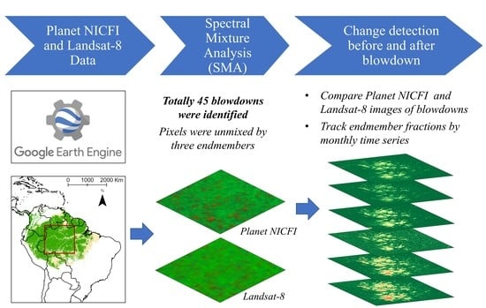
2. Materials and Methods

2.1. Study Sites

Previous studies have shown that blowdowns are most common in the central and northwestern Amazon. For instance, Espírito-Santo et al. [38] found that large blowdown disturbances (>30 ha) are concentrated in the western Brazilian Amazon, with the frequency of large blowdowns being 12 times higher west of 58° W compared to the east [6]. Similarly, Araujo et al. [39] and Negrón-Juárez et al. [40] observed that blowdowns are widespread in the Amazon, ranging from Peru, Colombia, Venezuela, and western Brazil to central Brazil, with the highest incidence in northwestern Amazonia.
In this study, the analyzed blowdown events encompassed a wide range in the Amazon Basin from 15°S–75°W to 2°N–50°W (Figure 1). Although the search was not exhaustive or systematic in nature, we identified 45 blowdowns occurring in Brazil (Amazonas and Mato Grosso states) and Colombia after September 2020. The blowdowns were visually identified in the images from signals of treefalls observed in specific spatial patterns such as the fan-shaped spatial pattern [23]. These spatial patterns were directly associated with changes in NPV and GV fractions caused by blowdowns. Therefore, the occurrence of these spatial patterns separated changes in NPV and GV fractions caused by disturbance from eventual modifications in these fractions derived from vegetation phenology. However, it is important to note that these identified blowdown sites do not represent all blowdown events that occurred during this period but rather a collection used for analysis, which must have occurred after September 2020 in order to have access to the readily available monthly data from PlanetScope NICFI. Thirty-three blowdown events were concentrated in the northern municipality of Barcelos, located in the Brazilian state of Amazonas, northwest of Manaus (0.03°S–61.16°W to 1.22°S–4.81°W). Additionally, five blowdowns were detected in southeast Colombia, along the border with Peru and Brazil (1.35°S–69.96°W to 2.52°S–72.71°W). These areas are predominantly pristine wet rainforest reserves and national parks characterized by a tropical rainforest climate. Furthermore, seven blowdowns occurred in northeast Mato Grosso, Brazil (10.67°S–53.63°W, 11.80°S–53.83°W), which is a transition zone with savanna vegetation. All three regions receive an annual rainfall of over 2000 mm and have less than 4 months with rainfall below 100 mm per year [41].
Figure 1. Study sites with related blowdown events found in the Amazon Forest. The background image corresponds to the areas covered by rainforests and other land covers in the Amazon Forest, according to the Tropical Moist Forests product [42].
Remotesensing 15 03196 g001

2.2. Landsat-8 and PlanetScope NICFI Satellite Data

Surface reflectance data were acquired from the Landsat-8 OLI and PlanetScope NICFI products for the period from September 2020 to May 2022. The atmospherically corrected surface reflectance data from the Landsat-8 OLI sensor are included in Google Earth Engine (GEE)’s USGS Landsat-8 Level 2 Collection, and these images contain four visible, a NIR, and two SWIR bands [43]. Landsat images are selected to form a time series by choosing images where cloud cover does not obscure the blowdown event within each month. In typical cases, Landsat-8 may have several consecutive months where the blowdown event cannot be observed due to cloud cover. In this study, cloud masking using the quality assessment (QA) band was applied to the Landsat-8 images. Similarly, the PlanetScope NICFI monthly mosaics are derived from surface reflectance data from the PlanetScope Dove constellation, having three visible bands and a NIR one [31]. The PlanetScope NICFI data have been subjected to a series of pre-processing, including atmospheric correction, cloud masking, stitching, and seamline removal. Additionally, the PlanetScope NICFI data were already normalized using BRDF-corrected Sentinel-2 data. This strategy reduces the variability added by variable view-illumination conditions, resulting in more reliable and consistent reflectance measurements [37]. Band information and resolution parameters for both datasets are shown in Table 1. Satellite data were acquired using the GEE platform [44].

2.3. Spectral Mixture Analysis (SMA)

SMA estimates the fractional abundance of “pure” spectral components in a pixel [45]. These pure components are called spectral endmembers, for example, non-photosynthetic vegetation (NPV; dry leaves or bare trunk and branches) and green vegetation (GV; photosynthetically active vegetation). Nelson et al. [23] found that the spectral reflectance of recent blowdowns (<1–2 years old) in Landsat imagery showed higher NPV and lower GV fractions compared to the surrounding and pre-blowdown forest. Therefore, the change in NPV (ΔNPV) can be calculated to detect and quantify the intensity of a recent blowdown [26]. In this study, we applied the Linear Spectral Unmixing (LSU) algorithm available on GEE. LSU assumes that the reflectance of a pixel is a linear combination of the endmember spectra (e.g., NPV, GV, and shade). The role of LSU is to unmix their corresponding abundance fractions [46].
Assuming that n is the number of spectral bands for remote-sensing data, we used separately the first seven reflectance bands of Landsat-8 and the four reflectance bands of PlanetScope NICFI as input data to LSU. In this study, NPV, GV, and shade are the endmembers of interest. Additionally, a corresponding vector represents their contributions to the surface reflectance for each pixel, which refers to the cover fractions of endmembers: f = [f1, f2, f3]T. Then, using an n-dimensional vector to represent the pure spectrum of each endmember, the three endmembers are represented as an n × 3 matrix M. Finally, the mixed spectrum of the pixel can be expressed as an n-dimensional vector:
r = M f + ε
where ε is noise or residual error between the model and image reflectance values.
The first step in the SMA procedure is the identification of endmember spectral signature M. M can be obtained from reference spectral libraries derived from field or laboratory measurements [47] but can also be derived directly from the image data [48]. The second step is the estimation of abundance fractions. This requires inversion models to solve for f, and the least squares regression is commonly used to minimize the error term. The output fractions were not constrained to sum to one.
In this study, to avoid differences in data variability caused by instrumental signal-to-noise, we selected the endmembers directly from the images instead of using field or lab reflectance data. This image selection approach has been used in several studies addressing spectral mixture analysis, e.g., [46,49]. Here, we inspected typical areas of endmember occurrence in the images with the support of red–NIR scatterplots. The endmembers were selected on the GEE platform (Figure 2) to represent NPV, GV, and shade endmembers. Endmembers were selected to represent NPV, GV, and shade, and then the training data points were marked for sampling reflectance values (n = 1009 pixels). NPV was collected from the pixels of the fallen crowns and trunk within the blowdown events observed above; GV was sampled from a broad range of green crowns, including secondary forest, recently flushed crowns, and crowns with dark-green mature leaves; shade was collected under clouds. The PlanetScope NICFI product has only four bands in the VNIR interval. Thus, the spectral information is not as complete as that from Landsat-8. There are also differences in the spectral curves of the same endmember between the two datasets (Figure 2). For example, the GV of PlanetScope NICFI has lower reflectance in the green and NIR bands than the reflectance recorded in the corresponding bands of Landsat-8. This is likely because more secondary forests were sampled for the Landsat GV endmembers than for the PlanetScope GV endmembers. We do not expect these differences between sensors to cause significant issues in the analyses, because the focus will not be on the absolute magnitude of fractions but on their change over time.

2.4. Amazon Blowdown Event Mapping and Data Collection

To compare the effects of spatial resolution between PlanetScope NICFI and Landsat-8 on estimating blowdown area, we selected blowdown events with similar acquisition times from both satellite datasets. Specifically, we defined threshold values of ΔNPV (0.3 and 0.5) to quantify the blowdown areas derived from PlanetScope NICFI and Landsat-8 data, and investigated whether there were significant differences between the two datasets. Such ΔNPV thresholds corresponded approximately to minimum and maximum values following disturbance. For GV, the average value pre-disturbance was selected for analysis.
Additionally, because there are few available geolocation data for blowdowns from previous research, a visual interpretation of images was conducted where 45 blowdown events were identified between September 2020 and May 2022. These events showed canopy gap openings varying from less than 1 ha and up to 2026 ha. Landsat-8 and PlanetScope NICFI imagery were interpreted to vectorize the blowdown shapes as polygons in ArcGIS Pro 2.8.3 [50]. For each blowdown, the delineated polygons corresponded to the gaps left by the dead trees in the forest. The geographic reference coordinate system of the polygons was set to WGS84, and each polygon’s area (i.e., geodesic) was then calculated. The first visible month on the image of each blowdown was added as a field of the attribute table. During vectorization, we qualitatively compared the visualization of Landsat-8 and PlanetScope NICFI imaging of blowdown gaps.

2.5. Analysis

Monthly Landsat-8 and PlanetScope NICFI time series were analyzed for each blowdown. This time series started from the three months of available cloud-free images before the blowdown gap was first visible until the gap was not observed at all, or until May 2022. If there were clouds obscuring the blowdown gaps, the image was excluded from the analysis. To observe the vegetation signal recovery process, sample points and polygons were set for the forest gap areas. For samples, the mean NPV, GV, and shade fractions for all Landsat and PlanetScope NICFI time series images were then calculated, along with a 95% confidence interval (CI) around their mean values of three pre-blowdown images. In this way, the chronological changes in the signals and fractions of two satellite data were prepared, and comparisons were performed of the completeness of the change trajectory.
For the image with each blowdown first visible and all images afterwards, the difference in the NPV of the sample pixels between them and the pre-blowdown images (i.e., ΔNPV) was calculated. ΔNPVfirst thus refers to the difference between the average NPV of the first post-blowdown image and of the three pre-blowdown images ( N P V p r e m e a n ). This step allowed us to assess the magnitude of ΔNPV right after the blowdown, that is, the signal closer to the “true maximum change”, and to determine when the blowdown signals reached pre-disturbance levels. The higher the value of ΔNPVfirst, the more severe the damage to the forest [27]. In addition, it is also important to consider that blowdown-affected areas may suffer from delayed tree mortality and browning after the first visible image is acquired, so ΔNPV may increase compared to ΔNPVfirst. To find the maximum ΔNPV, we also search the N P V m a x for each blowdown, which is the maximum NPV value of the blowdown among all months. The difference between N P V m a x and N P V p r e m e a n is the maximum ΔNPV.
We then recorded the ΔNPV change after blowdowns. Instead of recording from the first month the blowdown was found, because the recovery of each blowdown can differ significantly, and starting from the most damaged month (highest ΔNPV) provides a more accurate representation of the recovery process, the average of ΔNPV for all blowdowns and 95% CI were then calculated for each time step, recording the decline process from their maximum value (i.e., 1) to pre-blowdown level.
Similarly, to reflect the process of GV fraction recovery to pre-blowdown levels, the ratio was calculated:
G V i   R a t i o = G V i G V p r e m e a n ,
where G V i is the average GV value of the ith month from also the month when the blowdown had highest NPV (i = 0); G V p r e m e a n is the average GV of the sample pixels of the three pre-blowdown images. The average and its 95% CI of the GV ratio was then calculated for all blowdowns, recording its increase to 1 from the month of the ΔNPV maximum. When this ratio is greater than or equal to 1, the GV fraction has reached or exceeded the average pre-blowdown GV. This calculation is not the same as NPV because a simple ratio can reflect blowdowns’ GV changes.

3. Results

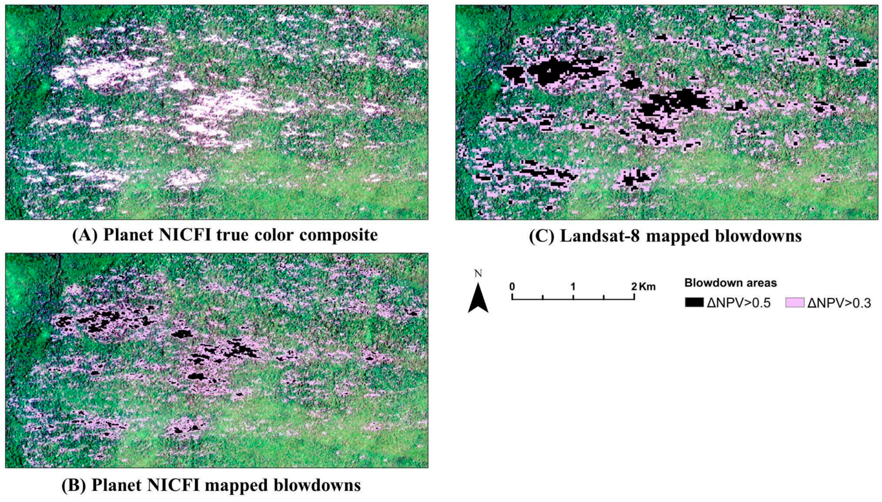
3.1. OLI Landsat-8 and PlanetScope NICFI Images of Blowdown Disturbance

If classified according to the shape of canopy gaps, the blowdowns identified in this study can be divided into three categories: (1) single large gaps (Figure 3(A1,A2)); (2) fan-shaped aggregated gaps (Figure 3(B1,B2)); and (3) discrete clusters of small gaps, whose gaps may not have obvious directional linear characteristics (Figure 3(C1,C2)). Figure 3 also shows the visibility of blowdowns at the different spatial resolutions of Landsat-8 and PlanetScope NICFI images. The single large gaps will usually have a distinct canopy gap which is above 30 ha in size. Fan-shaped aggregated gaps, on the other hand, are fan-shaped aggregations of canopy gaps, which can vary in size from large to small. For discrete clusters of small gaps, they can be seen as a collection of small gaps.
When comparing the ability of Landsat-8 and PlanetScope NICFI satellite datasets to map the area affected by 25 blowdown events using a ΔNPV threshold greater than 0.3 or 0.5 (Table 2), Landsat-8 mapped a larger area (total area = 3809 ha) than PlanetScope NICFI (total area = 3244 ha) when using a threshold of 0.3. However, the use of a higher threshold (ΔNPV > 0.5) reduced the mapped area and led to a similar affected area being mapped by Landsat-8 and PlanetScope NICFI (1962 and 1963 ha, respectively). Furthermore, the number of individual canopy gaps (clusters of pixels mapped as disturbed areas) mapped by PlanetScope NICFI was greater than that of Landsat-8, with 1.4 million pixels of gaps in PlanetScope versus 42 thousand pixels of gaps in Landsat-8. This difference can be observed in Figure 4, where Landsat-8 displays larger contiguous areas of gaps compared to PlanetScope NICFI.

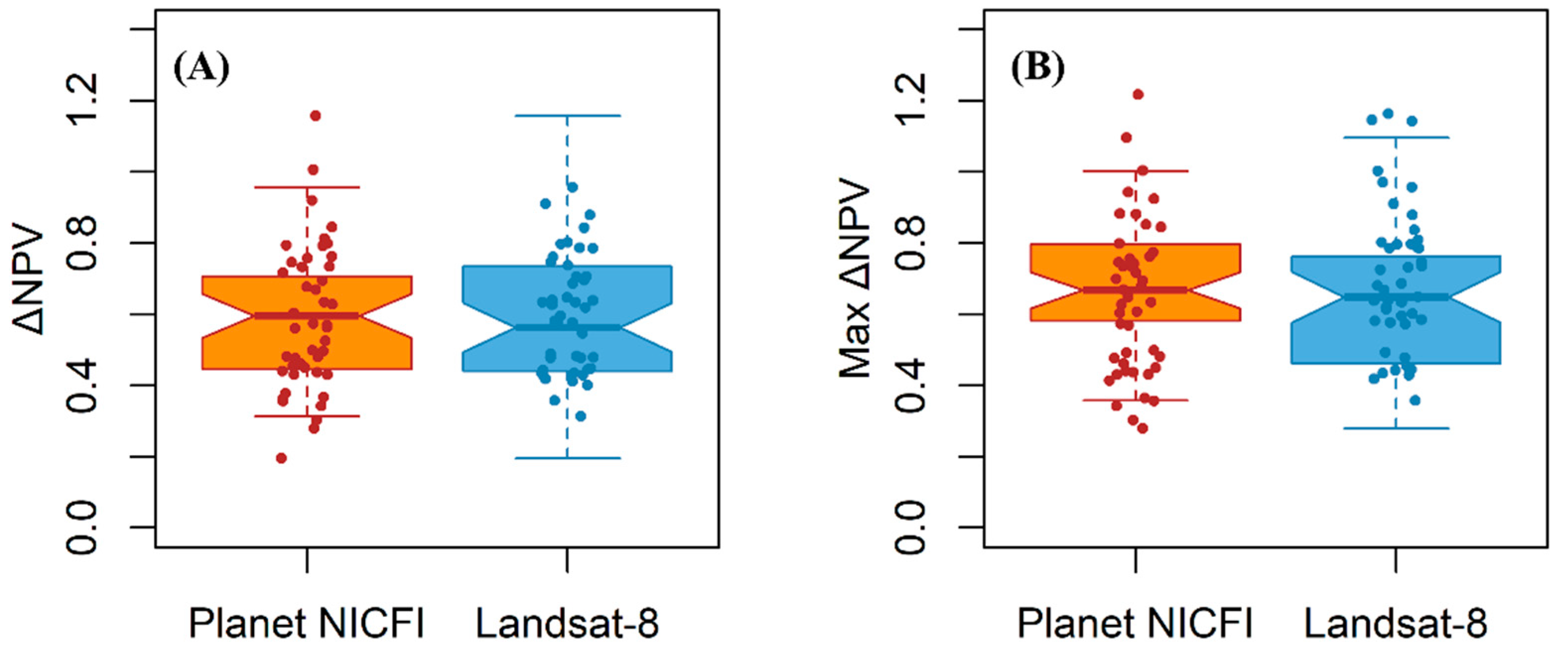
3.2. Changes in Endmember Fractions after Blowdown

The difference (ΔNPVfirst) between the mean NPV in the blowdown first visible image and the mean pre-blowdown raw NPV for both satellites was not significantly different considering a 5% significance level (Figure 5). Most of the ΔNPVfirst values were between 0.3 and 0.8, meaning that the blowdown events generally caused a moderate to substantial decrease in NPV relative to the pre-disturbance conditions, with some sites experiencing more severe damage. However, the fact that the majority of the values fall within this range suggests a relatively consistent impact across the study sites. The maximum ΔNPV for PlanetScope NICFI is larger than its ΔNPVfirst, whereas for Landsat-8, the two attributes are not significantly different. Furthermore, the maximum ΔNPV of PlanetScope NICFI was relatively higher than the distribution of OLI Landsat-8. This indicates that, while the recovery of reflectance values after a disturbance varies between the two satellites, the blowdown events generally caused a moderate to substantial decrease in NPV, with some sites experiencing more severe damage, highlighting the significant impact of these disturbances on the forest ecosystem.

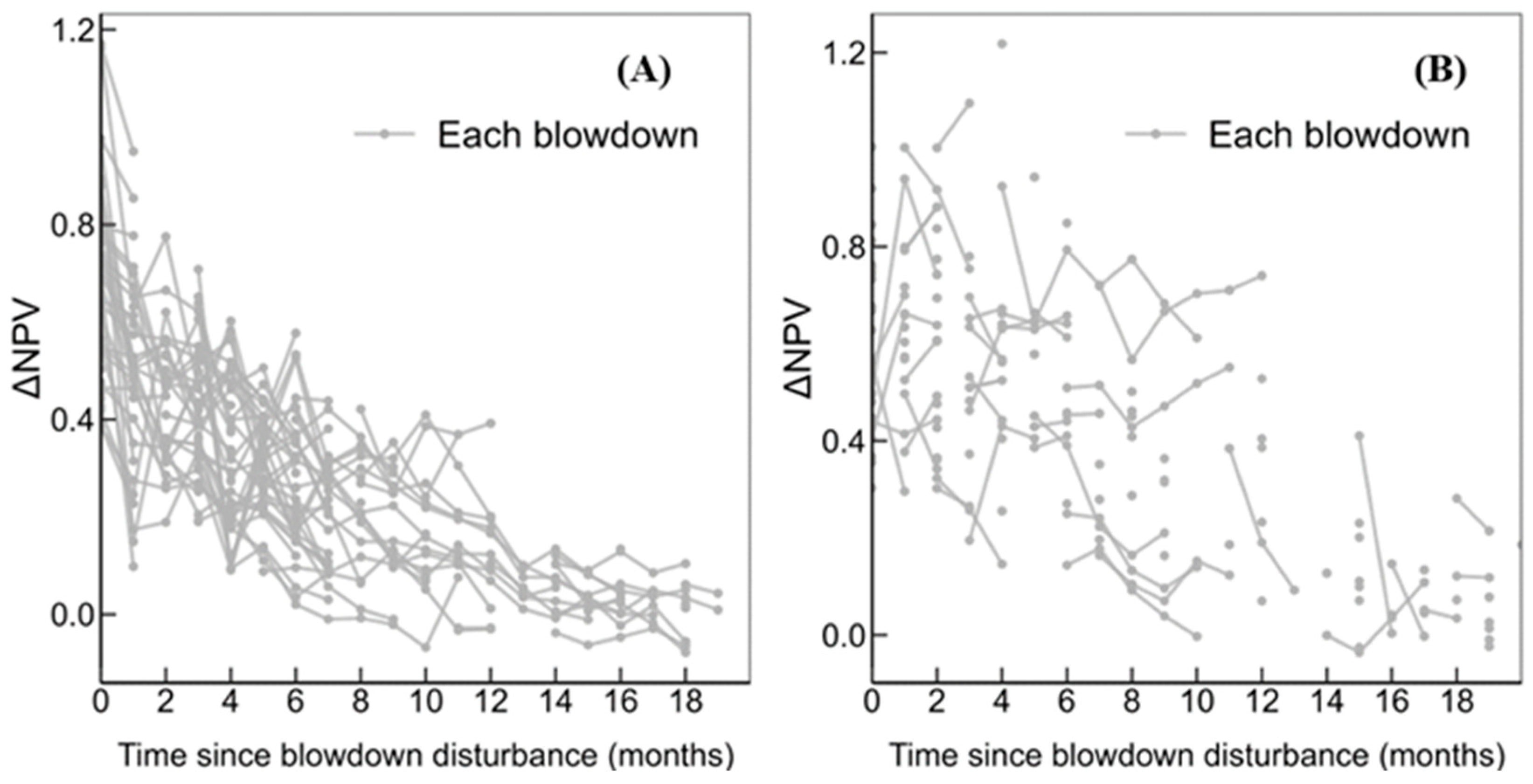
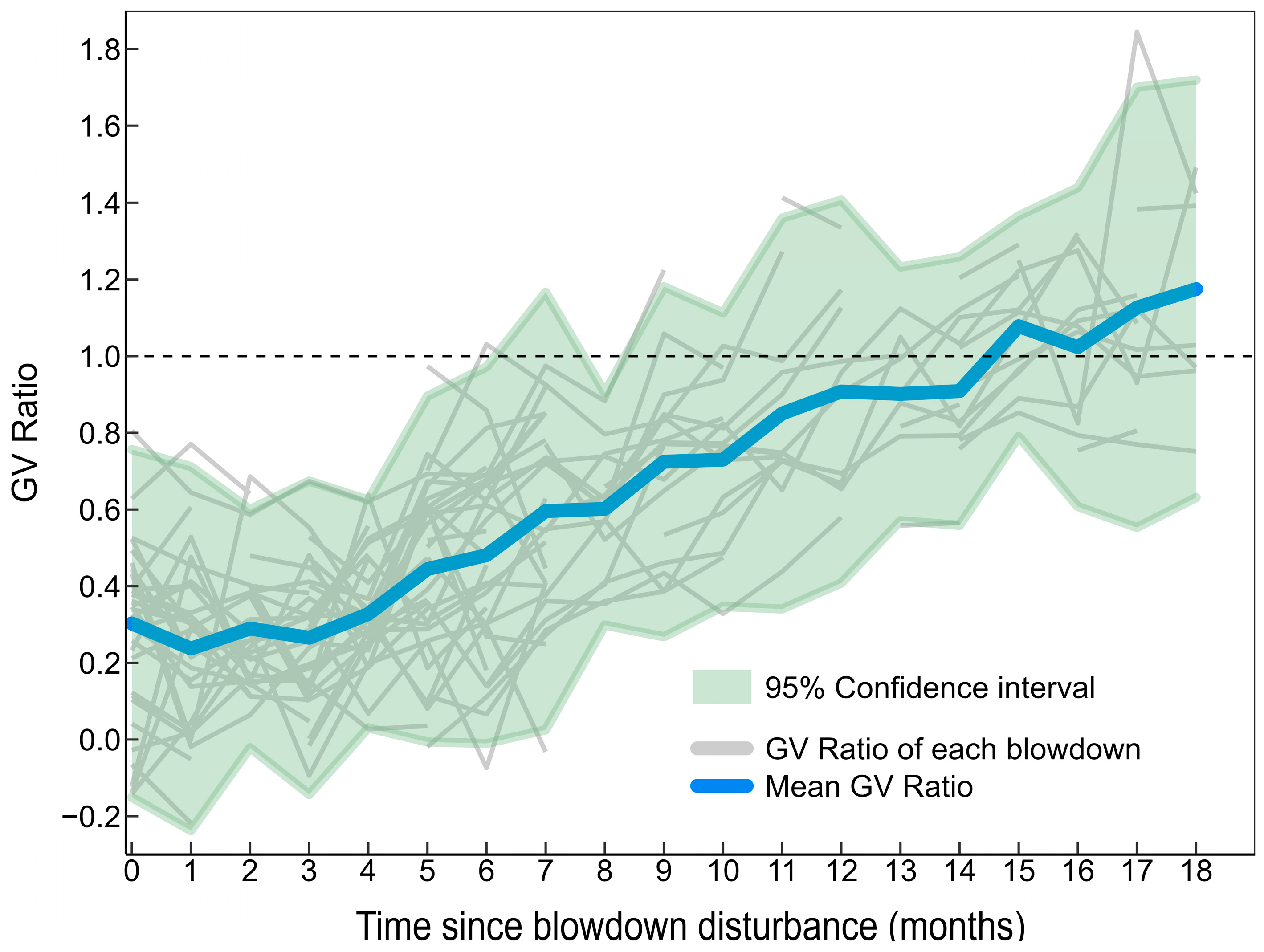
3.3. Post-Blowdown Vegetation Regeneration Process

From the total of 45 analyzed blowdowns, 10 have recovered to a level within the 95% CI of their pre-disturbance NPV mean within 12 months for both Landsat-8 and PlanetScope NICFI data. Whenever the NPV fractions were detected as recovered in the Landsat-8 time series, they were also detected as recovered in PlanetScope NICFI. The opposite was not always the case; 10 blowdowns were identified as recovered in PlanetScope NICFI but not in Landsat-8, likely due to the lack of image acquisitions from Landsat-8. Furthermore, 25 of the 45 blowdowns did not return to pre-disturbance NPV levels after 20 months of observation. For the 20 blowdowns whose time to recover to pre-disturbance levels was detected in PlanetScope NICFI, the shortest recovery was three months and the longest was 20 months, with a mean of 12.2 ± 4.8 months. For the same ten blowdowns in Landsat-8, the average recovery time was similar (14.1 ± 3.1 months) to PlanetScope but with a smaller variance, with a minimum of 8 months and a maximum of 15 months.
Figure 6 shows the trends in ΔNPV for both PlanetScope NICFI and OLI Landsat-8. The start date of each blowdown was determined as the month of the earliest image in which it was detected in either of the two datasets. The trend in NPV fractions in PlanetScope NICFI for all 45 blowdown events is shown in Figure 6A. The trajectory of NPV chronological changes in the PlanetScope NICFI monthly time series was broadly complete and, although fluctuating, showed a generally declining trend. Additionally, many blowdowns did not reach their peak NPV when they were first visible, so NPV did not always fall. This suggests that the extent of damage caused by blowdown events may be underestimated if only the first visible image is used to assess NPV changes. All available Landsat-8 images of blowdowns were included in Figure 6B. Compared to PlanetScope NICFI, the OLI Landsat-8 was not able to provide a consistent ΔNPV trajectory with recovery (Figure 6B) due to difficulties in obtaining regular monthly observations. Although a decrease in ΔNPV over time can be seen, the details of the chronological change are not clear. In the 15 months analyzed after the blowdown, there was an average of 12.9 available cloud-free PlanetScope NICFI images for all blowdown events, compared to only 5.1 images from Landsat-8.
To gain a deeper understanding of the recovery trend of permanent vegetation after blowdown events, we analyzed PlanetScope NICFI images due to limited availability of OLI Landsat-8 images. Upon considering all blowdown events, we observed that the mean ΔNPV curve reached around pre-blowdown level at approximately 15 months or more, and about 17 months to fall completely into the 95% CI of the mean pre-blowdown NPV (Figure 7). This recovery time is longer than the average of 12.3 months and 14.1 months required for the NPV to surpass the lower bound of the 95% confidence interval (CI) around the mean of pre-disturbance NPV. Furthermore, the lower limit of the 95% CI of the mean curve decreased to pre-blowdown level at around 6 months, while the upper limit remained above 0 throughout the study period, which is significantly different from the mean curve, indicating substantial differences in the ΔNPV curves of individual blowdowns.
Although the recovery process varied among the blowdowns, we observed a general trend of ΔNPV decreasing from fast to slow until it reaches around pre-blowdown level. We calculated the average monthly drop starting from the largest observable ΔNPV (Figure 7). It is important to note that the decrease in ΔNPV over time was not linear. The most significant decrease occurred in the first two months, with a drop of 28.05% in the first month and 7.91% in the second month. Additionally, by the fourth month, the average ΔNPV had decreased cumulatively by 52.93%, indicating that the average NPV was less than half of the average maximum NPV during this period.
The ratio of the monthly average GV to pre-blowdown GV also showed that the GV fraction returned to pre-blowdown levels at approximately 15 months, similar to ΔNPV (Figure 8). Overall, it can be considered that these blowdowns recovered to pre-disturbance levels at around 15 months. Similarly, the upper limit of the 95% CI of the average GV ratio curve increased to 1 at about seven months. Moreover, the average GV ratio would continue to grow over time after it reached 1.
Figure 9 depicts the complete course of one blowdown from pre-blowdown to its NPV return to the 95% CI of pre-blowdown mean NPV by 17 months of regeneration. The blowdown reached its maximum NPV in the second month of visibility (October 2020), after which it began to decline gradually. The NPV seems to decrease more quickly for the smaller gaps, whereas the larger gaps decrease more slowly. In the last image of the panel (February 2022), the southern part of the blowdown is no longer visible in the PlanetScope NICFI optical imagery.

4. Discussion

The current study employed both PlanetScope NICFI and Landsat-8 data to analyze the trajectory of spectral recovery in vegetation after blowdown events. Our findings indicate that determining the date of blowdown disturbance plays a key role when estimating damage using traditional remote-sensing-based methodologies based on the ΔNPV. PlanetScope NICFI data provide a more effective monitoring capability compared to Landsat data due to its enhanced temporal resolution, which allows it to identify the precise date of blowdown occurrence. Furthermore, our findings also show that the apparent effects of blowdown on vegetation as observed by the satellite imagery may fade away after 15 months of recovery. Therefore, blowdown detection at annual intervals would likely be required in order not to miss disturbance events, which could be achieved either using Landsat or PlanetScope NICFI datasets. Then, determining the date of disturbance can come on a later stage using a denser time series of PlanetScope, Sentinel-2 or Landsat satellites to achieve a more exact date of disturbance. Moreover, our results highlight the importance of considering a regular monthly time scale as a minimum requisite for estimating the date of which blowdown events occurred. Using this approach, we can more accurately estimate damage caused by blowdowns. In contrast, missing this time window may result in underestimating the disturbance by a significant percentage. For instance, ΔNPV decreased in 28.47% in the first month post-disturbance, and up to 50% by four months post-disturbance. Therefore, if the change in ΔNPV is used as a way to estimate wind damage, time since disturbance becomes a crucial factor that must be considered in the analysis. This study is the first to address the spectral trajectory of blowdown events on a regular monthly basis using the PlanetScope NICFI program. Our results demonstrate its strong potential for accurate estimation of vegetation damage and subsequent recovery. Further use of daily observations can refine this knowledge.
Our findings show that identifying the precise date of blowdown occurrence can have significant impact for consistent damage estimation using the ΔNPV approach. When detecting the disturbance of blowdown with the variation in non-photosynthetic vegetation (ΔNPV), a simple threshold method is usually used in the literature [25,51,52], that is, when the ΔNPV of a pixel is greater than a critical value, it is considered to be turned into a blowdown gap. For instance, Negrón-Juárez et al. [25] consider 0.06 and Marra et al. [51] set it to 0.16. According to our results, this critical value depends on how many months of recovery have gone by when the imagery is obtained. Therefore, in order to apply the ΔNPV method over larger areas, one would need to know the exact date of blowdown occurrence, or one would incur an underestimation of the actual tree mortality. For example, a linear regression between field and remote-sensing data for imagery acquired six months after blowdown [27] will have much lower NPV values than if the imagery was acquired right after disturbance. The use of such an equation would have to be cautious to consider at the same time since disturbance. Therefore, we strongly suggest that integrating field data with remote-sensing estimates must take into account time since disturbance; otherwise, the established relationships will not be reliable for extrapolation in other areas. While we have only investigated spectral mixture fractions—the most traditional data used for blowdown damage estimates—the presented results can likely be generalized to other vegetation indices, as the spectral recovery with vegetation recovery is also reflected on other spectral bands and vegetation indices [53].
PlanetScope NICFI data provided a more reliable identification of the maximum ΔNPV after blowdown occurrence than Landsat-8. The reason is that the continuous cloudless images make PlanetScope NICFI data easier to identify the true maximum change. For instance, we had an average of 12.9 PlanetScope NICFI images available in 15 months of analysis. In contrast, Landsat-8 had a much lower number of cloud-free images (average 5.1 in 15 months). The first available post-blowdown image of Landsat-8 was found on average after ~1.1 months; therefore, recovery is already in place and the maximum change can be lost. As we already presented, our analyses show that ΔNPV decreases by 28.47% in the first month post-disturbance. For example, in a study of tree mortality in the Amazon Forest following a squall line event in 2005 [27], the first image captured after the blowdown occurred 6 months later, potentially underestimating tree mortality due to rapid growth of pioneer species that covered the dead trunks and branches, decreasing the NPV fraction [25,27,51]. According to our analyses, after six post-disturbance months, the ΔNPV signal may have recovered an average of around 60%. Therefore, while models relating ΔNPV to tree loss may work well if calibrated locally for specific sets of images, they would not be easily applied to other areas if imagery is collected with a different time since disturbance.
Additionally, the spatial resolution of the satellite sensor used for mapping blowdowns can affect the accuracy of the estimates. In particular, we observed that Landsat-8 OLI tends to overestimate the area of disturbance, especially when using a lower threshold (ΔNPV > 0.3) to capture more subtle changes. This overestimation may be due to the coarser resolution of Landsat-8 data compared to PlanetScope NICFI. However, when a more conservative or higher threshold (ΔNPV > 0.5) was used, therefore mapping only the more severely damaged areas, the area mapped by Landsat-8 and PlanetScope NICFI was similar. It is important to consider these differences in mapping blowdowns for accurate estimation of the extent of disturbance and its impact on ecosystem dynamics. Further research is needed to investigate the effect of spatial resolution on other ecosystem disturbances and to determine the appropriate threshold values for different satellite sensors.
Similarly, the use of high-spatial-and-temporal-resolution data is important for further estimating the loss of biomass and carbon in forest ecosystems caused by wind disturbances. Previous studies have focused on the loss of carbon and biomass caused by blowdowns [6,25,54]. However, using open optical imaging data such as Landsat-8 and Sentinel-2 to identify forest disturbances may inaccurately estimate tree mortality rates and the loss of biomass and carbon. In contrast, higher-spatial-and-temporal-resolution data can detect smaller blowdowns and potentially obtain more usable images closer to the most severe disturbance, enabling more accurate estimation of these damages. Against the backdrop of global warming, windthrow density in the Amazon region may further increase [2], which could result in more blowdown events in the future. With the goal of carbon neutrality in mind, the increase in blowdowns will undoubtedly increase the pressure on carbon sequestration in the Amazon Forest. Accurately measuring the loss of biomass and carbon after blowdowns in the future could be helpful for forest conservation policies and carbon offset programs.
For all the 45 blowdowns, we show that the spectral response of vegetation recovers on average after about 15 months since disturbance (Figure 7 and Figure 8). It is expected that the small gaps recover faster than the large ones, which, although not explicitly quantified, can be seen in the example of Figure 9. This is in line with previous studies estimating recovery time to be around one year [25,27,29]. However, it is important to note that even though the ΔNPV reaches pre-blowdown levels, it does not necessarily indicate full recovery of vegetation but merely that the spectral properties of the vegetation resemble those of pre-disturbance. The gap contours and shape of blowdowns (Figure 9) are still visible after recovery, suggesting that the pioneer vegetation within the gap is still in the growing stage and has not yet fully reached the level of the surrounding mature forest. Thus, longer observation periods are needed to determine if the regenerated vegetation will eventually reach maturity. The previous literature on gap recovery in tropical forests also shows that small gaps fully close in less than two years and larger gaps may take longer and up to five years to close while some may still be visible [15]. This could be due to the larger area occupied by fallen tree bases in bigger gaps, which can hinder the growth and regeneration of seedlings [55]. Therefore, we suggest future studies to stratify analysis of blowdown recovery time by gap size to further quantify these effects.
Comparing Figure 6A,B, PlanetScope NICFI is more appropriate for monitoring the post-blowdown vegetation recovery process because it produces more coherent curves than Landsat-8. In terms of forest regeneration models, blowdowns are one of the gap disturbances, while the land cover type does not change, and the forest will gradually regenerate [56,57]. Furthermore, Figure 6A also shows that post-blowdown forest regeneration is a complex process. NPV fraction sometimes fluctuates upwards during the gradual decline following blowdown disturbance. This phenomenon could be attributed to delayed tree mortality following the disturbance, as noted by Henkel et al. [58]. Possible contributing factors to this phenomenon include further damage to native and emergent vegetation by additional strong winds during the revegetation period or increased mortality of old trees within the sample pixels due to the gap created by the blowdown, which exposes them to disturbance, changes in microclimate, or other unknown reasons. In conclusion, not all trees perish during blowdown disturbances, and determining the exact cause of tree mortality post-blowdown remains a complex and unresolved issue [28].
However, it is important to highlight here that the vegetation recovery tracking in this study only included the blowdowns in the early growth stages of pioneer species. It did not follow blowdowns for longer than two years. This is because the NICFI program is only open for monthly mosaics whose date is after September 2020, before which only 3-month or 6-month mosaics are open. To obtain consistent monthly images, only blowdown events occurring after September 2020 and no later than May 2022 have been selected for this study. The PlanetScope NICFI catalog can be used in further studies which encompass mosaics produced monthly up to this day and expected until August 2024. While we have only investigated spectral mixture fractions—the most traditional data used for blowdown damage estimates—the presented results can likely be generalized to other vegetation indices, as the spectral recovery with vegetation recovery is also reflected on other spectral bands and vegetation indices [53].
One of the main contributions of this study is the understanding of ΔNPV variability over time with recovery after blowdown occurrences. The studies on the detection of post-blowdown forest regeneration are limited to several discrete time points (e.g., six months, two years) after the blowdowns, but now, we raise the point that if we want to make consistent tree mortality estimates due to wind disturbances, a time series of observations would be required to correct for time since disturbance. One of the next steps in this research subject is to model ΔNPV over time for blowdowns that consider multiple influencing factors. The observed relationships between time since disturbance and ΔNPV may be used to calibrate models that assess forest damage due to blowdowns. Since the window for detecting blowdowns is short, if this period is missed, then the approximate loss can also be predicted from the model. Another point is to consider differential recovery rates in tropical forests, which was not explored in this study due to the limited database of blowdowns. A more comprehensive database of blowdowns needs to be gathered in order to analyze effects of recovery due to environmental and climate gradients [59,60]. Furthermore, SAR data have not traditionally been used for blowdown analyses in the Amazon, but due to the relationship between SAR and vegetation structure [61], it could potentially be used to analyze the blowdown trajectories over time and determine the exact date of disturbance. SAR data in general are less affected by weather conditions than optical data [62], and this factor should contribute to obtaining a reliable time series for the accurate retrieval of the date of blowdown disturbance.

5. Conclusions

We investigated the patterns of blowdowns in tropical forests, including their potential mapping using Landsat-8 and PlanetScope satellite optical sensors, estimating their damage and tracking post-disturbance forest regeneration and dynamics. We concluded that the higher temporal and spatial resolution of PlanetScope NICFI imagery, compared to Landsat-8 OLI, allowed for monitoring the effects of blowdown disturbances and vegetation recovery much more consistently. We highlighted the importance of detecting the precise date of disturbance in order to consistently estimate tree mortality associated with blowdowns. The regular monthly time scale of the NICFI product used here can be considered as a minimum requisite for estimating the date of occurrence of the blowdown events. This information can be further refined with daily observations of other products. The consistent estimation of tree mortality associated with blowdown occurrence in future studies should require the detection of blowdown occurrence. Otherwise, damage may be significantly underestimated, for instance, in 52.93% in only four months of delay from disturbance to the first acquired image. Moreover, our study revealed that the NPV fraction obtained from the PlanetScope NICFI monthly mosaics recovered to pre-disturbance levels (95% confidence interval) after an average of 12.2 months since disturbance. We note the recovery may vary with differences in gap size. Thus, the stratification of blowdowns by gap size is a future research direction that deserves further investigation.

Author Contributions

Conceptualization, D.P., R.D. and P.d.C.B.; methodology, D.P., R.D. and P.d.C.B.; software, D.P.; validation, D.P.; formal analysis, D.P. and R.D.; investigation, D.P. and R.D.; resources, D.P., R.D. and P.d.C.B.; data curation, D.P.; writing—original draft preparation, D.P.; writing—review and editing, R.D., L.S.G., B.N., F.W., D.M.S. and P.d.C.B.; visualization, D.P.; supervision, R.D. and P.d.C.B. All authors have read and agreed to the published version of the manuscript.

Funding

This research received no external funding.

Data Availability Statement

The shapefile of polygons of blowdown events in this study are available at: https://zenodo.org/record/7036241 (accessed on 20 April 2023).

Acknowledgments

The authors thank the Department of Geography, School of Environment Education and Development (SEED) at the University of Manchester (UK) for the support on this research.

Conflicts of Interest

The authors declare no conflict of interest.

References

  1. Negrón-Juárez, R.I.; Jenkins, H.S.; Raupp, C.F.; Riley, W.J.; Kueppers, L.M.; Magnabosco Marra, D.; Ribeiro, G.H.; Monteiro, M.T.F.; Candido, L.A.; Chambers, J.Q. Windthrow Variability in Central Amazonia. Atmosphere 2017, 8, 28. [Google Scholar] [CrossRef] [Green Version]
  2. Feng, Y.; Negrón-Juárez, R.I.; Romps, D.M.; Chambers, J.Q. Amazon Windthrow Disturbances Are Likely to Increase with Storm Frequency under Global Warming. Nat. Commun. 2023, 14, 101. [Google Scholar] [CrossRef] [PubMed]
  3. Tyukavina, A.; Hansen, M.C.; Potapov, P.V.; Stehman, S.V.; Smith-Rodriguez, K.; Okpa, C.; Aguilar, R. Types and Rates of Forest Disturbance in Brazilian Legal Amazon, 2000–2013. Sci. Adv. 2017, 3, e1601047. [Google Scholar] [CrossRef] [PubMed] [Green Version]
  4. Gora, E.M.; Bitzer, P.M.; Burchfield, J.C.; Gutierrez, C.; Yanoviak, S.P. The Contributions of Lightning to Biomass Turnover, Gap Formation and Plant Mortality in a Tropical Forest; John Wiley & Sons: Hoboken, NJ, USA, 2021; ISBN 0012-9658. [Google Scholar]
  5. Chambers, J.Q.; Negron-Juarez, R.I.; Marra, D.M.; Di Vittorio, A.; Tews, J.; Roberts, D.; Ribeiro, G.H.; Trumbore, S.E.; Higuchi, N. The Steady-State Mosaic of Disturbance and Succession across an Old-Growth Central Amazon Forest Landscape. Proc. Natl. Acad. Sci. USA 2013, 110, 3949–3954. [Google Scholar] [CrossRef] [PubMed] [Green Version]
  6. Espírito-Santo, F.D.; Gloor, M.; Keller, M.; Malhi, Y.; Saatchi, S.; Nelson, B.; Junior, R.C.O.; Pereira, C.; Lloyd, J.; Frolking, S. Size and Frequency of Natural Forest Disturbances and the Amazon Forest Carbon Balance. Nat. Commun. 2014, 5, 1–6. [Google Scholar] [CrossRef] [Green Version]
  7. Peterson, C.J.; Ribeiro, G.H.P.d.M.; Negrón-Juárez, R.; Marra, D.M.; Chambers, J.Q.; Higuchi, N.; Lima, A.; Cannon, J.B. Critical Wind Speeds Suggest Wind Could Be an Important Disturbance Agent in Amazonian Forests. For. Int. J. For. Res. 2019, 92, 444–459. [Google Scholar] [CrossRef]
  8. Esquivel-Muelbert, A.; Phillips, O.L.; Brienen, R.J.; Fauset, S.; Sullivan, M.J.; Baker, T.R.; Chao, K.-J.; Feldpausch, T.R.; Gloor, E.; Higuchi, N. Tree Mode of Death and Mortality Risk Factors across Amazon Forests. Nat. Commun. 2020, 11, 5515. [Google Scholar] [CrossRef] [PubMed]
  9. Lindenmayer, D.; McCarthy, M.A. Congruence between Natural and Human Forest Disturbance: A Case Study from Australian Montane Ash Forests. For. Ecol. Manag. 2002, 155, 319–335. [Google Scholar] [CrossRef]
  10. Kimmins, J.P. Forest Ecology. In Fishes and Forestry: Worldwide Watershed Interactions and Management; Wiley-Blackwell: Hoboken, NJ, USA, 2004; pp. 17–43. [Google Scholar]
  11. Feng, Y.; Negrón-Juárez, R.I.; Chambers, J.Q. Remote Sensing and Statistical Analysis of the Effects of Hurricane María on the Forests of Puerto Rico. Remote Sens. Environ. 2020, 247, 111940. [Google Scholar] [CrossRef]
  12. Urquiza Muñoz, J.D.; Magnabosco Marra, D.; Negrón-Juarez, R.I.; Tello-Espinoza, R.; Alegría-Muñoz, W.; Pacheco-Gómez, T.; Rifai, S.W.; Chambers, J.Q.; Jenkins, H.S.; Brenning, A. Recovery of Forest Structure Following Large-Scale Windthrows in the Northwestern Amazon. Forests 2021, 12, 667. [Google Scholar] [CrossRef]
  13. Gorgens, E.B.; Keller, M.; Jackwon, T.D.; Marra, D.M.; Reis, C.R.; Almeida, D.R.A.; Coomes, D.; Ometto, J.P. Tracking Canopy Gap Dynamics across Four Sites in the Brazilian Amazon. bioRxiv, 2022; preprint. [Google Scholar] [CrossRef]
  14. Chambers, J.Q.; Asner, G.P.; Morton, D.C.; Anderson, L.O.; Saatchi, S.S.; Espírito-Santo, F.D.; Palace, M.; Souza, C., Jr. Regional Ecosystem Structure and Function: Ecological Insights from Remote Sensing of Tropical Forests. Trends Ecol. Evol. 2007, 22, 414–423. [Google Scholar] [CrossRef] [PubMed]
  15. Dalagnol, R.; Phillips, O.L.; Gloor, E.; Galvão, L.S.; Wagner, F.H.; Locks, C.J.; Aragão, L.E. Quantifying Canopy Tree Loss and Gap Recovery in Tropical Forests under Low-Intensity Logging Using VHR Satellite Imagery and Airborne LiDAR. Remote Sens. 2019, 11, 817. [Google Scholar] [CrossRef] [Green Version]
  16. Dalagnol, R.; Wagner, F.H.; Galvão, L.S.; Streher, A.S.; Phillips, O.L.; Gloor, E.; Pugh, T.A.; Ometto, J.P.; Aragão, L.E. Large-Scale Variations in the Dynamics of Amazon Forest Canopy Gaps from Airborne Lidar Data and Opportunities for Tree Mortality Estimates. Sci. Rep. 2021, 11, 1388. [Google Scholar] [CrossRef] [PubMed]
  17. Reis, C.R.; Jackson, T.D.; Gorgens, E.B.; Dalagnol, R.; Jucker, T.; Nunes, M.H.; Ometto, J.P.; Aragão, L.E.; Rodriguez, L.C.E.; Coomes, D.A. Forest Disturbance and Growth Processes Are Reflected in the Geographical Distribution of Large Canopy Gaps across the Brazilian Amazon. J. Ecol. 2022, 110, 2971–2983. [Google Scholar] [CrossRef]
  18. Jucker, T. Deciphering the Fingerprint of Disturbance on the Three-dimensional Structure of the World’s Forests. N. Phytol. 2022, 233, 612–617. [Google Scholar] [CrossRef] [PubMed]
  19. Simonetti, A.; Araujo, R.F.; Celes, C.H.S.; da Silva e Silva, F.R.; dos Santos, J.; Higuchi, N.; Trumbore, S.; Marra, D.M. Gap Geometry, Seasonality and Associated Losses of Biomass–Combining UAV Imagery and Field Data from a Central Amazon Forest. Biogeosciences Discuss. 2023. [Google Scholar] [CrossRef]
  20. McConnell, T.J. A Guide to Conducting Aerial Sketchmapping Surveys; US Department of Agriculture, Forest Service: Washington, DC, USA, 2000.
  21. Stone, C.; Carnegie, A.; Melville, G.; Smith, D.; Nagel, M. Aerial Mapping Canopy Damage by the Aphid Essigella Californica in a Pinus Radiata Plantation in Southern New South Wales: What Are the Challenges? Aust. For. 2013, 76, 101–109. [Google Scholar] [CrossRef]
  22. Stone, C.; Mohammed, C. Application of Remote Sensing Technologies for Assessing Planted Forests Damaged by Insect Pests and Fungal Pathogens: A Review. Curr. For. Rep. 2017, 3, 75–92. [Google Scholar] [CrossRef]
  23. Nelson, B.W.; Kapos, V.; Adams, J.B.; Oliveira, W.J.; Braun, O.P. Forest Disturbance by Large Blowdowns in the Brazilian Amazon. Ecology 1994, 75, 853–858. [Google Scholar] [CrossRef]
  24. Chambers, J.Q.; Negrón-Juárez, R.I.; Hurtt, G.C.; Marra, D.M.; Higuchi, N. Lack of Intermediate-scale Disturbance Data Prevents Robust Extrapolation of Plot-level Tree Mortality Rates for Old-growth Tropical Forests. Ecol. Lett. 2009, 12, E22–E25. [Google Scholar] [CrossRef]
  25. Negrón-Juárez, R.I.; Chambers, J.Q.; Marra, D.M.; Ribeiro, G.H.; Rifai, S.W.; Higuchi, N.; Roberts, D. Detection of Subpixel Treefall Gaps with Landsat Imagery in Central Amazon Forests. Remote Sens. Environ. 2011, 115, 3322–3328. [Google Scholar] [CrossRef]
  26. Chambers, J.Q.; Fisher, J.I.; Zeng, H.; Chapman, E.L.; Baker, D.B.; Hurtt, G.C. Hurricane Katrina’s Carbon Footprint on US Gulf Coast Forests. Science 2007, 318, 1107. [Google Scholar] [CrossRef] [PubMed] [Green Version]
  27. Negrón-Juárez, R.I.; Chambers, J.Q.; Guimaraes, G.; Zeng, H.; Raupp, C.F.; Marra, D.M.; Ribeiro, G.H.; Saatchi, S.S.; Nelson, B.W.; Higuchi, N. Widespread Amazon Forest Tree Mortality from a Single Cross-basin Squall Line Event. Geophys. Res. Lett. 2010, 37, L16701. [Google Scholar] [CrossRef]
  28. Rifai, S.W.; Urquiza Muñoz, J.D.; Negrón-Juárez, R.I.; Ramírez Arévalo, F.R.; Tello-Espinoza, R.; Vanderwel, M.C.; Lichstein, J.W.; Chambers, J.Q.; Bohlman, S.A. Landscape-scale Consequences of Differential Tree Mortality from Catastrophic Wind Disturbance in the Amazon. Ecol. Appl. 2016, 26, 2225–2237. [Google Scholar] [CrossRef] [Green Version]
  29. Chambers, J.Q.; Robertson, A.L.; Carneiro, V.M.; Lima, A.J.; Smith, M.-L.; Plourde, L.C.; Higuchi, N. Hyperspectral Remote Detection of Niche Partitioning among Canopy Trees Driven by Blowdown Gap Disturbances in the Central Amazon. Oecologia 2009, 160, 107–117. [Google Scholar] [CrossRef] [PubMed]
  30. Weishampel, J.F.; Drake, J.B.; Cooper, A.; Blair, J.B.; Hofton, M. Forest Canopy Recovery from the 1938 Hurricane and Subsequent Salvage Damage Measured with Airborne LiDAR. Remote Sens. Environ. 2007, 109, 142–153. [Google Scholar] [CrossRef]
  31. Wulder, M.A.; White, J.C.; Gillis, M.D.; Walsworth, N.; Hansen, M.C.; Potapov, P. Multiscale Satellite and Spatial Information and Analysis Framework in Support of a Large-Area Forest Monitoring and Inventory Update. Environ. Monit. Assess 2010, 170, 417–433. [Google Scholar] [CrossRef] [Green Version]
  32. Cushman, K.C.; Burley, J.T.; Imbach, B.; Saatchi, S.S.; Silva, C.E.; Vargas, O.; Zgraggen, C.; Kellner, J.R. Impact of a Tropical Forest Blowdown on Aboveground Carbon Balance. Sci. Rep. 2021, 11, 11279. [Google Scholar] [CrossRef]
  33. Emmert, L.; Negrón-Juárez, R.I.; Chambers, J.Q.; Santos, J.D.; Lima, A.J.N.; Trumbore, S.; Marra, D.M. Sensitivity of Optical Satellites to Estimate Windthrow Tree-Mortality in a Central Amazon Forest. Preprints 2023, 2023051631. [Google Scholar] [CrossRef]
  34. Schwarz, M.; Steinmeier, C.; Holecz, F.; Stebler, O.; Wagner, H. Detection of Windthrow in Mountainous Regions with Different Remote Sensing Data and Classification Methods. Scand. J. For. Res. 2003, 18, 525–536. [Google Scholar] [CrossRef]
  35. Negrón-Juárez, R.I.; Holm, J.A.; Faybishenko, B.; Magnabosco-Marra, D.; Fisher, R.A.; Shuman, J.K.; de Araujo, A.C.; Riley, W.J.; Chambers, J.Q. Landsat Near-Infrared (NIR) Band and ELM-FATES Sensitivity to Forest Disturbances and Regrowth in the Central Amazon. Biogeosciences 2020, 17, 6185–6205. [Google Scholar] [CrossRef]
  36. NICFI Securing Tropical Forests for the Future. 2023. Available online: https://www.nicfi.no/ (accessed on 19 April 2023).
  37. Planet NICFI DATA Program User Guide. 2022. Available online: https://assets.planet.com/docs/NICFI_UserGuidesFAQ.pdf (accessed on 29 August 2022).
  38. Espírito-Santo, F.D.; Keller, M.; Braswell, B.; Nelson, B.W.; Frolking, S.; Vicente, G. Storm Intensity and Old-growth Forest Disturbances in the Amazon Region. Geophys. Res. Lett. 2010, 37, L11403. [Google Scholar] [CrossRef] [Green Version]
  39. Araujo, R.F.; Nelson, B.W.; Celes, C.H.S.; Chambers, J.Q. Regional Distribution of Large Blowdown Patches across Amazonia in 2005 Caused by a Single Convective Squall Line. Geophys. Res. Lett. 2017, 44, 7793–7798. [Google Scholar] [CrossRef] [Green Version]
  40. Negrón-Juárez, R.I.; Holm, J.A.; Marra, D.M.; Rifai, S.W.; Riley, W.J.; Chambers, J.Q.; Koven, C.D.; Knox, R.G.; McGroddy, M.E.; Di Vittorio, A.V. Vulnerability of Amazon Forests to Storm-Driven Tree Mortality. Environ. Res. Lett. 2018, 13, 054021. [Google Scholar] [CrossRef]
  41. de Assis Diniz, F.; Ramos, A.M.; Rebello, E.R.G. Brazilian Climate Normals for 1981–2010. Pesqui. Agropecuária Bras. 2018, 53, 131–143. [Google Scholar] [CrossRef]
  42. Vancutsem, C.; Achard, F.; Pekel, J.-F.; Vieilledent, G.; Carboni, S.; Simonetti, D.; Gallego, J.; Aragao, L.E.; Nasi, R. Long-Term (1990–2019) Monitoring of Forest Cover Changes in the Humid Tropics. Sci. Adv. 2021, 7, eabe1603. [Google Scholar] [CrossRef]
  43. USGS Landsat Collection 2 Surface Reflectance. 2022. Available online: https://www.usgs.gov/landsat-missions/landsat-collection-2-surface-reflectance (accessed on 18 August 2022).
  44. Gorelick, N.; Hancher, M.; Dixon, M.; Ilyushchenko, S.; Thau, D.; Moore, R. Google Earth Engine: Planetary-Scale Geospatial Analysis for Everyone. Remote Sens. Environ. 2017, 202, 18–27. [Google Scholar] [CrossRef]
  45. Roberts, D.A.; Smith, M.O.; Adams, J.B. Green Vegetation, Nonphotosynthetic Vegetation, and Soils in AVIRIS Data. Remote Sens. Environ. 1993, 44, 255–269. [Google Scholar] [CrossRef]
  46. Bangira, T.; Alfieri, S.M.; Menenti, M.; Van Niekerk, A.; Vekerdy, Z. A Spectral Unmixing Method with Ensemble Estimation of Endmembers: Application to Flood Mapping in the Caprivi Floodplain. Remote Sens. 2017, 9, 1013. [Google Scholar] [CrossRef] [Green Version]
  47. Roberts, D.A.; Gardner, M.; Church, R.; Ustin, S.; Scheer, G.; Green, R.O. Mapping Chaparral in the Santa Monica Mountains Using Multiple Endmember Spectral Mixture Models. Remote Sens. Environ. 1998, 65, 267–279. [Google Scholar]
  48. Combe, J.-P.; Le Mouélic, S.; Sotin, C.; Gendrin, A.; Mustard, J.F.; Le Deit, L.; Launeau, P.; Bibring, J.-P.; Gondet, B.; Langevin, Y. Analysis of OMEGA/Mars Express Data Hyperspectral Data Using a Multiple-Endmember Linear Spectral Unmixing Model (MELSUM): Methodology and First Results. Planet. Space Sci. 2008, 56, 951–975. [Google Scholar] [CrossRef]
  49. Yang, J.; Weisberg, P.J.; Bristow, N.A. Landsat Remote Sensing Approaches for Monitoring Long-Term Tree Cover Dynamics in Semi-Arid Woodlands: Comparison of Vegetation Indices and Spectral Mixture Analysis. Remote Sens. Environ. 2012, 119, 62–71. [Google Scholar] [CrossRef]
  50. ESRI, A.P. 2.8. 3; Environmental Systems Research Institute. 2021. Available online: https://www.esri.com/content/dam/esrisites/en-us/media/legal/vpats/arcgis-pro-28-vpat.pdf (accessed on 20 April 2023).
  51. Marra, D.M.; Chambers, J.Q.; Higuchi, N.; Trumbore, S.E.; Ribeiro, G.H.; Dos Santos, J.; Negrón-Juárez, R.I.; Reu, B.; Wirth, C. Large-Scale Wind Disturbances Promote Tree Diversity in a Central Amazon Forest. PLoS ONE 2014, 9, e103711. [Google Scholar] [CrossRef] [PubMed]
  52. Di Vittorio, A.V.; Negrón-Juárez, R.I.; Higuchi, N.; Chambers, J.Q. Tropical Forest Carbon Balance: Effects of Field-and Satellite-Based Mortality Regimes on the Dynamics and the Spatial Structure of Central Amazon Forest Biomass. Environ. Res. Lett. 2014, 9, 034010. [Google Scholar] [CrossRef] [Green Version]
  53. Galvão, L.S.; dos Santos, J.R.; da Silva, R.D.; da Silva, C.V.; Moura, Y.M.; Breunig, F.M. Following a Site-Specific Secondary Succession in the Amazon Using the Landsat CDR Product and Field Inventory Data. Int. J. Remote Sens. 2015, 36, 574–596. [Google Scholar] [CrossRef]
  54. Wohl, E. Redistribution of Forest Carbon Caused by Patch Blowdowns in Subalpine Forests of the Southern Rocky Mountains, USA. Glob. Biogeochem. Cycles 2013, 27, 1205–1213. [Google Scholar] [CrossRef]
  55. Sapkota, I.P.; Odén, P.C. Gap Characteristics and Their Effects on Regeneration, Dominance and Early Growth of Woody Species. J. Plant Ecol. 2009, 2, 21–29. [Google Scholar] [CrossRef] [Green Version]
  56. Peterson, C.J.; Pickett, S.T. Forest Reorganization: A Case Study in an Old-growth Forest Catastrophic Blowdown. Ecology 1995, 76, 763–774. [Google Scholar] [CrossRef]
  57. Yamamoto, S.-I. Forest Gap Dynamics and Tree Regeneration. J. For. Res. 2000, 5, 223–229. [Google Scholar] [CrossRef]
  58. Henkel, T.K.; Chambers, J.Q.; Baker, D.A. Delayed Tree Mortality and Chinese Tallow (Triadica Sebifera) Population Explosion in a Louisiana Bottomland Hardwood Forest Following Hurricane Katrina. For. Ecol. Manag. 2016, 378, 222–232. [Google Scholar] [CrossRef] [Green Version]
  59. Heinrich, V.H.; Dalagnol, R.; Cassol, H.L.; Rosan, T.M.; de Almeida, C.T.; Silva Junior, C.H.; Campanharo, W.A.; House, J.I.; Sitch, S.; Hales, T.C. Large Carbon Sink Potential of Secondary Forests in the Brazilian Amazon to Mitigate Climate Change. Nat. Commun. 2021, 12, 1785. [Google Scholar] [CrossRef] [PubMed]
  60. Heinrich, V.H.A.; Vancutsem, C.; Dalagnol, R.; Rosan, T.M.; Fawcett, D.; Silva-Junior, C.H.L.; Cassol, H.L.G.; Achard, F.; Jucker, T.; Silva, C.A.; et al. The Carbon Sink of Secondary and Degraded Humid Tropical Forests. Nature 2023, 615, 436–442. [Google Scholar] [CrossRef] [PubMed]
  61. Bispo, P.D.C.; Pardini, M.; Papathanassiou, K.P.; Kugler, F.; Balzter, H.; Rains, D.; dos Santos, J.R.; Rizaev, I.G.; Tansey, K.; dos Santos, M.N.; et al. Mapping Forest Successional Stages in the Brazilian Amazon Using Forest Heights Derived from TanDEM-X SAR Interferometry. Remote Sens. Environ. 2019, 232, 111194. [Google Scholar] [CrossRef]
  62. Vaglio Laurin, G.; Liesenberg, V.; Chen, Q.; Guerriero, L.; Del Frate, F.; Bartolini, A.; Coomes, D.; Wilebore, B.; Lindsell, J.; Valentini, R. Optical and SAR Sensor Synergies for Forest and Land Cover Mapping in a Tropical Site in West Africa. Int. J. Appl. Earth Obs. Geoinf. 2013, 21, 7–16. [Google Scholar] [CrossRef]
Figure 2. Spectral reflectance of Landsat-8 OLI and PlanetScope NICFI endmembers.
Remotesensing 15 03196 g002
Figure 3. Examples of true-color composites of blowdown-disturbed areas, as indicated by red lines. Images (A1,B1,C1) refer to PlanetScope NICFI, whereas images (A2,B2,C2) correspond to OLI Landsat-8.
Remotesensing 15 03196 g003
Figure 4. Examples of PlanetScope NICFI basemap (A), blowdown mapping considering a ΔNPV threshold greater than 0.3 for PlanetScope NICFI (B), and Landsat-8 (C). The longitude and latitude of this blowdown are 63.75°W, 2.31°S; image data: October 2020.
Remotesensing 15 03196 g004
Figure 5. Boxplots of (A) ΔNPVfirst (the difference between the average NPV of the first post-blowdown image acquisition and of the pre-blowdown images) and (B) max ΔNPV (the max ΔNPV value among all months post-blowdown). The notch in the boxplots represents the 95% confidence interval around the median.
Remotesensing 15 03196 g005
Figure 6. Changes in ΔNPV over time for all 45 blowdowns based on (A) PlanetScope NICFI and (B) Landsat-8.
Remotesensing 15 03196 g006
Figure 7. Changes in ΔNPV over time based on PlanetScope NICFI. (Blue line: mean ΔNPV values; grey curve: each blowdown event; green shades: 95% CI.)
Remotesensing 15 03196 g007
Figure 8. Changes in GV ratio (GV/pre-blowdown mean GV) over time based on PlanetScope NICFI. (Blue line: mean values; gray curve: each blowdown event; green shades: 95% CI.) There are negative GV values because the SMA did not apply non-negativity constraints.
Remotesensing 15 03196 g008
Figure 9. Time series at monthly scale of NPV fractions from PlanetScope NICFI. (The longitude and latitude of this blowdown are 72.42°W, 1.22°S; image of February 2021 is absent due to clouds).
Remotesensing 15 03196 g009
Table 1. Specifications of Landsat-8 OLI and PlanetScope NICFI data.
Landsat-8 OLIPlanetScope NICFI
Band
(μm)
Blue0.45–0.5120.455–0.515
Green0.533–0.5900.500–0.590
Red0.636–0.6730.590–0.670
Near-Infrared0.851–0.8790.780–0.860
SWIR 11.566–1.651/
SWIR 22.107–2.294/
Spatial resolution (m)304.77
Temporal resolution
(Revisit time)
16 daysDaily, but monthly product mosaics available in NICFI
Table 2. Pixels and areas (ha) of blowdown gaps mapped by PlanetScope NICFI and Landsat-8.
ΔNPV > 0.3ΔNPV > 0.5
IDPlanet Pixel CountLandsat Pixel CountPlanet Area (ha)Landsat Area (ha)Planet Pixel CountLandsat Pixel CountPlanet Area (ha)Landsat Area (ha)
10468401.06 3.60 6020.14 0.18
11595731213.55 28.08 18531004.22 9.00
13482723810.98 21.42 18571114.23 9.99
1621,63373049.22 65.70 606216413.79 14.76
174831155.62 72.45 127015.17 15.66
1824,4468050.27 0.54 66691740.03 0.00
191249352.84 3.15 24740.56 0.36
2012061.10 0.99 1100.29 0.00
21727262.35 2.97 389100.41 0.63
2210313318.97 21.87 18077.43 8.19
2324784.70 8.01 3901.24 2.25
242064890.56 0.72 544250.09 0.00
2583372432.46 3.06 3265911.00 1.26
261081341.65 2.34 439140.89 0.90
272976806.77 7.20 1183312.69 2.79
2830522266.94 20.34 674621.53 5.58
32258,98212,345589.26 1111.079,3013342180.43 300.78
34625627114.23 24.39 1142382.60 3.42
36741328016.87 25.20 2916406.63 3.60
402483895.65 8.01 1324493.01 4.41
411069432.43 3.87 395140.90 1.26
42829,01120,8271886.21874.4605,29914,5351377.2 1308.1
43116,6852585265.49 232.65 66,2411319150.72 118.71
4474,6181862115.36 99.90 47,43999779.91 60.30
4550,7011110169.78 167.58 35,121670107.94 89.73
Disclaimer/Publisher’s Note: The statements, opinions and data contained in all publications are solely those of the individual author(s) and contributor(s) and not of MDPI and/or the editor(s). MDPI and/or the editor(s) disclaim responsibility for any injury to people or property resulting from any ideas, methods, instructions or products referred to in the content.

