
Winter Wheat Drought Risk Assessment by Coupling Improved Moisture-Sensitive Crop Model and Gridded Vulnerability Curve


Abstract
:1. Introduction
2. Data and Methods
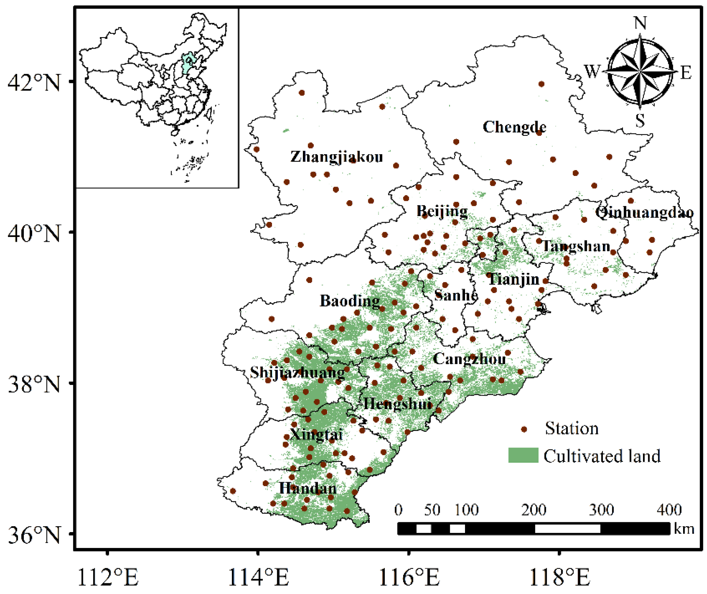
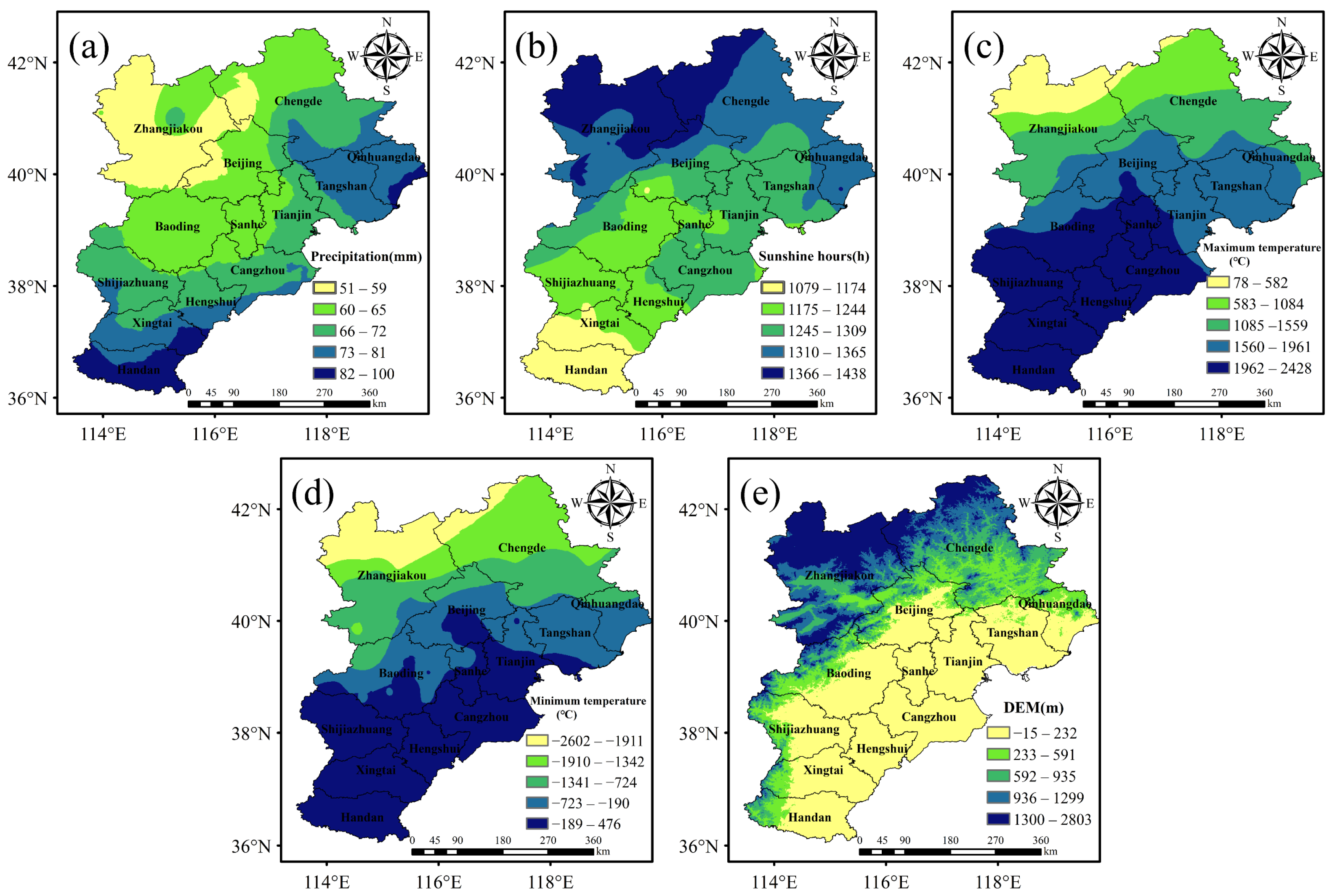
2.1. Study Area
2.2. Data
2.3. Methods
2.3.1. Improving the Moisture-Sensitive DSSAT Model
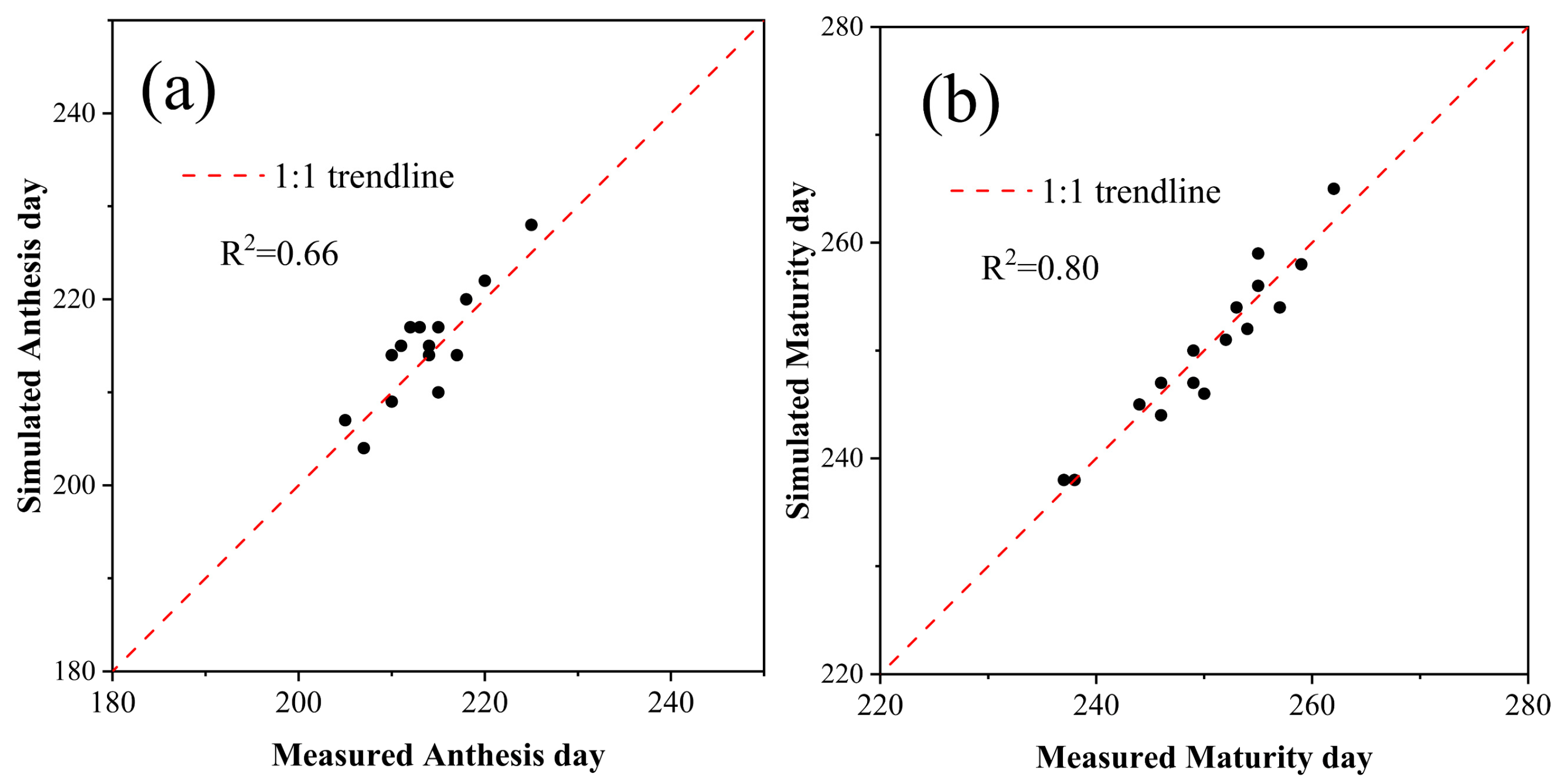
2.3.2. Model Accuracy Evaluation and Parameter Calibration
2.3.3. Drought Hazard Intensity Index
2.3.4. Gridded Drought Vulnerability Curves
2.3.5. Drought Risk Assessment
3. Results
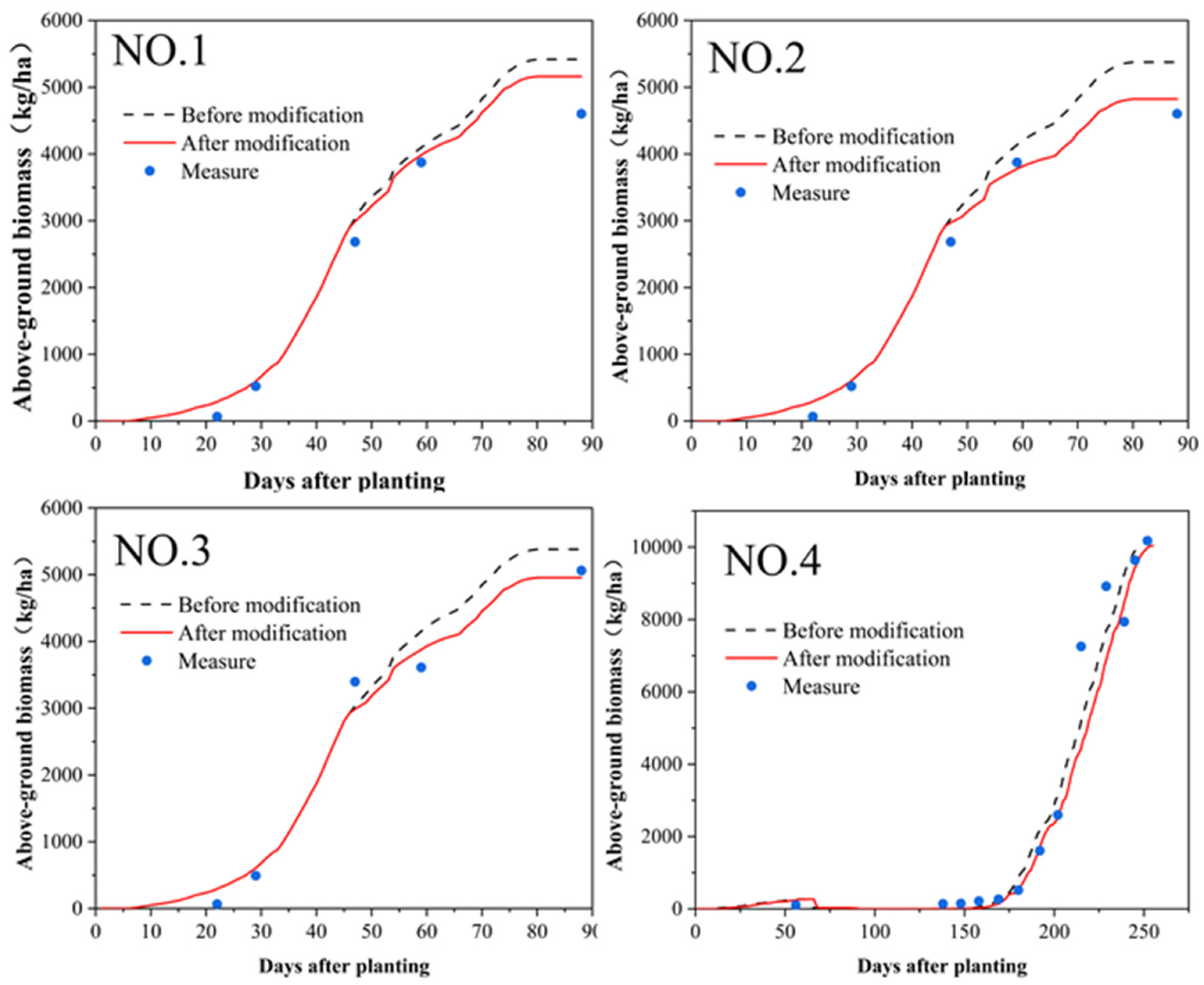
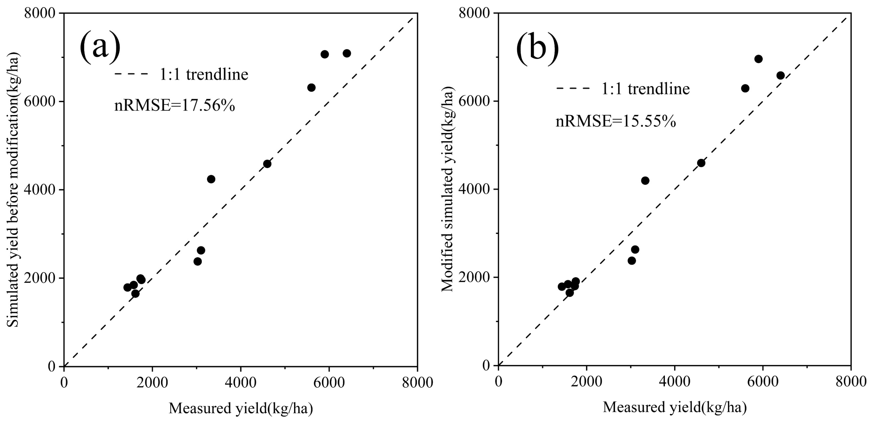
3.1. Model Accuracy Evaluation and Parameter Localization
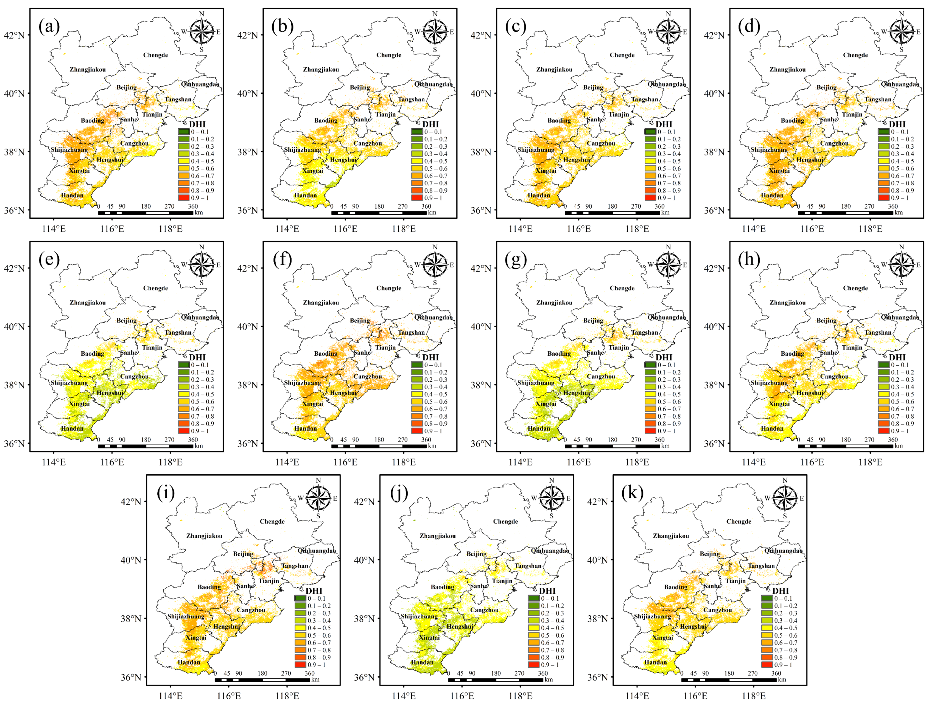
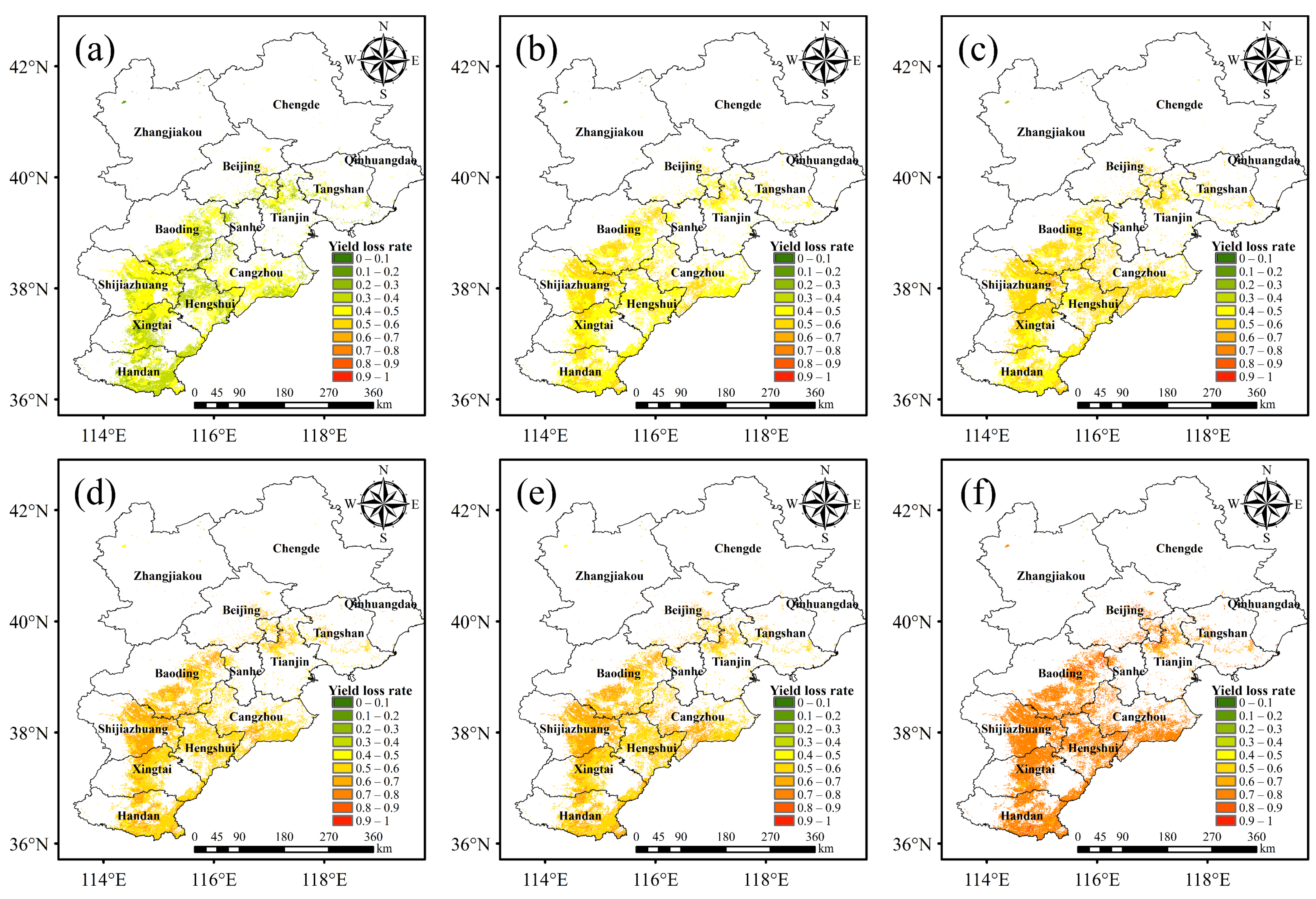
3.2. Drought Hazard Intensity Assessment
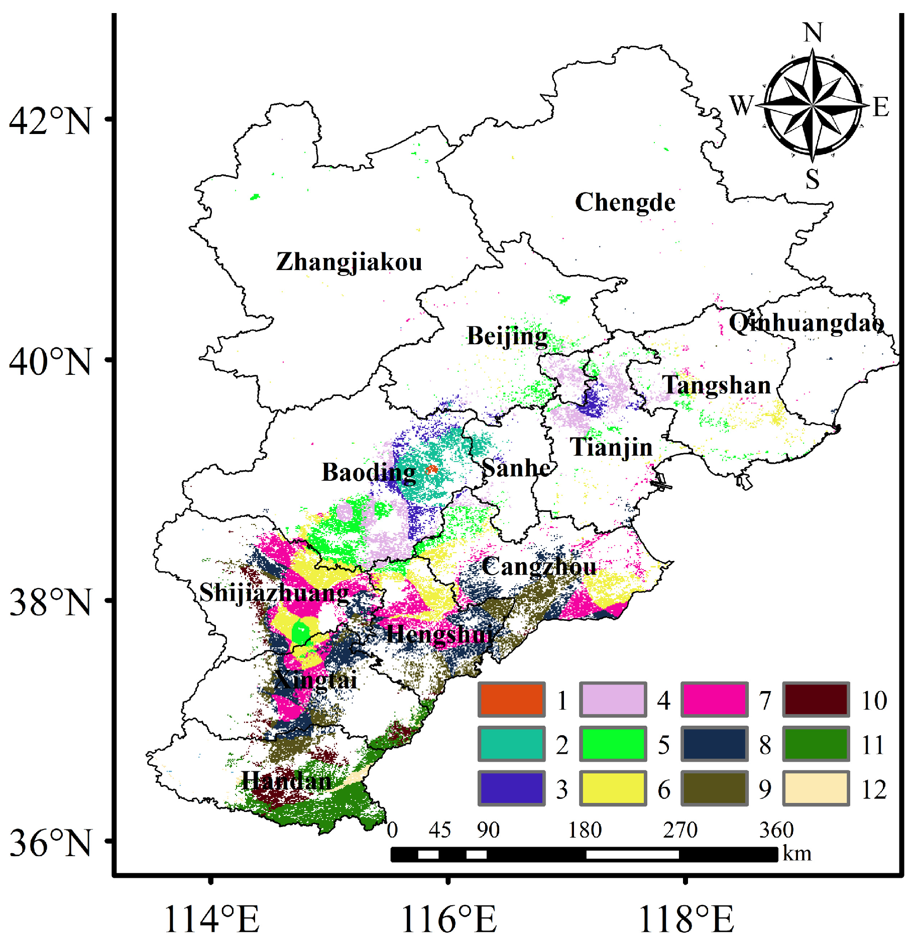
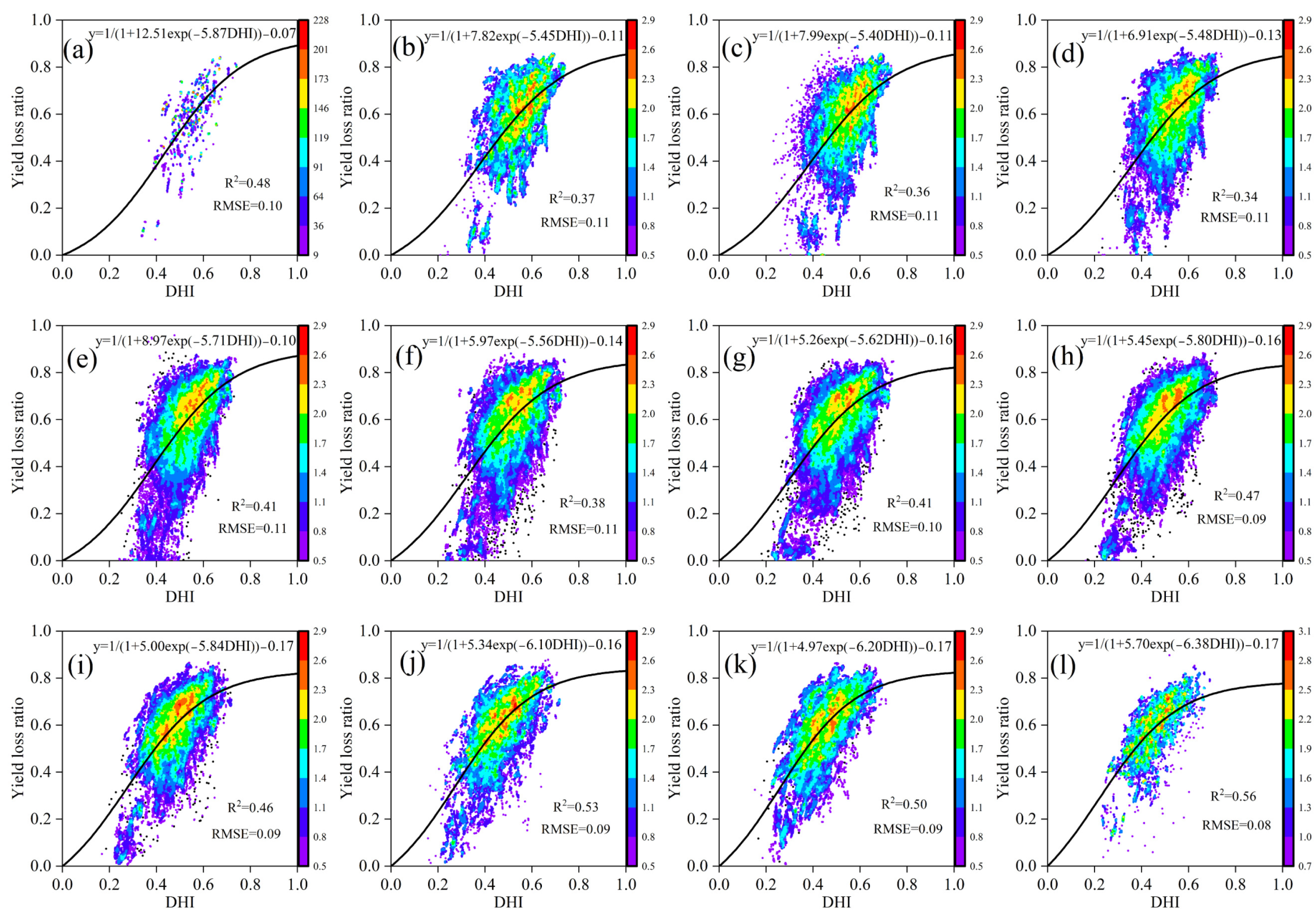
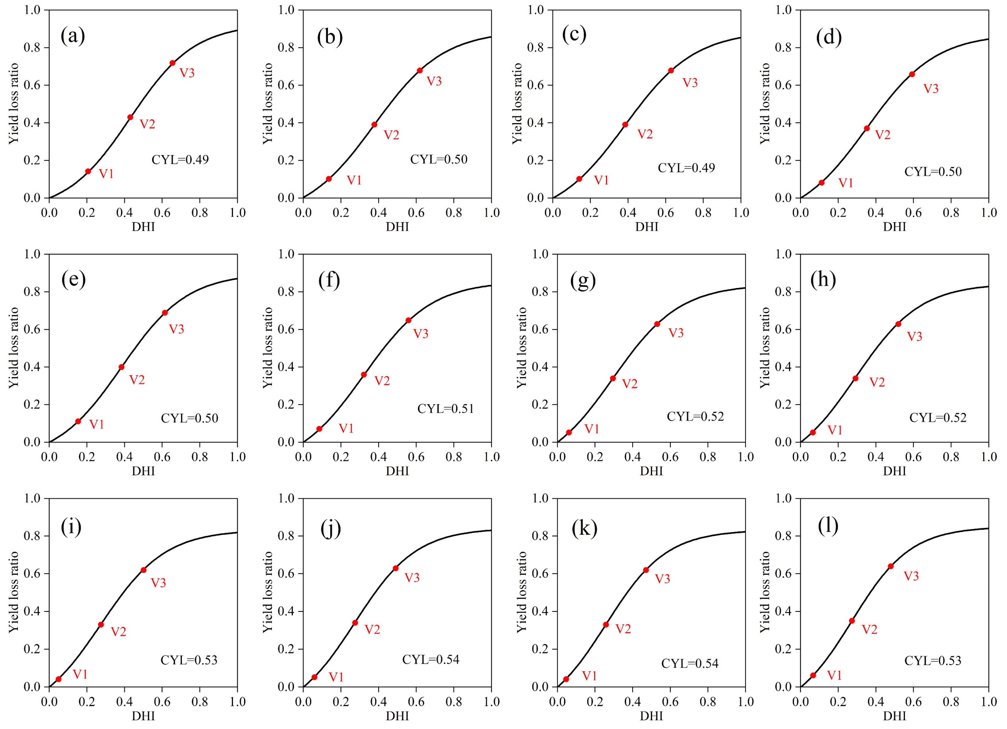
3.3. Gridded Vulnerability Curves and Characterization
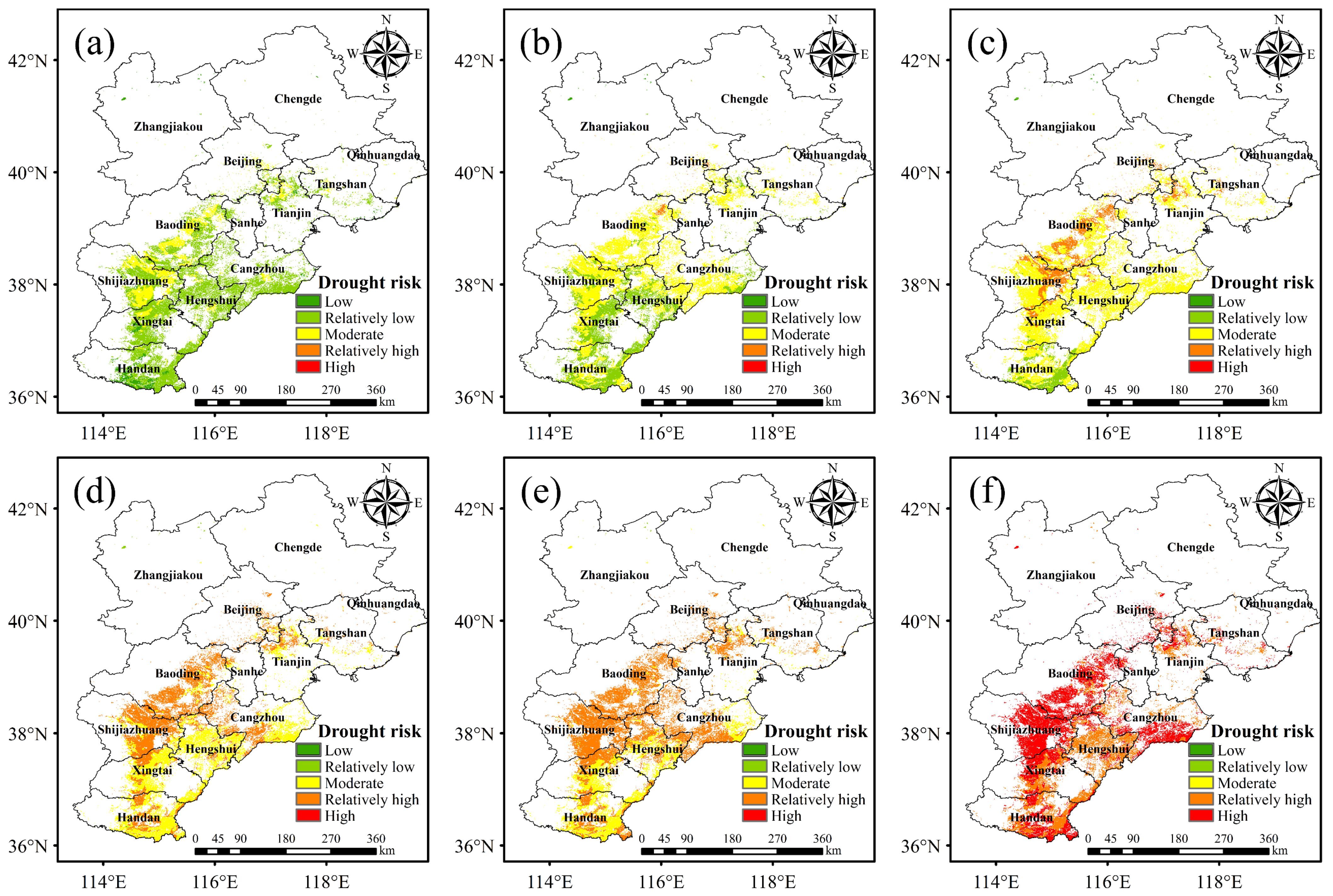
3.4. Drought Risk Assessment
4. Discussion
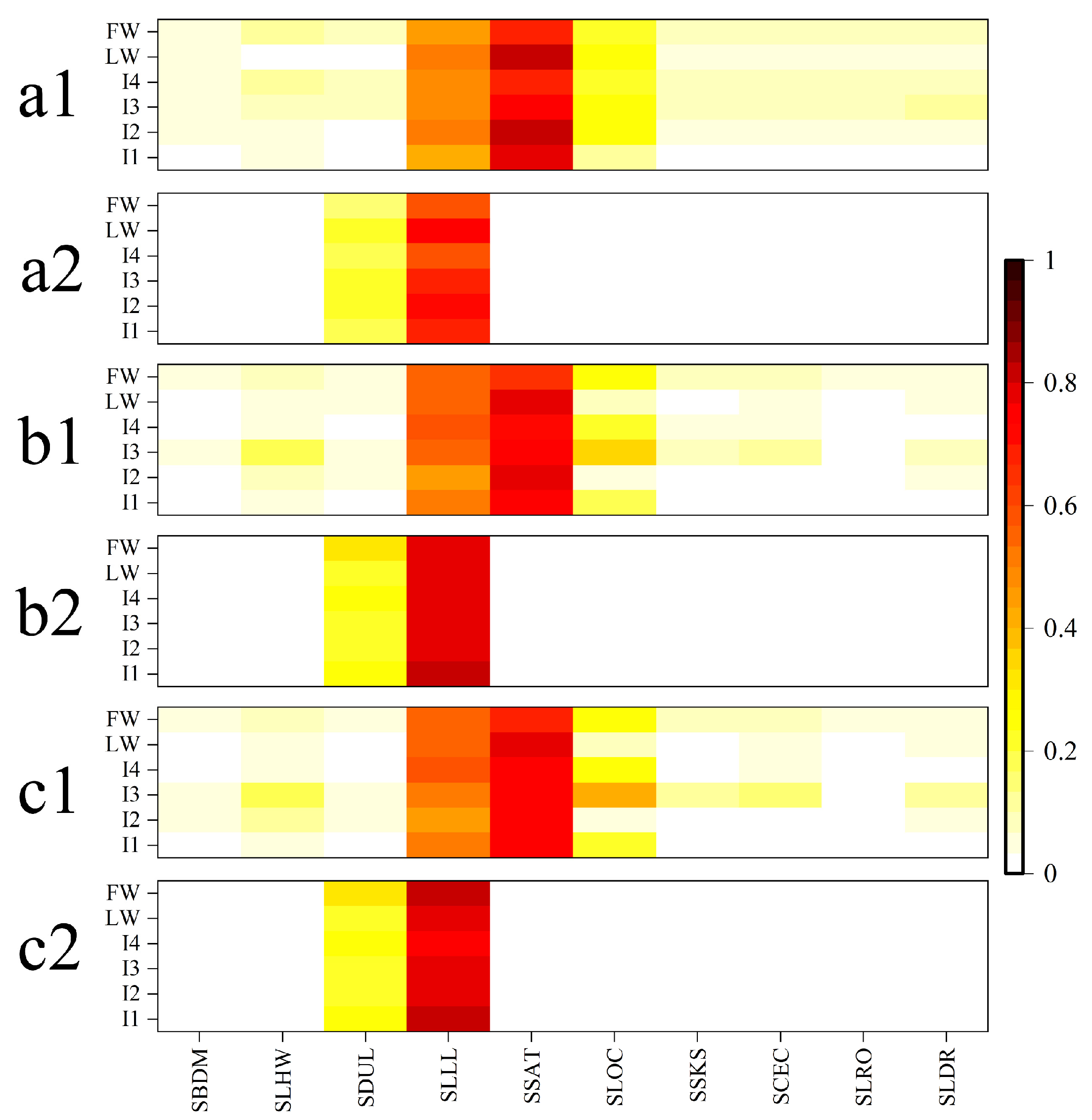
4.1. Sensitivity Analysis of Model Parameters
4.2. Advantages and Limitations
5. Conclusions
Author Contributions
Funding
Data Availability Statement
Acknowledgments
Conflicts of Interest
References
- Tan, C.; Yang, J.; Wang, X.; Qin, D.; Huang, B.; Chen, H. Drought disaster risks under CMIP5 RCP scenarios in Ningxia Hui Autonomous Region, China. Nat. Hazards 2020, 100, 909–931. [Google Scholar] [CrossRef]
- Yuan, X.; Zhou, Y.; Jin, J.; Wei, Y. Risk analysis for drought hazard in China: A case study in Huaibei Plain. Nat. Hazards 2013, 67, 879–900. [Google Scholar] [CrossRef]
- Zhang, Q.; Yao, Y.; Wang, Y.; Wang, S.; Wang, J.; Yang, J.; Wang, J.; Li, Y.; Shang, J.; Li, W. Characteristics of drought in Southern China under climatic warming, the risk, and countermeasures for prevention and control. Theor. Appl. Climatol. 2019, 136, 1157–1173. [Google Scholar] [CrossRef]
- Tsakiris, G. Drought Risk Assessment and Management. Water Resour. Manag. 2017, 31, 3083–3095. [Google Scholar] [CrossRef]
- Wei, Y.; Jin, J.; Jiang, S.; Ning, S.; Cui, Y.; Zhou, Y. Simulated Assessment of Summer Maize Drought Loss Sensitivity in Huaibei Plain, China. Agronomy 2019, 9, 78. [Google Scholar] [CrossRef] [Green Version]
- Kim, W.; Iizumi, T.; Nishimori, M. Global Patterns of Crop Production Losses Associated with Droughts from 1983 to 2009. J. Appl. Meteorol. Climatol. 2019, 58, 1233–1244. [Google Scholar] [CrossRef]
- González Tánago, I.; Urquijo, J.; Blauhut, V.; Villarroya, F.; De Stefano, L. Learning from experience: A systematic review of assessments of vulnerability to drought. Nat. Hazards 2016, 80, 951–973. [Google Scholar] [CrossRef]
- Singh, G. Salinity-related desertification and management strategies: Indian experience. Land Degrad. Dev. 2009, 20, 367–385. [Google Scholar] [CrossRef]
- Wang, Y.; Zhang, Q.; Yao, Y. Drought vulnerability assessment for maize in the semiarid region of northwestern China. Theor. Appl. Climatol. 2020, 140, 1207–1220. [Google Scholar] [CrossRef]
- Sivakumar, V.L.; Krishnappa, R.R.; Nallanathel, M. Drought vulnerability assessment and mapping using Multi-Criteria decision making (MCDM) and application of Analytic Hierarchy process (AHP) for Namakkal District, Tamilnadu, India. Mater. Today Proc. 2021, 43, 1592–1599. [Google Scholar] [CrossRef]
- Zhang, D.; Wang, G.; Zhou, H. Assessment on agricultural drought risk based on variable fuzzy sets model. Chin. Geogr. Sci. 2011, 21, 167–175. [Google Scholar] [CrossRef]
- Zhou, J.; Zhou, J.; Ye, H.; Ali, M.L.; Chen, P.; Nguyen, H.T. Yield estimation of soybean breeding lines under drought stress using unmanned aerial vehicle-based imagery and convolutional neural network. Biosyst. Eng. 2021, 204, 90–103. [Google Scholar] [CrossRef]
- An, J.; Li, W.; Li, M.; Cui, S.; Yue, H. Identification and Classification of Maize Drought Stress Using Deep Convolutional Neural Network. Symmetry 2019, 11, 256. [Google Scholar] [CrossRef] [Green Version]
- Jin, Z.; Zhuang, Q.; Tan, Z.; Dukes, J.S.; Zheng, B.; Melillo, J.M. Do maize models capture the impacts of heat and drought stresses on yield? Using algorithm ensembles to identify successful approaches. Glob. Change Biol. 2016, 22, 3112–3126. [Google Scholar] [CrossRef]
- Das Choudhury, S.; Saha, S.; Samal, A.; Mazis, A.; Awada, T. Drought stress prediction and propagation using time series modeling on multimodal plant image sequences. Front. Plant Sci. 2023, 14, 1003150. [Google Scholar] [CrossRef] [PubMed]
- Dai, M.; Huang, S.; Huang, Q.; Leng, G.; Guo, Y.; Wang, L.; Fang, W.; Li, P.; Zheng, X. Assessing agricultural drought risk and its dynamic evolution characteristics. Agric. Water Manag. 2020, 231, 106003. [Google Scholar] [CrossRef]
- Du, L.; Tian, Q.; Yu, T.; Meng, Q.; Jancso, T.; Udvardy, P.; Huang, Y. A comprehensive drought monitoring method integrating MODIS and TRMM data. Int. J. Appl. Earth Obs. Geoinf. 2013, 23, 245–253. [Google Scholar] [CrossRef]
- Thomas, T.; Jaiswal, R.K.; Galkate, R.; Nayak, P.C.; Ghosh, N.C. Drought indicators-based integrated assessment of drought vulnerability: A case study of Bundelkhand droughts in central India. Nat. Hazards 2016, 81, 1627–1652. [Google Scholar] [CrossRef]
- Kar, S.K.; Thomas, T.; Singh, R.M.; Patel, L. Integrated assessment of drought vulnerability using indicators for Dhasan basin in Bundelkhand region, Madhya Pradesh, India. Curr. Sci. 2018, 115, 338–346. [Google Scholar] [CrossRef]
- Zarafshani, K.; Maleki, T.; Keshavarz, M. Assessing the vulnerability of farm families towards drought in Kermanshah province, Iran. Geojournal 2020, 85, 823–836. [Google Scholar] [CrossRef]
- Zarafshani, K.; Sharafi, L.; Azadi, H.; Hosseininia, G.; De Maeyer, P.; Witlox, F. Drought vulnerability assessment: The case of wheat farmers in Western Iran. Glob. Planet. Chang. 2012, 98–99, 122–130. [Google Scholar] [CrossRef] [Green Version]
- Kim, H.; Park, J.; Yoo, J.; Kim, T. Assessment of drought hazard, vulnerability, and risk: A case study for administrative districts in South Korea. J. Hydro-Environ. Res. 2015, 9, 28–35. [Google Scholar] [CrossRef]
- Dabanli, I. Drought hazard, vulnerability, and risk assessment in Turkey. Arab. J. Geosci. 2018, 11, 538. [Google Scholar] [CrossRef]
- Tan, G.; Shibasaki, R. Global estimation of crop productivity and the impacts of global warming by GIS and EPIC integration. Ecol. Model. 2003, 168, 357–370. [Google Scholar] [CrossRef]
- Liu, J.G. A GIS-based tool for modelling large-scale crop-water relations. Environ. Model. Softw. 2009, 24, 411–422. [Google Scholar] [CrossRef]
- Liu, W.F.; Yang, H.; Folberth, C.; Wang, X.Y.; Luo, Q.Y.; Schulin, R. Global investigation of impacts of PET methods on simulating crop-water relations for maize. Agric. For. Meteorol. 2016, 221, 164–175. [Google Scholar] [CrossRef]
- Zhu, X.; Xu, K.; Liu, Y.; Guo, R.; Chen, L. Assessing the vulnerability and risk of maize to drought in China based on the AquaCrop model. Agric. Syst. 2021, 189, 103040. [Google Scholar] [CrossRef]
- Fawen, L.; Manjing, Z.; Yaoze, L. Quantitative research on drought loss sensitivity of summer maize based on AquaCrop model. Nat. Hazards 2022, 112, 1065–1084. [Google Scholar] [CrossRef]
- Keating, B.A.; Carberry, P.S.; Hammer, G.L.; Probert, M.E.; Robertson, M.J.; Holzworth, D.; Huth, N.I.; Hargreaves, J.N.G.; Meinke, H.; Hochman, Z.; et al. An overview of APSIM, a model designed for farming systems simulation. Eur. J. Agron. 2003, 18, 267–288. [Google Scholar] [CrossRef] [Green Version]
- Guo, H.; Wang, R.; Garfin, G.M.; Zhang, A.Y.; Lin, D.G.; Liang, Q.O.; Wang, J.A. Rice drought risk assessment under climate change: Based on physical vulnerability a quantitative assessment method. Sci. Total Environ. 2021, 751, 141481. [Google Scholar] [CrossRef]
- Wang, Z.; Jiang, J.; Ma, Q. The drought risk of maize in the farming-pastoral ecotone in Northern China based on physical vulnerability assessment. Nat. Hazards Earth Syst. Sci. 2016, 16, 2697–2711. [Google Scholar] [CrossRef] [Green Version]
- Li, R.; Tsunekawa, A.; Tsubo, M. Assessment of agricultural drought in rainfed cereal production areas of northern China. Theor. Appl. Climatol. 2017, 127, 597–609. [Google Scholar] [CrossRef]
- Wei, Y.; Jin, J.; Cui, Y.; Ning, S.; Fei, Z.; Wu, C.; Zhou, Y.; Zhang, L.; Liu, L.; Tong, F. Quantitative assessment of soybean drought risk in Bengbu city based on disaster loss risk curve and DSSAT. Int. J. Disaster Risk Reduct. 2021, 56, 102126. [Google Scholar] [CrossRef]
- Yassi, A.; Syaiful, S.A.; Ruslan, A.; Ridwan, I.; Andari, G. Simulation and production of soybean plant growth (Glycine max (L) Merrill) using the DSSAT model with different scenarios of water supply and compost. IOP Conf. Ser. Earth Environ. Sci. 2019, 343, 12014. [Google Scholar] [CrossRef]
- Yao, N.; Li, Y.; Liu, Q.; Zhang, S.; Chen, X.; Ji, Y.; Liu, F.; Pulatov, A.; Feng, P. Response of wheat and maize growth-yields to meteorological and agricultural droughts based on standardized precipitation evapotranspiration indexes and soil moisture deficit indexes. Agric. Water Manag. 2022, 266, 107566. [Google Scholar] [CrossRef]
- Paff, K.; Asseng, S. A Crop Simulation Model for Tef (Eragrostis tef (Zucc.) Trotter). Agronomy 2019, 9, 817. [Google Scholar] [CrossRef] [Green Version]
- Chen, X.G.; Li, Y.; Yao, N.; Liu, D.L.; Javed, T.; Liu, C.C.; Liu, F.G. Impacts of multi-timescale SPEI and SMDI variations on winter wheat yields. Agric. Syst. 2020, 185, 102955. [Google Scholar] [CrossRef]
- Shen, H.; Chen, Y.; Wang, Y.; Xing, X.; Ma, X. Evaluation of the Potential Effects of Drought on Summer Maize Yield in the Western Guanzhong Plain, China. Agronomy 2020, 10, 1095. [Google Scholar] [CrossRef]
- Hu, Y.; Liu, Y.; Tang, H.; Xu, Y.; Pan, J. Contribution of Drought to Potential Crop Yield Reduction in a Wheat-Maize Rotation Region in the North China Plain. J. Integr. Agric. 2014, 13, 1509–1519. [Google Scholar] [CrossRef]
- Li, Y.; Huang, H.; Ju, H.; Lin, E.; Xiong, W.; Han, X.; Wang, H.; Peng, Z.; Wang, Y.; Xu, J.; et al. Assessing vulnerability and adaptive capacity to potential drought for winter-wheat under the RCP 8.5 scenario in the Huang-Huai-Hai Plain. Agric. Ecosyst. Environ. 2015, 209, 125–131. [Google Scholar] [CrossRef]
- Jia, H.; Wang, J.; Cao, C.; Pan, D.; Shi, P. Maize drought disaster risk assessment of China based on EPIC model. Int. J. Digit. Earth 2012, 5, 488–515. [Google Scholar] [CrossRef]
- Vannoppen, A.; Gobin, A. Estimating Farm Wheat Yields from NDVI and Meteorological Data. Agronomy. 2021, 11, 946. [Google Scholar] [CrossRef]
- Tuvdendorj, B.; Zeng, H.; Wu, B.; Elnashar, A.; Zhang, M.; Tian, F.; Nabil, M.; Nanzad, L.; Bulkhbai, A.; Natsagdorj, N. Performance and the Optimal Integration of Sentinel-1/2 Time-Series Features for Crop Classification in Northern Mongolia. Remote Sens. 2022, 14, 1830. [Google Scholar] [CrossRef]
- Zhang, J.; He, Y.; Lin, Y.; Liu, P.; Zhou, X.; Huang, Y. Machine Learning-Based Spectral Library for Crop Classification and Status Monitoring. Agronomy 2019, 9, 496. [Google Scholar] [CrossRef] [Green Version]
- Wang, T.; Lv, C.; Yu, B. Assessing the Potential Productivity of Winter Wheat Using WOFOST in the Beijing-Tianjin-Hebei Region. J. Nat. Resour. 2010, 25, 475–487. (In Chinese) [Google Scholar]
- Li, H.; Lian, Y.; Wang, X.; Ma, W.; Zhao, L. Solar constant values for estimating solar radiation. Energy 2011, 36, 1785–1789. [Google Scholar] [CrossRef]
- Wei, S.; Dai, Y.; Liu, B.; Zhu, A.; Duan, Q.; Wu, L.; Ji, D.; Ye, A.; Yuan, H.; Zhang, Q.; et al. A China Dataset of Soil Properties for Land Surface Modeling; National Tibetan Plateau Data Center: Beijing, China, 2021. (In Chinese) [Google Scholar]
- Dai, Y.; Shangguan, W.; Duan, Q.; Liu, B.; Fu, S.; Niu, G. Development of a China Dataset of Soil Hydraulic Parameters Using Pedotransfer Functions for Land Surface Modeling. J. Hydrometeorol. 2013, 14, 869–887. [Google Scholar] [CrossRef] [Green Version]
- Shangguan, W.; Dai, Y. A China Dataset of Soil Hydraulic Parameters Pedotransfer Functions for Land Surface Modeling (1980); National Tibetan Plateau Data Center: Beijing, China, 2022. (In Chinese) [Google Scholar]
- Shen, H.; Gao, Y.; Guo, F.; Wang, Y.; Ma, X. A modified DSSAT-CERES model for simulating summer maize growth under film mulching. Agron. J. 2021, 113, 4819–4831. [Google Scholar] [CrossRef]
- Timsina, J.; Humphreys, E. Performance of CERES-Rice and CERES-Wheat models in rice-wheat systems: A review. Agric. Syst. 2006, 90, 5–31. [Google Scholar] [CrossRef]
- Jones, J.W.; Hoogenboom, G.; Porter, C.H.; Boote, K.J.; Batchelor, W.D.; Hunt, L.A.; Wilkens, P.W.; Singh, U.; Gijsman, A.J.; Ritchie, J.T. The DSSAT cropping system model. Eur. J. Agron. 2003, 18, 235–265. [Google Scholar] [CrossRef]
- Camargo, G.G.T.; Kemanian, A.R. Six crop models differ in their simulation of water uptake. Agric. For. Meteorol. 2016, 220, 116–129. [Google Scholar] [CrossRef] [Green Version]
- Zhang, Q.; Zhang, J.; Wang, C.; Cui, L.; Yan, D. Risk early warning of maize drought disaster in Northwestern Liaoning Province, China. Nat. Hazards 2014, 72, 701–710. [Google Scholar] [CrossRef]
- Geerts, S.; Raes, D.; Garcia, M.; Taboada, C.; Miranda, R.; Cusicanqui, J.; Mhizha, T.; Vacher, J. Modeling the potential for closing quinoa yield gaps under varying water availability in the Bolivian Altiplano. Agric. Water Manag. 2009, 96, 1652–1658. [Google Scholar] [CrossRef]
- Wu, Y.; Guo, H.; Zhang, A.; Wang, J. Establishment and characteristics analysis of a crop-drought vulnerability curve: A case study of European winter wheat. Nat. Hazards Earth Syst. Sci. 2021, 21, 1209–1228. [Google Scholar] [CrossRef]
- Guo, H.; Zhang, X.; Lian, F.; Gao, Y.; Lin, D.; Wang, J.A. Drought Risk Assessment Based on Vulnerability Surfaces: A Case Study of Maize. Sustainability 2016, 8, 813. [Google Scholar] [CrossRef] [Green Version]
- Ma, H.; Malone, R.W.; Jiang, T.; Yao, N.; Chen, S.; Song, L.; Feng, H.; Yu, Q.; He, J. Estimating crop genetic parameters for DSSAT with modified PEST software. Eur. J. Agron. 2020, 115, 126017. [Google Scholar] [CrossRef]
- Raymundo; Sexton-Bowser, S.; Ciampitti, I.A.; Morris, G.P. Crop modeling defines opportunities and challenges for drought escape, water capture, and yield increase using chilling-tolerant sorghum. Plant Direct. 2021, 5, e349. [Google Scholar] [CrossRef]
- Varella, H.; Guérif, M.; Buis, S. Global sensitivity analysis measures the quality of parameter estimation: The case of soil parameters and a crop model. Environ. Model. Softw. 2010, 25, 310–319. [Google Scholar] [CrossRef]
- Ma, H.; Wang, J.; Liu, T.; Guo, Y.; Zhou, Y.; Yang, T.; Zhang, W.; Sun, C. Time series global sensitivity analysis of genetic parameters of CERES-maize model under water stresses at different growth stages. Agric. Water Manag. 2023, 275, 108027. [Google Scholar] [CrossRef]
- Li, Z.; Jin, X.; Liu, H.; Xu, X.; Wang, J. Global sensitivity analysis of wheat grain yield and quality and the related process variables from the DSSAT-CERES model based on the extended Fourier Amplitude Sensitivity Test method. J. Integr. Agric. 2019, 18, 1547–1561. [Google Scholar] [CrossRef]
- Kassie, B.T.; Asseng, S.; Rotter, R.P.; Hengsdijk, H.; Ruane, A.C.; Van Ittersum, M.K. Exploring climate change impacts and adaptation options for maize production in the Central Rift Valley of Ethiopia using different climate change scenarios and crop models. Clim. Chang. 2015, 129, 145–158. [Google Scholar] [CrossRef]
- He, W.; Yang, J.Y.; Zhou, W.; Drury, C.F.; Yang, X.M.; Reynolds, W.D.; Wang, H.; He, P.; Li, Z.T. Sensitivity analysis of crop yields, soil water contents and nitrogen leaching to precipitation, management practices and soil hydraulic properties in semi-arid and humid regions of Canada using the DSSAT model. Nutr. Cycl. Agroecosyst. 2016, 106, 201–215. [Google Scholar] [CrossRef]
- DeJonge, K.C.; Ascough, J.C.; Ahmadi, M.; Andales, A.A.; Arabi, M. Global sensitivity and uncertainty analysis of a dynamic agroecosystem model under different irrigation treatments. Ecol. Model. 2012, 231, 113–125. [Google Scholar] [CrossRef]
- Zhuo, W.; Huang, H.; Gao, X.; Li, X.; Huang, J. An Improved Approach of Winter Wheat Yield Estimation by Jointly Assimilating Remotely Sensed Leaf Area Index and Soil Moisture into the WOFOST Model. Remote Sens. 2023, 15, 1825. [Google Scholar] [CrossRef]
- Itoh, Y.; Bröcker, M.J.; Sekine, S.; Söll, D.; Yokoyama, S. Dimer-Dimer Interaction of the Bacterial Selenocysteine Synthase SelA Promotes Functional Active-Site Formation and Catalytic Specificity. J. Mol. Biol. 2014, 426, 1723–1735. [Google Scholar] [CrossRef] [Green Version]
- Geng, S.M.; Yan, D.H.; Yang, Z.Y.; Zhang, Z.B.; Yang, M.J.; Kan, G.Y. Characteristics Analysis of Summer Maize Yield Loss Caused by Drought Stress in the Northern Huaihe Plain, China. Irrig. Drain. 2018, 67, 251–268. [Google Scholar] [CrossRef]
- Ran, H.; Kang, S.; Hu, X.; Li, S.; Wang, W.; Liu, F. Capability of a solar energy-driven crop model for simulating water consumption and yield of maize and its comparison with a water-driven crop model. Agric. For. Meteorol. 2020, 287, 107955. [Google Scholar] [CrossRef]


| The Starting Point of Rapid Loss Growth (V1) | The Inflection Point of Rapid Loss Growth (V2) | The End Point of Rapid Loss Growth (V3) | |
|---|---|---|---|
| DHI | |||
| YL |
| Risk Index | ≤0.09 | 0.09~0.18 | 0.18~0.28 | 0.28~0.46 | ≥0.46 |
|---|---|---|---|---|---|
| Risk level | low | relatively low | moderate | relatively high | high |
| Trial Number | Before Modification (%) | After Modification (%) | Error Reduction (%) |
|---|---|---|---|
| 1 | 17.98 | 13.08 | 4.89 |
| 2 | 12.21 | 10.60 | 1.61 |
| 3 | 13.61 | 9.94 | 3.67 |
| 4 | 20.94 | 17.91 | 3.03 |
| Factor | DHI |
|---|---|
| Precipitation | −0.66 ** |
| Sunshine hours | 0.31 ** |
| Daily maximum temperature | −0.37 ** |
| Daily minimum temperature | −0.49 ** |
| Number | Count | Proportion (%) | Number | Count | Proportion (%) |
|---|---|---|---|---|---|
| 1 | 69 | 0.14 | 7 | 7823 | 16.30 |
| 2 | 2521 | 5.25 | 8 | 7647 | 15.93 |
| 3 | 2019 | 4.21 | 9 | 5076 | 10.57 |
| 4 | 3932 | 8.19 | 10 | 2181 | 4.54 |
| 5 | 4632 | 9.65 | 11 | 5133 | 10.69 |
| 6 | 6519 | 13.58 | 12 | 452 | 0.94 |
| Input Parameters | Meaning | Range of Values |
|---|---|---|
| SBDM | Bulk density | (0.8, 1.5) |
| SLHW | PH | (5.4, 9.5) |
| SDUL | Drained upper limit | (0.25, 0.34) |
| SLLL | Lower limit of soil drainage | (0.1, 0.24) |
| SSAT | Soil saturation | (0.35, 0.6) |
| SLOC | Organic carbon content | (0.4, 5.0) |
| SSKS | Soil saturation hydraulic conductivity | (0.1, 21.0) |
| SCEC | Cation exchange capacity | (1, 30) |
| SLRO | Runoff curve number | (61, 94) |
| SLDR | Drainage rate | (0.01, 0.85) |
| Number | Overwintering Period | Greening Period | Plucking Period | Spike Period | Grouting Period |
|---|---|---|---|---|---|
| 11–15 | 3–5 | 4–20 | 5–5 | 5–20 | |
| I1 | 0 | 0 | 50 | 50 | 50 |
| I2 | 50 | 0 | 0 | 50 | 50 |
| I3 | 50 | 50 | 0 | 0 | 50 |
| I4 | 50 | 50 | 50 | 0 | 0 |
| LW | 0 | 0 | 0 | 0 | 0 |
| FW | 50 | 50 | 50 | 50 | 50 |
Disclaimer/Publisher’s Note: The statements, opinions and data contained in all publications are solely those of the individual author(s) and contributor(s) and not of MDPI and/or the editor(s). MDPI and/or the editor(s) disclaim responsibility for any injury to people or property resulting from any ideas, methods, instructions or products referred to in the content. |
© 2023 by the authors. Licensee MDPI, Basel, Switzerland. This article is an open access article distributed under the terms and conditions of the Creative Commons Attribution (CC BY) license (https://creativecommons.org/licenses/by/4.0/).
Share and Cite
Yang, H.; Li, Z.; Du, Q.; Duan, Z. Winter Wheat Drought Risk Assessment by Coupling Improved Moisture-Sensitive Crop Model and Gridded Vulnerability Curve. Remote Sens. 2023, 15, 3197. https://doi.org/10.3390/rs15123197
Yang H, Li Z, Du Q, Duan Z. Winter Wheat Drought Risk Assessment by Coupling Improved Moisture-Sensitive Crop Model and Gridded Vulnerability Curve. Remote Sensing. 2023; 15(12):3197. https://doi.org/10.3390/rs15123197
Chicago/Turabian StyleYang, Haibo, Zenglan Li, Qingying Du, and Zheng Duan. 2023. "Winter Wheat Drought Risk Assessment by Coupling Improved Moisture-Sensitive Crop Model and Gridded Vulnerability Curve" Remote Sensing 15, no. 12: 3197. https://doi.org/10.3390/rs15123197