Article

Monitoring Forest Cover Dynamics Using Orthophotos and Satellite Imagery

1
Department of Geography, Tourism and Territorial Planning, Faculty of Geography, Tourism and Sport, The Territorial Studies and Analyses Centre (CSAT), University of Oradea, 410087 Oradea, Romania
2
Institute of Socio-Economic Geography and Spatial Management, University of Gdansk, 80309 Gdansk, Poland
3
Faculty of Geography, Babes-Bolyai University, 400006 Cluj-Napoca, Romania
4
Faculty of Resources and Environmental Science, Hubei University, Wuhan 430062, China
5
Faculty of Economics and Business, John von Neumann University, 6000 Kecskemet, Hungary
6
Institute of Rural Development and Sustainable Economy, Hungarian University of Agriculture and Life Sciences, 2100 Godollo, Hungary
*
Author to whom correspondence should be addressed.
These authors contributed equally to this work.
Remote Sens. 2023, 15(12), 3168; https://doi.org/10.3390/rs15123168
Submission received: 12 May 2023 / Revised: 16 June 2023 / Accepted: 16 June 2023 / Published: 18 June 2023
(This article belongs to the Special Issue Image Analysis for Forest Environmental Monitoring)

Abstract

:
The assessment of changes in forest coverage is crucial for managing protected forest areas, particularly in the face of climate change. This study monitored forest cover dynamics in a 6535 ha mountain area located in north-west Romania as part of the Apuseni Natural Park from 2003 to 2019. Two approaches were used: vectorization from orthophotos and Google Earth images (in 2003, 2005, 2009, 2012, 2014, 2016, 2017, and 2019) and satellite imagery (Landsat 5 TM, 7 ETM, and 8 OLI) pre-processed to Surface Reflectance (SR) format from the same years. We employed four standard classifiers: Support Vector Machine (SVM), Random Forest (RF), Maximum Likelihood Classification (MLC), Spectral Angle Mapper (SAM), and three combined methods: Linear Spectral Unmixing (LSU) with Natural Breaks (NB), Otsu Method (OM) and SVM, to extract and classify forest areas. Our study had two objectives: (1) to accurately assess changes in forest cover over a 17-year period and (2) to determine the most efficient methods for extracting and classifying forest areas. We validated the results using performance metrics that quantify both thematic and spatial accuracy. Our results indicate a 9% loss of forest cover in the study area, representing 577 ha with an average decrease ratio of 33.9 ha/year−1. Of all the methods used, SVM produced the best results (with an average score of 88% for Overall Quality (OQ)), followed by RF (with a mean value of 86% for OQ).

1. Introduction

The importance of temperate forest ecosystems in the carbon cycle, as well as their aesthetic, social, and anti-erosion, or hydrological control functions, are well-established [1,2,3]. However, the long-term effects of climate change on these ecosystems, which have already begun to affect their functionality in various ways [4,5], remain poorly understood. The observed and predicted increases in temperature in temperate areas of Central and Eastern Europe since 1950 [6] have led to changes in the phenology of temperate forests, with an extension in the period of growth being positively appreciated for biomass production and carbon sequestration rates based on several studies [4,5,7,8]. However, the increase in periods with extreme temperatures, droughts [9], and heavy precipitation events has also led to an increase in natural disturbances specific to European temperate forests, such as windthrow, bark beetle infestation (Ips typographus (L.)), and root rot (Heterobasidium annosum, e.g.) [10]. Senf and Seidl [11] reported that of the 227 million hectares of forests in Europe [12], 17% were disturbed between 1986 and 2016 due to natural and/or anthropogenic causes. Similarly, Forzieri et al. [13] quantified the vulnerability of European forests to fires, windthrows, and insect outbreaks and estimated that 33.4 billion tonnes of forest biomass could be affected by these disturbances. The results of Wang et al.’s [3] analysis of the effects of climate change, CO2 increase in the atmosphere, and nitrogen deposition on aboveground net primary production in a temperate forest suggest that the total negative effect induced by climate change will not be fully compensated by the total positive effect.
Remote sensing and GIS (geographic information system) techniques are widely used in the scientific community to monitor and assess forest ecosystems quantitatively and qualitatively [14,15]. These efforts include studying the spatial extension and alterations of forest vegetation at global, regional, and local levels, with clear implications for biodiversity decline [16,17]. In recent decades, research in this area has diversified from identifying and extracting forest vegetation classes [18,19,20,21,22,23] or tree species [24,25,26,27,28,29] to analyzing the spatial-temporal evolution of forested areas based on various ranges of satellite images [30,31,32,33,34,35,36,37,38,39,40,41,42]. Many studies focus on comparative analyses of methods for extracting, classifying, and quantifying vegetation, including forests, and some combined this with time series imagery.
Huang et al. [43] tested Support Vector Machines (SVM), Maximum Likelihood Classification (MLC), Neural Network (ANN), and Decision Tree (DT) algorithms on a modified Landsat TM (1985) image from eastern Maryland, USA, with six land coverage classes (closed forest, open forest, woodland, non-forest land, land-water mix, and water). They evaluated the classifiers’ performance based on thematic accuracy and highlighted SVM’s results, depending on the kernel type used. Shafri et al. [44] tested MLC, Spectral Angle Mapper (SAM), ANN, and DT to map Malaysian tropical forests using hyperspectral data and highlighted MLC’s superior performance in conditions of maximum biotic heterogeneity. Otukei and Blaschke [45] used DT, SVM, and MLC to assess land cover changes using two Landsat scenes (5 TM from 1986 and 7 ETM+ from 2001) in eastern Uganda and found that all methods were effective with acceptable accuracy, with slight advantage for DT.
Comparative research in this field includes studying the behavior of different combinations of entry data used in classifications, the behavior of classifiers with varying training sample sizes, and the performance of combinations between classification methods. For example, Forkuor et al. [46] used SVM, Random Forest (RF), and Stochastic Gradient Boosting (SGB) to test different combinations of Landsat 8 OLI and Sentinel-2 images for land-use and land-cover mapping in Burkina Faso. They found that using the two Red Edge bands from Sentinel-2 improved land-use land-cover (LULC) mapping and SGB outperformed SVM and RF in overall performance. Thanh Noi and Kappas [47] compared RF, k-Nearest Neighbor (kNN), and SVM for six Land Use Land Cover (LULC) types, including forest, using 14 different training sample sizes in the Red River Delta of Vietnam based on a Sentinel-2 image. Their study emphasized the need to adjust parameters for the compared classifiers and indicated SVM’s lower sensitivity to training sample sizes. Adugna et al. [48] tested SVM and RF for regional land cover mapping in East Africa based on FY-3C scenes with a resolution of 1 km. Nguyen et al. [49] used 446 Sentinel-2 images from 2017 and 2018 to map LULC, including tropical forest classes, in Dak Nong, Vietnam, using four classification methods (Multinomial Logistic Regression—MLR, Improved kNN, RF, and SVM) tested for four time sequences (wet season, dry season, the entire year 2017, and a combination of wet-dry seasons). Ruggeri et al. [50] combined Linear Spectral Unmixing (LSU) with Object-Based Image Analysis (OBIA) and Iterative Self-Organizing Data Analysis Technique (ISODATA) with OBIA for land cover mapping in high mountain areas in Colombia, using a classification scheme adapted from CORINE Land Cover (CLC), which includes forest classes. Dabija et al. [51] used Random Forests and SVM on Sentinel-2 and Landsat 8 OLI satellite images covering three regions from three European Union countries to test CLC classes, including forest classes such as broad-leaved and coniferous forests.
All of the studies presented aim to identify the classification methods with the highest efficiency for the given entry data and intended purposes. Our study seeks to evaluate the dynamics of forest cover in a 6535 ha mountainous area located in NW Romania over a 17-year period (2003–2019) using GIS techniques, as well as extraction and classification methods for forest vegetation on multispectral scenes. Specifically, we employed LSU combined with Natural Breaks (NB), Otsu Method (OM), and SVM, SAM, SVM, RF, and MLC, respectively. Our primary objectives were to determine the exact loss/growth of forest cover in the area during the given time period and to validate the best method or methods for extracting/classifying forest cover from satellite data, using GIS data as the reference basis. In other words, we aimed to identify which methods, applied to medium-resolution satellite scenes, produced results closer to the GIS data obtained from high-resolution images. To assess the accuracy of the results, we used two types of entry data: continuous data and discrete data [52].

2. Materials and Methods
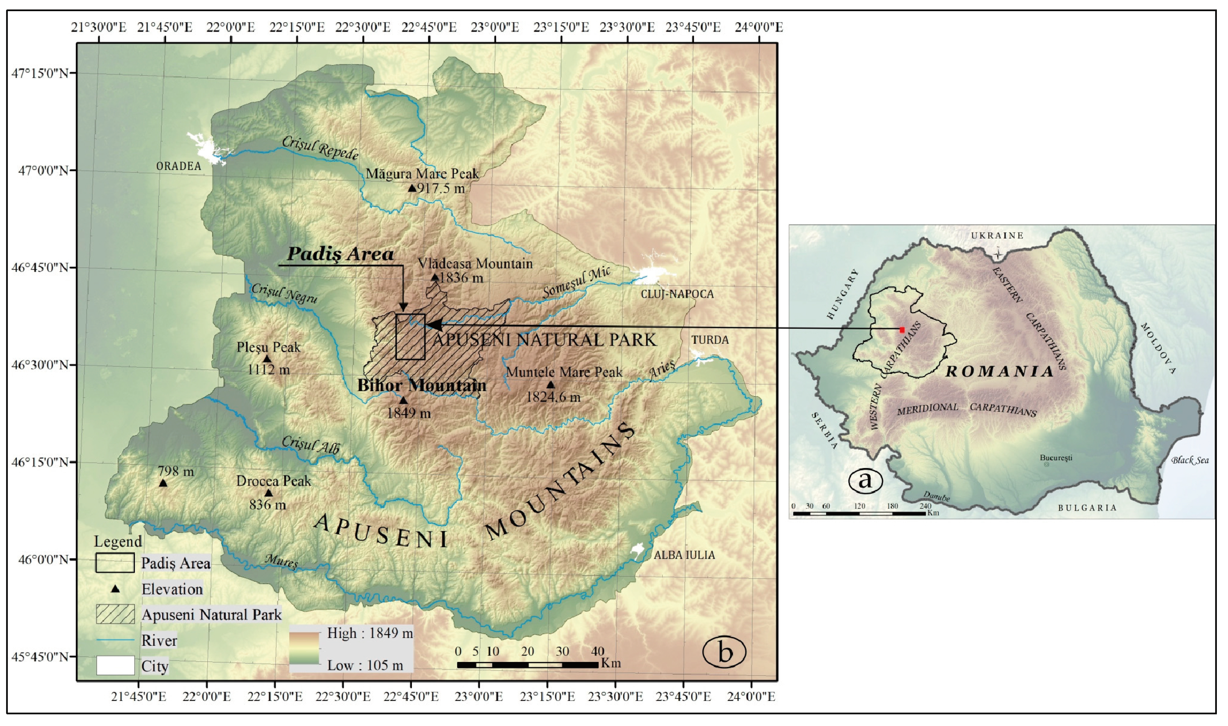
2.1. Study Area

The study area, Padiș, is located in the north of the Bihor massif in the Apuseni Mountains, which are part of the Romanian Western Carpathians (Figure 1). This area encompasses over 90% of one of the most complex and spectacular karst morphosystems in Romania, including the closed basin Padiș-Cetățile Ponorului, an endorheic area of 36 km2 with underground drainage that resembles a karst plateau situated at an altitude of 1250–1280 m [53], the Someșului Cald-Cetatea Rădesei gorge sector, and Galbenei gorges. Padiș falls administratively under Bihor County, and ecological management is provided by the Apuseni Natural Park, a protected area of national interest of category V IUCN, established through Ministerial Order no. 7/1990 and reconfirmed by Law no. 5/2000.
The dominant vegetation in the area consists of coniferous forests (Norway spruce—Picea abies), broad-leaved forests (European beech—Fagus silvatica), and, to some extent, mixed forests (beech and spruce) [53,54]. Vegetation inversions occur frequently due to microclimatic conditions, with spruce growing in deep karst depressions. Grasslands (meadows) composed mainly of grass species also occupy significant areas within the karst plateaus. In some places, intensive grazing and woodland exploitation have led to a decrease in the density of herbaceous vegetation cover, resulting in decay. The Forest CLC classes (2000–2018) [55] that cover the area include coniferous forest, broad-leaved forest, and mixed forest. As a protected area, the anthropogenic activities that put pressure on these natural components are related to wood exploitation, animal husbandry, and intensive tourism during the spring-summer season.

2.2. Data Acquisition and Pre-Processing
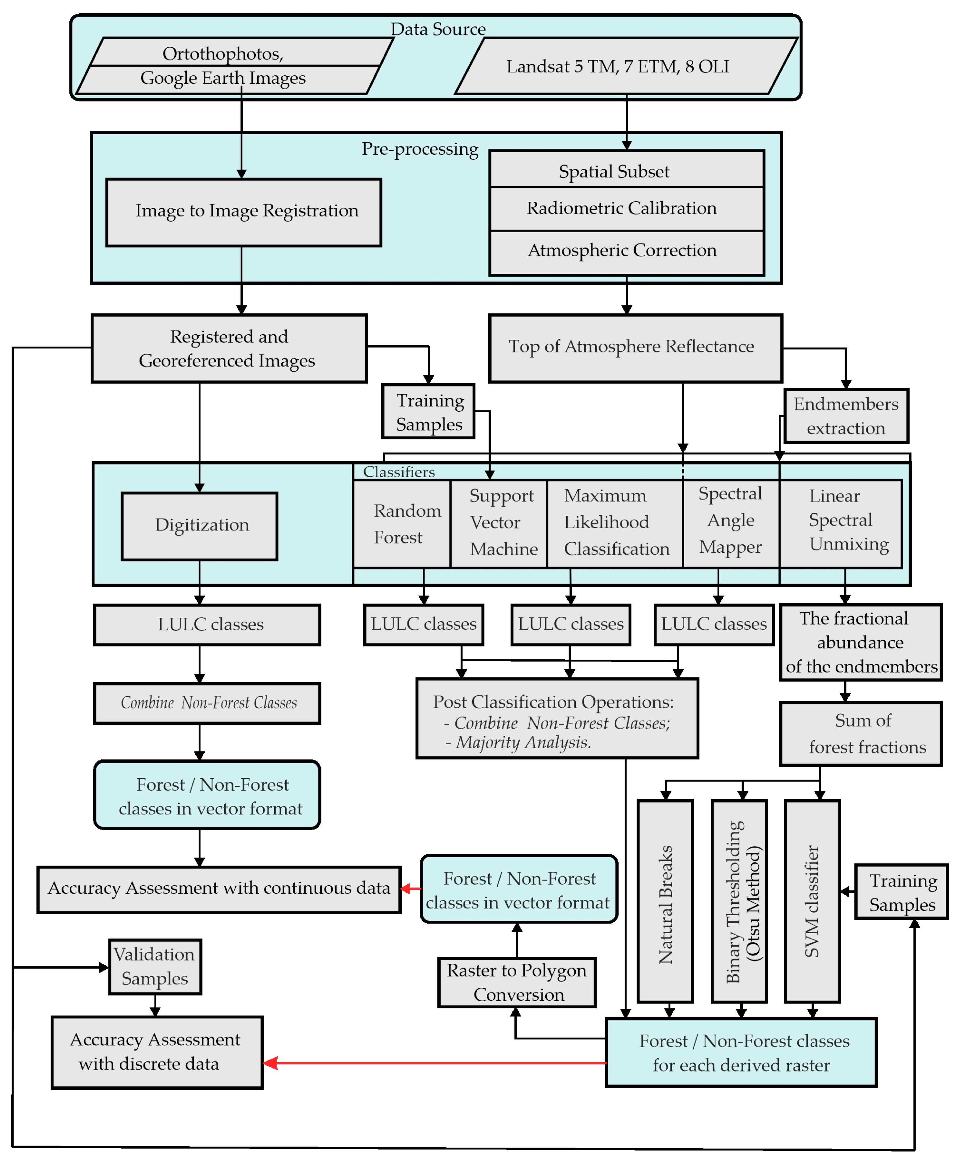
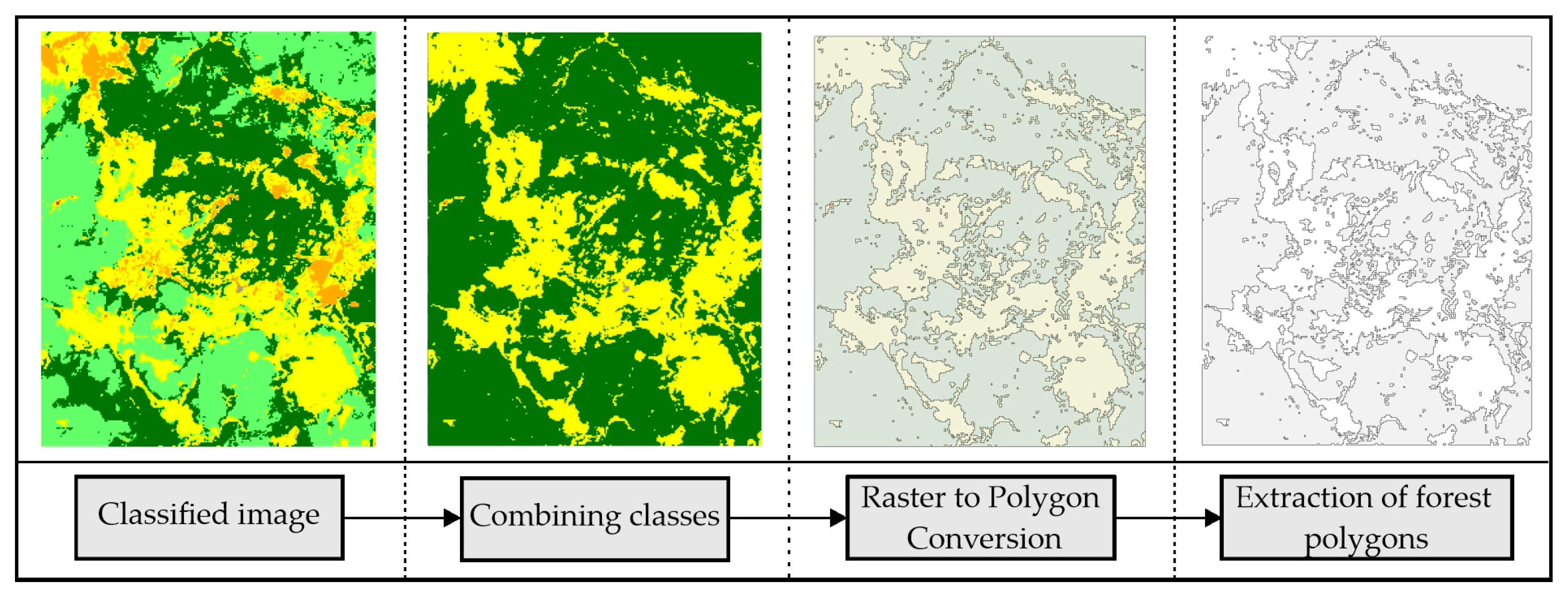
For this study, we used two types of data, which we will generically refer to as Data for GIS processing and Remote Sensing Data (Table 1). The selection of these data was based on several criteria, such as cloud cover and the period of the year with the most intense physiological activity of the forest, but the primary consideration was their temporal correspondence (year). We identified eight data sets covering a 17-year period.
The first type of data comprised orthophotos with a 0.5 m resolution from the National Agency for Cadastre and Land Registration (ANCPI) and Google Earth images (captured with the Google Earth Pro application) which were used for digitizing forest polygons. Prior to use, all Google Earth data underwent an image-to-image registration procedure [56] based on the orthophoto from 2012 with the highest location precision (20 cm). The scale at which they were taken from the application is 1: 2000. For 2011, the Google Earth image was supplemented in the southern part with the 2012 orthophoto.
The Remote Sensing Data used in this study were the multispectral images from Landsat 5 TM, 7 ETM, and 8 OLI obtained from the United States Geological Survey (USGS) [57] as Level 1 Products and geometrically calibrated by the satellite data providers. We mention that the Landsat 7 ETM scene does not have any data gaps, with it being prior to 31 May 2003, when the Scan Line Corrector (SLC) failed. All data underwent standard pre-processing operations in ENVI 5.3, including spatial subset, radiometric calibration for the FLAASH module, and atmospheric correction. Radiometric calibration for the FLAASH module involved the transfer of data from digital number (DN) format to radiation values with a scale factor of 0.1. For the conversion of radiation values into Top of Atmosphere Reflectance (ToA), we used the Fast Line-of-sight Atmospheric Analysis of Spectral Hypercubes (FLAASH) with a single scale factor of 1 for all bands, as well as the mid-Latitude Summer Atmospheric Model, Tropospheric Aerosol Model, and Kaufman-Tanre Aerosol Retrieval.
To reduce the shading effect on ToA and transition to Surface Reflectance (SR), we used the Cosine Correction Method [58] in SAGA GIS, with a Digital Elevation Model (DEM) with a 5 m resolution generated by ANCPI in the Laki2 project [59] from LiDAR data.

2.3. Methods

Figure 2 and Figure 3 summarize the workflow for the methods used in this study. To obtain the forested area from orthophotos and Google Earth images, which we refer to as Forest_GIS (FGIS) in this study, we vectorized in ArcGIS 8.1 the land cover/use classes (forest, pasture, bare rock, road, and built area) in the series of eight images used. Subsequently, we extracted the vectorial layers related to the forest using a specific tool (“Select”). We assumed a linear error of 1 m among the GIS data and 4 m between these and the ones from the satellite scenes, respectively. After the overlay operations, errors ranging from 16 ha to 18 ha resulted from the shifting to a unique system of data projection (WGS_1984_UTM_Zone_34N), in addition to handling errors.
For the extraction of forest cover from SR, we used four standard classifiers (SAM, MLC, SVM, RF) and LSU.
Linear Spectral Unmixing (LSU) and Spectral Angle Mapper (SAM) are physics-based methods that share a procedural approach to some extent. They both rely on the extraction of endmembers, which correspond to the spectral response of material components that make up the pixels in an image [60]. However, the mathematical models used for extracting information from these spectral signatures differ between the two methods. LSU is a standard technique for processing multispectral and hyperspectral scenes, developed by Adams et al. [61]. It allows for the extraction of material component fractions (abundances) at the pixel level, viewed as endmembers. The model assumes that the spectral signatures from each pixel level can be expressed as a linear combination of endmembers balanced by their abundance [62]. SAM is a classification method developed by Kruse et al. [63] that determines the spectral similarity between reference spectra (spectral signatures of components viewed as endmembers) and the spectral response at the pixel level. The model considers only the angular difference expressed in radians between two compared spectra, treated as vectors in a space with n dimensions (given by the number of spectral bands), rather than the length of the spectral vectors. As a result, it is expected to be less sensitive to alterations in lighting conditions [64,65].
For both methods, we used the same set of endmembers, one for each year, identified at the pixel level, and extracted the spectral signatures directly from the reflectance of the year in question using the Pixel Purity Index algorithm [66,67]. We combined this with a supervised assessment using orthophotos, Google Earth images, and fieldwork.
Each set of spectra in our study comprises two spectral signatures for the forest, two for the grassland, one for the road and built areas (due to resolution limitations), and sequentially, one for bare rock (not for all years). From 2009 onwards, we added another spectral signature for recently clear-cut land. Field observations showed that the two spectral signatures for the forest are primarily explained by the dominant species (coniferous forest and broad-leaved forest) and the different lighting/exposure of forest areas. For grassland, we distinguished between normal grassy surfaces and nearly degraded ones based on the continuity of the grassy vegetal cover.
In the scientific literature, there are several procedures for interpreting and analyzing fractions with forest vegetation or only with vegetation [68,69,70,71,72,73,74]. We selected two procedures based on image segmentation according to threshold values (NB and OM) and one that involves the use of a classifier (SVM).
In all three procedures, we worked with rasters resulting from the sum of fractions with forest vegetation from each LSU (for each year) using the Band Math tool in ENVI. Mathematically, this procedure is correct because if the LSU processing is done correctly, the overall sum of fractions at the pixel level cannot exceed 1 (the values are between 0 and 1 because we used the “unit sum constraint” conditioning).
NB, also known as Jenks Natural Breaks Method, is widely used in GIS software [75] and remote sensing studies [76,77,78]. We used NB to obtain an initial separation of rasters into two classes, after which we analyzed the threshold values (break values) and noticed a small degree of variation between 0.56–0.64 (with five out of seven values close to 0.6). To homogenize the procedure, we chose the threshold value of 0.6 to separate the two classes. In other words, pixels with a proportion of trees exceeding or equal to 60% were classified as forest. We reclassified each raster to transform it into an integer format and then into a vector layer from which we extracted the forest polygons forming FUNMIX_NB for the forthcoming analysis.
OM is a non-parametric and unsupervised method of automatic threshold selection for image segmentation [79], widely described in the literature [80,81] and commonly used in remote sensing [82,83,84]. We implemented it as Binary Thresholding in ArcGIS Pro [85] to separate forest/non-forest classes on rasters with added-up forest abundances.
The use of a classifier on LSU derivatives is a frequent procedure [66,69,86] for establishing LULC or resolving some problems of classification/ambiguity at the pixel level [87]. We chose SVM, and the details of this method are presented below. The forest polygons resulting from the conversion of new rasters derived through LSU with OM and LSU with SVM, respectively, form the vector layers called FUNMIX_OM and FUNMIX_SVM in this study.
Regarding the processing of rasters resulting from SAM, we performed two Post Classification operations on each of them: Combine Classes for compatibility and comparison with cu FGIS and Majority Analysis for spatial homogenization of the classes. Furthermore, we exported the SAM rasters in ArcGIS, converted them into vectorial formats, and extracted forest polygons, which we refer to as Forest_SAM (FSAM) in this study.
Support Vector Machine (SVM) and Random Forest (RF) are two supervised classification methods, non-parametric, from the Machine Learning family, requiring training samples acquired from the field or images with excellent resolution. Although similar in terms of entry data requirements, SVM and RF differ fundamentally in terms of the mathematical logic of class separation. SVM is based on the optimal margin method for separable data, identifying a hyper-plane that separates the data, and the kernel method for tracking them with a non-linear transformation to a higher dimensional space [88,89]. RF is based on plotting decision trees by using the Classification and Regression Trees Algorithm (CART), decision trees that make independent predictions by training on randomly extracted subsets from the entry data, and the final prediction is a result of combined individual predictions. [90,91]. SVM is based on the principle of statistical learning theory, conceptualized by Vapnik [92], and probably at present, alongside RF, is one of the most used methods of classification of multi and hyperspectral data [93,94] because it can be used with good results even when the territorial complexity is higher, and the information providing a consistent training data is lower. We used SVM with the Radial Basis Function kernel type, and for RF, we selected 150 decision trees, bearing in mind the actual recommendations [95].
Maximum Likelihood Classification (MLC) is a parametric classifier that uses the Bayesian Decision Rule to calculate the probability of an element being a member of each n class [96,97], and that requires, much like SVM and RF, training samples as entry data, alongside multispectral images.
The training data set for each year was extracted using orthophotos and Google Earth images (Table 2), representing approximately 27% of the 72,600 pixels covering the study area. The same pixels were used for SVM, RF, and MLC for comparison purposes, and the LULC classes were kept the same as for SAM and LSU, except for the clear-cut surfaces, which were integrated with pastures.
The SVM, RF, and MLC rasters underwent the same post-classification operations as those from SAM, and the resulting vector layers with forest were named Forest_SVM (FSVM), Forest_RF (FRF) and Forest_MLC (FMLC), respectively. We mention that all the final data used in the comparative analysis for forested areas are also in vector format. Extraction and overlay vectorial (intersect, symmetrical difference) techniques were then applied in order to obtain the necessary data for the comparative analysis and evaluation for the accuracy of the results.

2.4. Accuracy Assessment

In this study, we conducted an assessment of both thematic accuracy [98] and spatial accuracy [99] in line with our intended objectives.
For the assessment of thematic accuracy, we worked with two versions of Producer’s Accuracy and User’s Accuracy, which we refer to as PA1/UA1 and PA2/UA2, respectively, to avoid confusion. Both versions have the same significance: Producer’s Accuracy indicates the probability of a reference sample being correctly classified, and User’s Accuracy indicates the probability that a sample classified represents that category on the ground [100]. The differences arise from the type of data used for validation samples. We used training samples at the pixel level for PA1/UA1, with a Stratified Random sampling scheme and 200 samples on each raster in a forest/non-forest format, in accordance with current recommendations [101,102].
We introduced PA2/UA2, which was developed by Zhan et al. [103] for assessing the accuracy of geospatial objects, to match our aim of conducting comparative assessments between FGIS and FUNMIX_NB, FUNMIX_OM, FUNMIX_SVM, FSVM, FRF, and FMLC.
PA 2 = C R R
UA 2 = C R C
where C represents the area of the classified object (in our case, the forest area from classification), R represents the area of the reference object (in our study, the forest area from digitization—FGIS), and C R represents the area of the intersection between C and R.
For spatial accuracy assessment, we used Overall Quality (OQ) [99,103]:
OQ = C R ¬ C R + C ¬ R + C R  
where ¬ C R represents the area of R that is not covered by C, and C ¬ R represents the area of C that is not covered by R.

3. Results

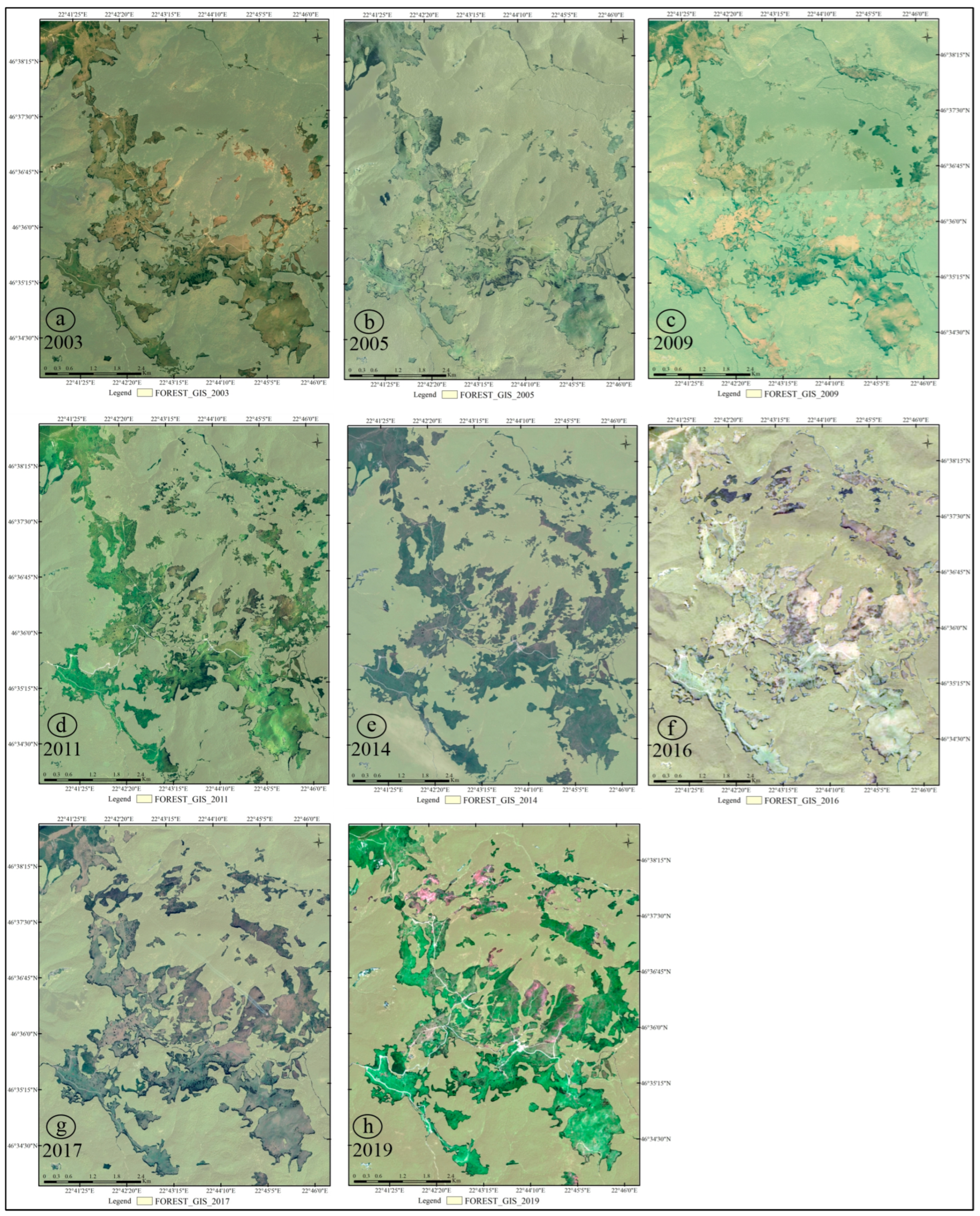
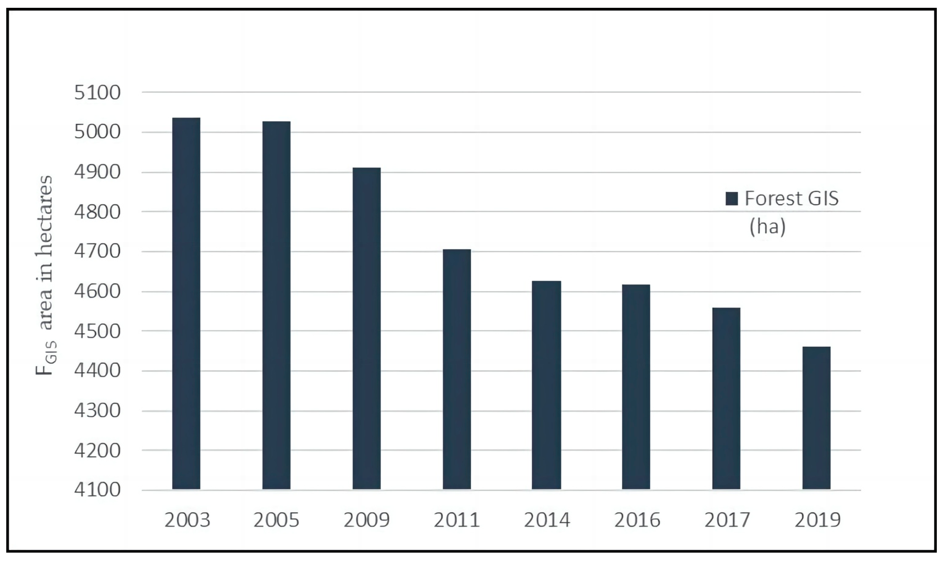
3.1. Monitoring Forest Area with GIS Data

We analyzed the dynamics of forest cover in the study area using data obtained through digitization (FGIS). These data are presented spatially in Figure 4 and quantitatively in Table 3, indicating a decrease in the forest area of 577 hectares from 2003 to 2019, resulting in an average rate of decrease of 33.9 hectares per year for the forest area. In terms of percentage, we observed a reduction in the degree of forestation from 77% to approximately 68% for the analyzed territory over just 17 years.
Two aspects need to be addressed here. Firstly, the value of 577 hectares should be understood as a net quantitative loss, as there are areas where the forest has extended into the territory due to natural regeneration during the 17 years analyzed. Symmetrical Difference operations performed on the vector layers reveal a spatial increase of 164 hectares and a decrease of 741 hectares.
Secondly, regarding the average rate, there were no significant negative alterations (decrease) or positive ones between 2003 and 2005, and the time frame was too short for any increase phenomenon to be (noticeable) considerable. From 2005 to 2009, there was a moderate decrease in the forest by 117 hectares, with an average decrease rate of 23.4 hectares per year for five years. However, from 2009 to 2011, there was a dramatic decrease of 205.25 hectares, with an average rate for the three years of 68.41 hectares per year, as shown in the diagram in Figure 5.
The rate of decrease in forest cover during the last three years (2017–2019) is consistent with the average rate observed over the 17 years analyzed.

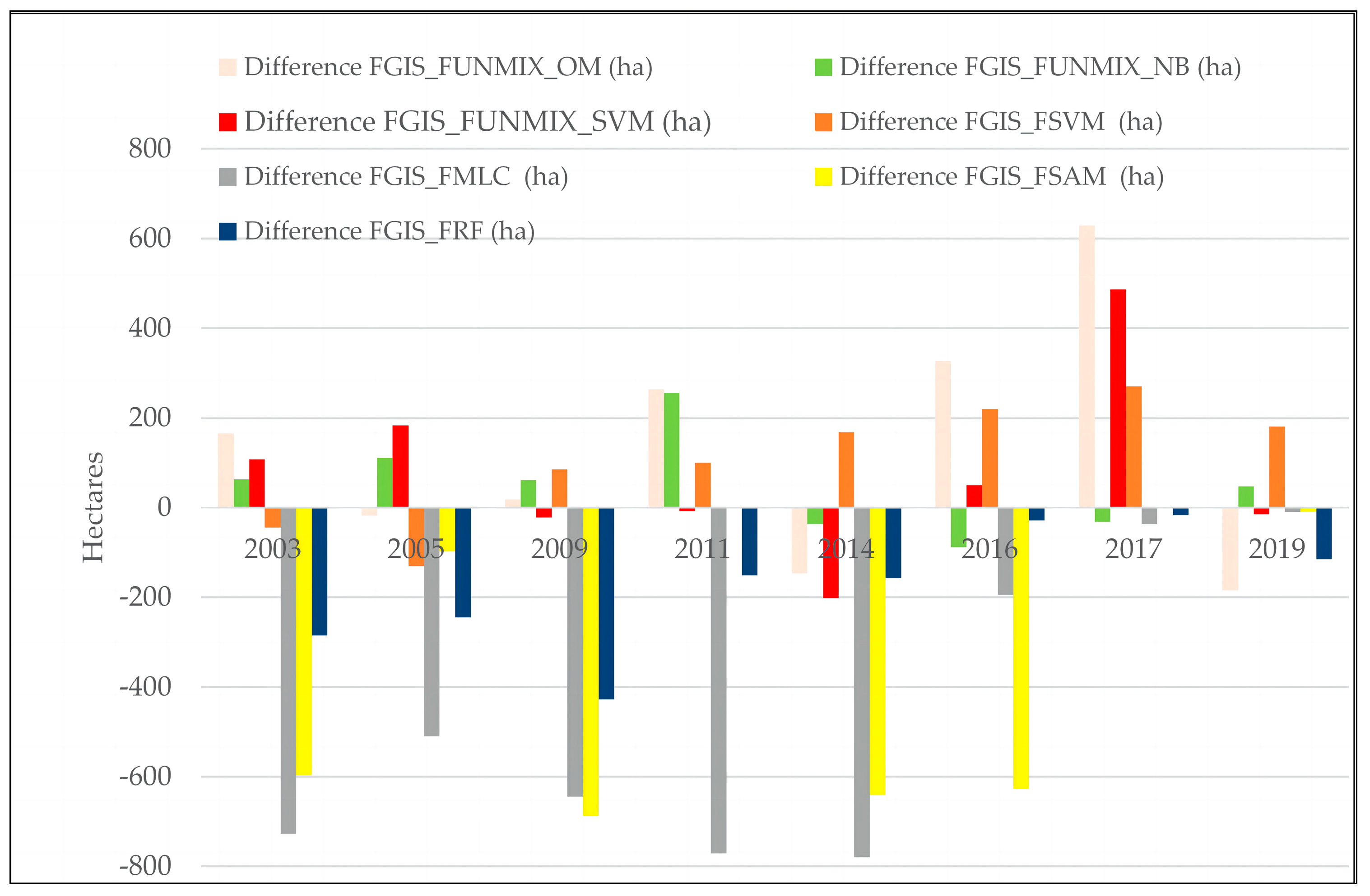
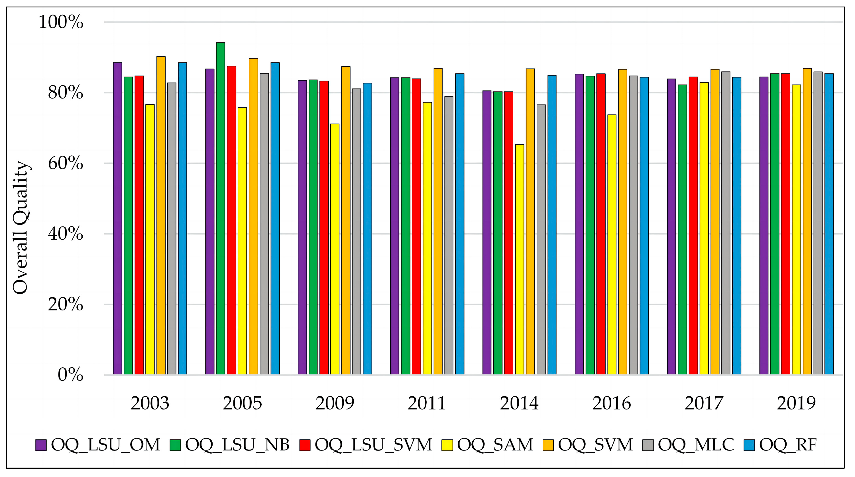
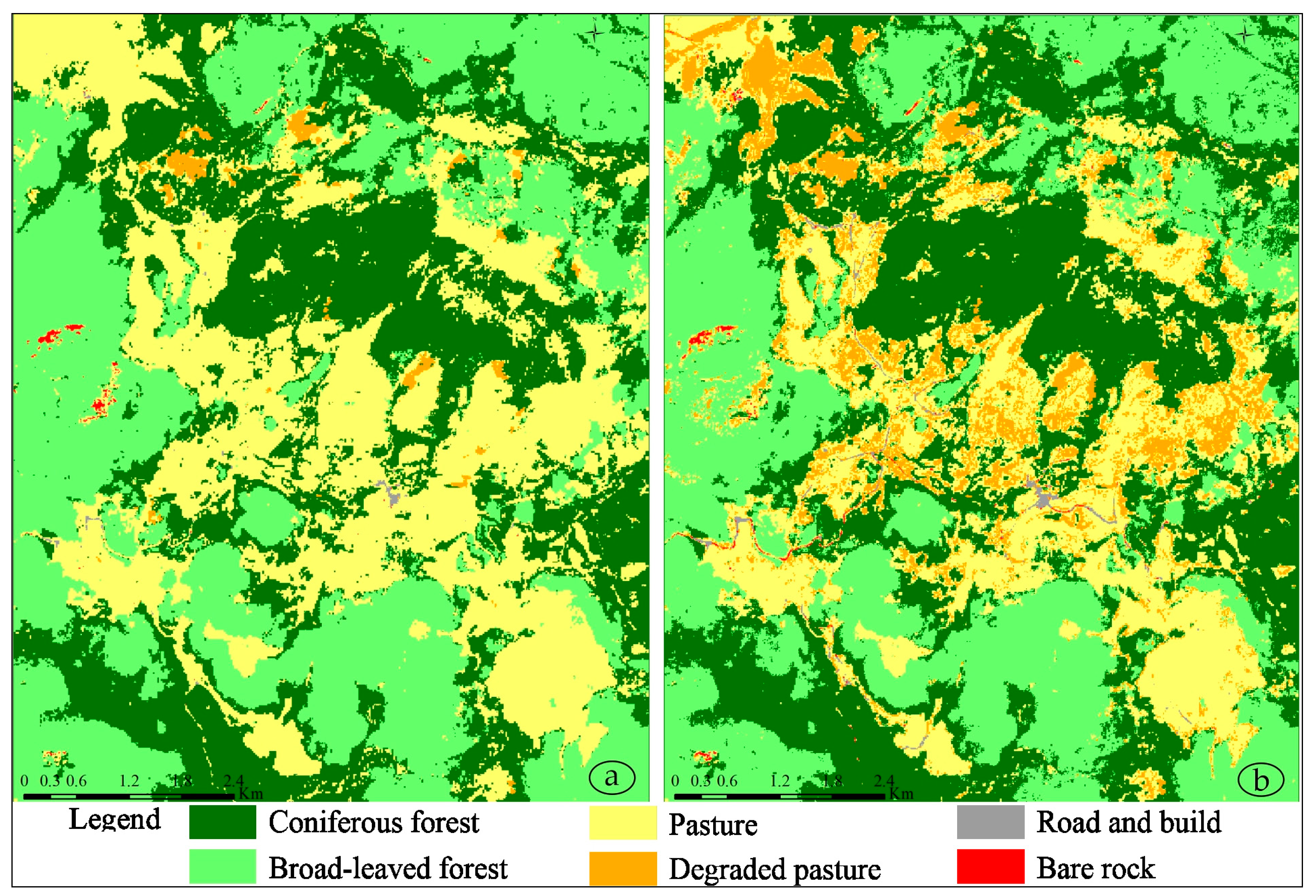
3.2. Comparative Analysis

The comparative analysis of the methods used, from the perspective of the results achieved (FGIS, FUNMIX_NB, FUNMIX_OM, FUNMIX_SVM, FSAM, FSVM, FMLC, FRF), focuses on three key aspects: the quantitative correspondence of absolute values (i.e., the value in hectares obtained from each layer) of forest cover, the thematic accuracy (i.e., how well the forest area is extracted), and the spatial accuracy of classifications.
To assess the quantitative correspondence of absolute values, we analyzed the forest areas of FUNMIX_NB, FUNMIX_OM, FUNMIX_SVM, FSAM, FSVM, FMLC, and FRF (as shown in Table 4) in relation to disparities compared to FGIS (as shown in Table 5), which were categorized as positive (overestimation) or negative (underestimation) and summed up to obtain terms for comparison. This type of analysis is known as “non-site-specific analysis” in the literature [101].
As shown in Figure 6, the smallest deviations were observed for FUNMIX_NB and FUNMIX_SVM, followed by FSVM, while the largest deviations were observed for FMLC and FSAM. For FUNMIX_NB, there were five situations of overestimation (one of which was insignificant at +47 hectares) and three years of negative deviations (two of which were significant). The average value of total deviations (694.11 hectares) for the eight years for FUNMIX_NB was 86.76 hectares. For all the forest area forms derived from LSU, there was a prevalence of positive deviations, with an additional 1406 hectares for FUNMIX_OM.
In the case of FSVM, there was a clear tendency of overestimation, with positive deviations observed in six out of the eight years for which we have data. The average value of total deviations (1200.29 hectares) for the eight years for FSVM was 150 hectares. For FRF, the deviations are only negative, with an average of 170 hectares.
These data provided a partial comparison of the values obtained through the methods used in this study, as they do not provide information on the quality of classifications or the spatial correspondence of forest areas.
To assess thematic accuracy, we used two versions of Producer’s Accuracy and User’s Accuracy (PA/UA), which offer multiple possibilities for comparison. These include comparative assessments of thematic accuracy for the methods used, indirect assessments (through comparison) of accuracy for FGIS, and comparative analyses between the two versions of calculation for PA and UA. Table 6 lists the values for PA1 and PA2.
As individual values, PA ranges from 99% (PA1 for LSU_SVM in 2019) to 73% (PA2 for SAM in 2014), with an average of 90.8%. Only five PA values out of 112 are in the acceptable accuracy class (70–79%) [104], while the others belong to the high accuracy class (80–89%, 25 values) and very high accuracy class (over 90%, 82 values). Comparing PA1 and PA2, the difference between the pair values is generally not significant, with 80% of cases ranging between 1–3% in favor of PA1 (with only 11 situations out of 56 obtaining higher scores for PA2). LSU_OM and LSU_SVM (95%) have the best score for PA1 as the mean value for the entire time frame, while SVM has the best result (94%) for PA2. SVM also stands out for its consistently high values on both series of results (94% for PA1 and PA2).
Statistics for UA (Table 7) show a net prevalence of values belonging to the very high accuracy class and high accuracy class, with two maximum values of 99% obtained by MLC for the UA1 version and a minimum of 84% for SAM in the UA2 version. Comparing UA1 and UA2, the proportion of the difference between the pair values that range between 1–3% is only 69%, with UA2 exceeding UA1 in only three cases out of 56. The MLC and RF classifiers have the best scores for UA1 and UA2, followed by SVM and LSU_NB based on mean values for both UA1 and UA2.
Overall Quality (OQ) for single-class assessment [99,103] quantifies spatial accuracy by considering both the degree of overlap and non-overlap (as shown in Equation (3)).
The results for OQ, presented numerically in Table 8 and graphically in Figure 7, exceed the critical value of 50%, which is the lower threshold for validation and use in assessing spatial accuracy [99]. The best score for each value separately was recorded by LSU_NB in 2005 (94%), while the lowest OQ was recorded by SAM in 2014 (65%). Statistically, the range of 80–90% (45 values out of 56, or 80% of the results) has the highest frequency in the series of results for OQ.
Based on the average series of values, SVM has the best spatial accuracy with an 88% OQ, followed by RF with 86%. If we exclude SAM, which has a lower OQ with an average of 76%, all the other methods consistently obtained scores above 80%.
The main problem that this study aims to address is identifying the best method for extracting a forest area that corresponds to the actual situation on site. Table 9 provides a ranking of the methods used based on the results assessed through performance metrics. By using a simple arithmetic average of values without weighting criteria importance (equivalent to performance indices), we can obtain an average ranking position that translates easily into an Overall Ranking (OR) for the methods used. Comparing the positions in this OR with those in OQ, it is noticeable that the situation is identical, which further emphasizes the importance of OQ as a measure of spatial accuracy.
SVM stands out not only for its first two positions in PA2 and OQ but also for its consistently high positions in all the accuracy assessments presented. In contrast, SAM records the lowest positions in the hierarchies listed in Table 9.
It is worth noting that although the differences between the scores obtained by the methods used are small, only a 1% difference actually corresponds to a difference of 40–50 hectares (depending on the year). RF occupies the second position, with the best results for UA1 and two second positions at UA2 and OQ. Much like SVM, it stands out for consistently high results regarding OQ. LSU_NB closely follows RF (with a difference of only 0.6 in the average ranking positions) but does not register any first place for the performance indicators used. Although LSU_SVM has the best score for PA1 (along with LSU_OM), it is outperformed by SVM and LSU_NB for other performance measures. LSU_OM has very good results for PA, but it overestimates the forest area, which explains its fourth and fifth-place rankings in OQ and UA2, respectively. It is important to note that none of the LSU combinations were able to accurately assess the situation in 2014, which had a cloud cover of 2.93%, not even when combined with a non-parametric method like SVM. The effects of the masked pixels in 2014 are best seen in the scores for PA (Table 6) and OQ (Table 8). Only SVM and RF maintained their high percentage for all performance indicators in that year, which can be explained by the way these classifiers work (as discussed in Section 2.3). There is no sensible explanation for the behavior of LSU_SVM in 2014. However, both LSU_SVM and SVM were able to identify the sudden decrease in forest area between 2009 and 2011, while other versions of LSU and SAM were not able to capture it. The explanation for this can be found in the metadata of the images used in the study. The multispectral Landsat 5 image used was from July 2011, while the Google Earth image was from October 2011, which suggests that the land clearing may not have been captured by the Landsat image. Unfortunately, the study does not have data to precisely show the period of logging.
One interesting finding in this study is the rather unusual situation observed with MLC, which occupies the first position at UA, regardless of the version, with very high scores, but weaker results at PA, OQ, and QC. This suggests that MLC is very effective at classifying pixels identified as part of a particular class (in this case, the forest), but it struggles with omission errors.
An important aspect of any comparative study regards highlighting the behavior of the used classifiers when the entry data are changing. Accordingly, a small experiment was conducted using a Sentinel 2 MSI-Level 2A (SR) satellite scene from July 2019, obtained from the Copernicus Scientific Hub [105]. Four spectral bands with a resolution of 10 m (Blue, Red, Green, and Near-Infrared) and six with a resolution of 20 m (Red-edge 1, Red-edge 2, Red-edge, NIR narrow, and two SWIR bands) were extracted from the scene. The bands with a resolution of 20 m were resampled to 10 m, and then all 10 bands were combined to create two multi-band files: one having only Sentinel bands, and the other, in which were combined the spectral bands from Landsat 8 image (2019, resampled to 10 m) used in this study with the three red-edge bands dedicated to vegetation in Sentinel. These files were then used with the SVM and RF classifiers, which offered the best results in this study. The resulting classified images (those presented in Figure 8 are derived from the first multi-band file—Sentinel 10 m) were processed and evaluated for accuracy according to the methodology used. If we compare the accuracy indices values obtained on these 2 data sets (Table 10) with the performance indices average values registered by SVM and RF on the classified images from Landsat scenes, we observe that RF obtains scores up to 6% higher than the average indices (at PA1), while SVM has moderate increases or stagnates. This aspect would indicate a higher potential for RF, even if it obtains second place in our hierarchy.

4. Discussion

One of the guidelines of this study follows the use of some performance indices to express the spatial accuracy of the results obtained. If we had not used performance measures for assessing spatial accuracy and instead relied solely on continuous data for thematic accuracy, such as removing PA2, UA2, and OQ, then RF would occupy fourth position in terms of performance, and LSU_OM would be in first position, along with SVM, followed by LSU_SVM. However, if we had used Overall Accuracy (OA), then RF would have been considered the best performer (with a mean value of 93% for OA), and SVM would only occupy the third position. We did not use OA in this study because previous research [99,103,105,106] has shown that OA takes into account those pixels that are not part of the class of concern (in this case, the forest). Therefore, for a single-class assessment, it is advisable to use PA and UA.
Regarding the occurrence and spatial distribution of errors that appear in the classification procedures carried out, it can be observed that irrespective of their type (omission and commission) and the classification method used (which can affect the extent of errors), as illustrated in Figure 9, errors are predominantly localized in marginal forest strips that transition to pastures, recently deforested areas, and regions with sparse arboreal vegetation.
As a secondary aspect of our analysis, we address the issue of interpreting LULC classes from the CORINE 2018 database [55], specifically the Transitional woodland-shrub class (code 324). Some polygons within this class represent recent clear-cut areas where the forest has completely disappeared, at least in the territory we studied (Figure 10). Although we did not incorporate the CORINE Land Cover data in our comparative analysis due to the mismatch between the scales (1:100,000) used in the dataset, which covers almost a continental-size territory and cannot represent polygons under 25 km2 [107], and the finer resolution (0.5 m) of our digitized data, it is crucial to highlight that for adjacent years, the differences between the CLC and FGIS datasets are noteworthy. For instance, the differences in CLC and FGIS datasets for forest cover in 2000 and 2006 are negligible (175 ha underestimation in 2000 and 40 ha overestimation in 2006). However, for CLC 2016 and 2018, compared to FGIS 2016 and 2017, the differences are more significant (231 ha overestimation for 2016 and 326 ha overestimation for 2018, both values with a positive sign), despite the superior quality of satellite data (Landsat 8 OLI and Sentinel 2) used by CLC. The discrepancies in our study area can be attributed to the interpretation of CLC classes and the fragmentation of areas with dense forest.
Upon comparing our results with those obtained from high-resolution data sets, Dominant Leaf Type and Forest Type, available online at land.copernicus.eu [108], we observed even greater differences, particularly in overestimating the forest extent for the latter. The data indicated that the forest extent was 5290.24 ha in 2012 and 4953.7 ha in 2018. Additionally, considerable discrepancies were found when comparing our results with the sets of global data Forest extent—2000 and Forest extent—2020 [37], produced by the GLAD Landsat Analysis Ready Data team [36], which are also accessible online [109]. According to our processed data for Padiș, the forest extent was 5706 ha in 2000 and 5407 ha in 2020.
We wish to clarify the causes of the significant decrease in forest area in Padiș. Based on our research and observations, we assert that these causes are multifaceted. Natural factors, such as severe storms [110,111,112], causing windthrows (the latest one occurred on 17 September 2017), as mentioned in the PNA environmental reports [113,114,115,116,117,118], and pests, such as the European spruce bark beetle (Ips typographus) [119,120], have contributed to this decline. Furthermore, the damaged wood provides an opportunity for exploitation, even in protected areas, as allowed by Romanian laws. However, the amount of wood harvested exceeds the amount naturally damaged, resulting in legal loggings being transformed into illegal ones. Such illegal activities are well documented in the literature [121,122].
How do our findings fit into the context of similar studies that focus on the comparative evaluation of the methods employed? Taking into account the studies cited in Section 1, alongside additional ones, we can place this study in the “group” that obtained better results for SVM and RF. This assertion is because the accuracy scores of important classifiers in other studies vary [94]. However, it can be challenging to make quantitative comparisons between the results due to the different performance metrics used [123,124,125,126].
For SVM, we mention several studies with better results, including Pal and Mather [127], Rokni Deilmai et al. [128], Abe et al. [66], Maxwell et al. [129], Thanh Noi and Kappas [47], Hasan et al. [130], Nguyen et al. [49], Zagajewski et al. [29], and Dabija et al. [51]. The latter [51] obtained the best scores for SVM with Radial Basis Function compared to RF for the CLC classes. For classes 311 (deciduous forests) and 313 (mixed forests), the overall accuracy ranges between 63–98% and 75–83%, respectively. For class 324 (Transitional woodland-shrub), the overall accuracy ranges from a minimum of 56% to a maximum of 82%.
Among the comparative studies in which RF has the best results or obtains similar results to SVM, we mention those carried out by Adugna et al. [48], Rodriguez-Galiano et al. [131], Christovam et al. [132], Tomala et al. [133], Bayrakdar et al. [134], and Avci et al. [135]. The scores obtained for RF by Forkuor et al. [46] are also remarkable, which surpass 90% OA, even if they are slightly outrun by SGB.
For the Unmixing approach, Lu et al. [20] used LSU with the threshold method to classify vegetation from the Amazon basin and compared the results with MLC, resulting in an extra 7.4% OA for LSU. Taureau et al. [73] used LSU and NDVI in a comparative study of the mangrove forest canopy obtained from hemispherical photographs and found an excellent correlation for LSU (R2—0.95). Ruggeri et al. [50] found the best results for the LSU-OBIA combination, with a User’s Accuracy of 88%. However, Medina Machín et al. [86] obtained weaker results for the LSU with SVM (81.4% OA) version in a study for the classification of vegetation in a coastal-dune ecosystem, despite using various combinations of spectral bands, vegetation indices, textural parameters, and fractional abundances from LSU.
Regarding our results from MLC and SAM, they align with the line of research that employs these methods. Sohn et al. [136] used a version of SAM in a study on deforestation and forest recovery stages in Yucatan, which yielded results exceeding 70% UA. Shafri et al. [44] obtained 85.56% OA for MLC and only 48.83% OA for SAM. Li et al. [137] evaluated various spectral combinations from Landsat TM, vegetation indices, and classification methods, including MLC, concluding that MLC and OBIA offered the best results.

5. Conclusions

This study analyzes changes in forest cover in a protected area by integrating remote sensing processing results with GIS to assess accuracy, which is the most sensitive aspect of this approach. The complementary nature of remote sensing and GIS provides real support for monitoring forest areas in protected areas, given the easy access to satellite data, continuous method improvements, and minimal financial costs and time resources.
To ensure the best methods of work and quality assessment, it is crucial to select appropriate measures. Therefore, we advocate for the widespread use of spatial accuracy indices, particularly in situations where the use of performance metrics alone at the pixel level may lead to incorrect interpretations, as we hypothetically presented.
Regarding our study area, which is integrated into PNA, no other studies monitor territorial forest cover changes, regardless of the CLC database. CLC is only tested for thematic accuracy [107]. Our study reveals that the forest area decreased continuously in two time sequences (2005–2014, 2016–2019) within the analyzed time frame of 17 years (2003–2019), resulting in a net loss of 577 ha, which equates to a 9% decrease in forestation.
Of all the methods used, SVM and RF estimate this situation the best. SVM stands out by a consistent behavior, slightly better than RF, as demonstrated by the obtained performance scores and by the fact that it highlights the reduction in forested areas more effectively. RF responds better to changes in entry data, indicating that its performance can be improved.

Author Contributions

Conceptualization, L.B. and D.C.I.; methodology, L.B., J.A.W., I.R. and K.Z.; software, L.B., J.A.W., I.R. and K.Z.; validation, J.A.W., I.R. and K.Z.; formal analysis, J.A.W., I.R. and K.Z.; investigation, J.A.W., I.R. and K.Z.; resources, K.Z. and L.D.D.; data curation, L.B. and D.C.I.; writing—original draft preparation, L.B., D.C.I. and K.Z.; writing—review and editing, L.B., D.C.I. and K.Z.; visualization, D.C.I.; supervision, D.C.I., K.Z. and L.D.D.; project administration, D.C.I., K.Z. and L.D.D.; funding acquisition, D.C.I., K.Z. and L.D.D. All authors have read and agreed to the published version of the manuscript.

Funding

The research has been funded with the support of the University of Oradea. The research undertaken was made possible by the equal scientific involvement of all the authors concerned.

Data Availability Statement

Data developed in this study will be made available on request to the corresponding authors.

Acknowledgments

This research was supported by the Hungarian University of Agriculture and Life Sciences and the Doctoral School of Economic and Regional Sciences (MATE), Hungary.

Conflicts of Interest

The authors declare no conflict of interest.

References

  1. Bonnesoeur, V.; Locatelli, B.; Guariguata, M.R.; Ochoa-Tocachi, B.F.; Vanacker, V.; Mao, Z.; Stokes, A.; Mathez-Stiefel, S.-L. Impacts of forests and forestation on hydrological services in the Andes: A systematic review. For. Ecol. Manag. 2019, 433, 569–584. [Google Scholar] [CrossRef] [Green Version]
  2. Chen, H.; Zeng, Z.; Wu, J.; Peng, L.; Lakshmi, V.; Yang, H.; Liu, J. Large Uncertainty on Forest Area Change in the Early 21st Century among Widely Used Global Land Cover Datasets. Remote Sens. 2020, 12, 3502. [Google Scholar] [CrossRef]
  3. Wang, W.J.; Ma, S.; He, H.S.; Liu, Z.; Thompson, F.R., III; Jin, W.; Wu, Z.F.; Spetich, M.A.; Wang, L.; Xue, S.; et al. Effects of rising atmospheric CO2, climate change, and nitrogen deposition on aboveground net primary production in a temperate forest. Environ. Res. Lett. 2019, 14, 104005. [Google Scholar] [CrossRef]
  4. Duveneck, M.J.; Thompson, J.R. Climate change imposes phenological trade-offs on forest net primary productivity. J. Geophys. Res. Biogeosci. 2017, 122, 2298–2313. [Google Scholar] [CrossRef]
  5. Peters, E.B.; Wythers, K.R.; Zhang, S.; Bradford, J.B.; Reich, P.B. Potential climate change impacts on temperate forest ecosystem processes. Can. J. For. Res. 2013, 43, 939–950. [Google Scholar] [CrossRef]
  6. IPCC. Climate Change 2022: Impacts, Adaptation, and Vulnerability. Contribution of Working Group II to the Sixth Assessment Report of the Intergovernmental Panel on Climate Change; Pörtner, H.-O., Roberts, D.C., Tignor, M., Poloczanska, E.S., Mintenbeck, K., Alegría, A., Craig, M., Langsdorf, S., Löschke, S., Möller, V., et al., Eds.; Cambridge University Press: Cambridge, UK; New York, NY, USA, 2022; p. 3056. Available online: https://www.ipcc.ch/report/ar6/wg2/ (accessed on 11 May 2023).
  7. Keenan, T.F.; Gray, J.; Friedl, M.A.; Toomey, M.; Bohrer, G.; Hollinger, D.Y.; Munger, J.W.; O’keefe, J.; Schmid, H.P.; Wing, I.S.; et al. Net carbon uptake has increased through warming-induced changes in temperate forest phenology. Nat. Clim. Chang. 2014, 4, 598–604. [Google Scholar] [CrossRef]
  8. Chivulescu, S.; García-Duro, J.; Pitar, D.; Leca, Ș.; Badea, O. Past and Future of Temperate Forests State under Climate Change Effects in the Romanian Southern Carpathians. Forests 2021, 12, 885. [Google Scholar] [CrossRef]
  9. Mihai, G.; Alexandru, A.-M.; Nita, I.-A.; Birsan, M.-V. Climate Change in the Provenance Regions of Romania over the Last 70 Years: Implications for Forest Management. Forests 2022, 13, 1203. [Google Scholar] [CrossRef]
  10. Romeiro, J.M.N.; Eid, T.; Antón-Fernández, C.; Kangas, A.; Trømborg, E. Natural disturbances risks in European Boreal and Temperate forests and their links to climate change—A review of modelling approaches. For. Ecol. Manag. 2022, 509, 120071. [Google Scholar] [CrossRef]
  11. Senf, C.; Seidl, R. Mapping the forest disturbance regimes of Europe. Nat. Sustain. 2020, 4, 63–70. [Google Scholar] [CrossRef]
  12. Forest Europe. State of Europe’s Forests 2020. Available online: https://foresteurope.org/state-europes-forests-2020/ (accessed on 5 April 2022).
  13. Forzieri, G.; Girardello, M.; Ceccherini, G.; Spinoni, J.; Feyen, L.; Hartmann, H.; Beck, P.S.A.; Camps-Valls, G.; Chirici, G.; Mauri, A.; et al. Emergent vulnerability to climate-driven disturbances in European forests. Nat. Commun. 2021, 12, 1081. [Google Scholar] [CrossRef] [PubMed]
  14. Wang, K.; Franklin, S.E.; Guo, X.; Cattet, M. Remote Sensing of Ecology, Biodiversity and Conservation: A Review from the Perspective of Remote Sensing Specialists. Sensors 2010, 10, 9647–9667. [Google Scholar] [CrossRef] [PubMed]
  15. Kumar, D. Monitoring Forest Cover Changes Using Remote Sensing and GIS: A Global Prospective. Res. J. Environ. Sci. 2011, 5, 105–123. [Google Scholar] [CrossRef] [Green Version]
  16. Thompson, I.D.; Guariguata, M.R.; Okabe, K.; Bahamondez, C.; Nasi, R.; Heymell, V.; Sabogal, C. An Operational Framework for Defining and Monitoring Forest Degradation. Ecol. Soc. 2013, 18, 20. [Google Scholar] [CrossRef]
  17. Grecchi, R.C.; Beuchle, R.; Shimabukuro, Y.E.; Aragão, L.E.; Arai, E.; Simonetti, D.; Achard, F. An integrated remote sensing and GIS approach for monitoring areas affected by selective logging: A case study in northern Mato Grosso, Brazilian Amazon. Int. J. Appl. Earth Obs. Geoinf. 2017, 61, 70–80. [Google Scholar] [CrossRef]
  18. Mitchell, A.L.; Rosenqvist, A.; Mora, B. Current remote sensing approaches to monitoring forest degradation in support of countries measurement, reporting and verification (MRV) systems for REDD+. Carbon Balance Manag. 2017, 12, 9. [Google Scholar] [CrossRef] [Green Version]
  19. Adams, J.B.; Sabol, D.E.; Kapos, V.; Almeida Filho, R.; Roberts, D.A.; Smith, M.O.; Gillespie, A.R. Classification of multispectral images based on fractions of endmembers: Application to land-cover change in the Brazilian Amazon. Remote Sens. Environ. 1995, 52, 137–154. [Google Scholar] [CrossRef]
  20. Lu, D.; Batistella, M.; Morán, E.; Mausel, P. Application of spectral mixture analysis to Amazonian land-use and land-cover classification. Int. J. Remote Sens. 2004, 25, 5345–5358. [Google Scholar] [CrossRef]
  21. Johnson, B.; Tateishi, R.; Kobayashi, T. Remote Sensing of Fractional Green Vegetation Cover Using Spatially-Interpolated Endmembers. Remote Sens. 2012, 4, 2619–2634. [Google Scholar] [CrossRef] [Green Version]
  22. Liu, G.; Li, L.; Gong, H.; Jin, Q.; Li, X.; Song, R.; Chen, Y.; He, C.; Huang, Y.; Yao, Y. Multisource Remote Sensing Imagery Fusion Scheme Based on Bidimensional Empirical Mode Decomposition (BEMD) and Its Application to the Extraction of Bamboo Forest. Remote Sens. 2016, 9, 19. [Google Scholar] [CrossRef] [Green Version]
  23. Linhui, L.; Weipeng, J.; Huihui, W. Extracting the Forest Type from Remote Sensing Images by Random Forest. IEEE Sensors J. 2020, 21, 17447–17454. [Google Scholar] [CrossRef]
  24. Vohland, M.; Stoffels, J.; Hau, C.; Schüler, G. Remote sensing techniques for forest parameter assessment: Multispectral classification and linear spectral mixture analysis. Silva Fenn. 2007, 41, 471. [Google Scholar] [CrossRef] [Green Version]
  25. Heumann, B.W. An Object-Based Classification of Mangroves Using a Hybrid Decision Tree—Support Vector Machine Approach. Remote Sens. 2011, 3, 2440–2460. [Google Scholar] [CrossRef] [Green Version]
  26. Gudex-Cross, D.; Pontius, J.; Adams, A. Enhanced forest cover mapping using spectral unmixing and object-based classification of multi-temporal Landsat imagery. Remote Sens. Environ. 2017, 196, 193–204. [Google Scholar] [CrossRef]
  27. Raczko, E.; Zagajewski, B. Comparison of support vector machine, random forest and neural network classifiers for tree species classification on airborne hyperspectral APEX images. Eur. J. Remote Sens. 2017, 50, 144–154. [Google Scholar] [CrossRef] [Green Version]
  28. Liu, Y.; Gong, W.; Hu, X.; Gong, J. Forest Type Identification with Random Forest Using Sentinel-1A, Sentinel-2A, Multi-Temporal Landsat-8 and DEM Data. Remote Sens. 2018, 10, 946. [Google Scholar] [CrossRef] [Green Version]
  29. Zagajewski, B.; Kluczek, M.; Raczko, E.; Njegovec, A.; Dabija, A.; Kycko, M. Comparison of Random Forest, Support Vector Machines, and Neural Networks for Post-Disaster Forest Species Mapping of the Krkonoše/Karkonosze Transboundary Biosphere Reserve. Remote Sens. 2021, 13, 2581. [Google Scholar] [CrossRef]
  30. Asner, G.P.; Broadbent, E.N.; Oliveira, P.J.C.; Keller, M.; Knapp, D.E.; Silva, J.N.M. Condition and fate of logged forests in the Brazilian Amazon. Proc. Natl. Acad. Sci. USA 2006, 103, 12947–12950. [Google Scholar] [CrossRef] [Green Version]
  31. Hansen, M.C.; Stehman, S.V.; Potapov, P.V.; Loveland, T.R.; Townshend, J.R.G.; DeFries, R.S.; Pittman, K.W.; Arunarwati, B.; Stolle, F.; Steininger, M.K.; et al. Humid tropical forest clearing from 2000 to 2005 quantified by using multitemporal and multiresolution remotely sensed data. Proc. Natl. Acad. Sci. USA 2008, 105, 9439–9444. [Google Scholar] [CrossRef] [Green Version]
  32. Townshend, J.R.; Masek, J.G.; Huang, C.; Vermote, E.F.; Gao, F.; Channan, S.; Sexton, J.O.; Feng, M.; Narasimhan, R.; Kim, D.; et al. Global characterization and monitoring of forest cover using Landsat data: Opportunities and challenges. Int. J. Digit. Earth 2012, 5, 373–397. [Google Scholar] [CrossRef] [Green Version]
  33. Czerwinski, C.J.; King, D.J.; Mitchell, S.W. Mapping forest growth and decline in a temperate mixed forest using temporal trend analysis of Landsat imagery, 1987–2010. Remote Sens. Environ. 2014, 141, 188–200. [Google Scholar] [CrossRef]
  34. Da Ponte, E.; Mack, B.; Wohlfart, C.; Rodas, O.; Fleckenstein, M.; Oppelt, N.; Dech, S.; Kuenzer, C. Assessing Forest Cover Dynamics and Forest Perception in the Atlantic Forest of Paraguay, Combining Remote Sensing and Household Level Data. Forests 2017, 8, 389. [Google Scholar] [CrossRef] [Green Version]
  35. Potapov, P.; Turubanova, S.; Tyukavina, A.; Krylov, A.; McCarty, J.; Radeloff, V.; Hansen, M. Eastern Europe’s forest cover dynamics from 1985 to 2012 quantified from the full Landsat archive. Remote Sens. Environ. 2015, 159, 28–43. [Google Scholar] [CrossRef]
  36. Potapov, P.; Hansen, M.C.; Kommareddy, I.; Kommareddy, A.; Turubanova, S.; Pickens, A.; Adusei, B.; Tyukavina, A.; Ying, Q. Landsat Analysis Ready Data for Global Land Cover and Land Cover Change Mapping. Remote Sens. 2020, 12, 426. [Google Scholar] [CrossRef] [Green Version]
  37. Potapov, P.; Hansen, M.C.; Pickens, A.; Hernandez-Serna, A.; Tyukavina, A.; Turubanova, S.; Zalles, V.; Li, X.; Khan, A.; Stolle, F.; et al. The Global 2000–2020 Land Cover and Land Use Change Dataset Derived From the Landsat Archive: First Results. Front. Remote Sens. 2022, 3, 18. [Google Scholar] [CrossRef]
  38. Negassa, M.D.; Mallie, D.T.; Gemeda, D.O. Forest cover change detection using Geographic Information Systems and remote sensing techniques: A spatio-temporal study on Komto Protected forest priority area, East Wollega Zone, Ethiopia. Environ. Syst. Res. 2020, 9, 1. [Google Scholar] [CrossRef] [Green Version]
  39. Wu, L.; Li, Z.; Liu, X.; Zhu, L.; Tang, Y.; Zhang, B.; Xu, B.; Liu, M.; Meng, Y.; Liu, B. Multi-Type Forest Change Detection Using BFAST and Monthly Landsat Time Series for Monitoring Spatiotemporal Dynamics of Forests in Subtropical Wetland. Remote Sens. 2020, 12, 341. [Google Scholar] [CrossRef] [Green Version]
  40. Elhag, M.; Boteva, S.; Al-Amri, N. Forest cover assessment using remote-sensing techniques in Crete Island, Greece. Open Geosci. 2021, 13, 345–358. [Google Scholar] [CrossRef]
  41. Wang, W.; Liu, R.; Gan, F.; Zhou, P.; Zhang, X.; Ding, L. Monitoring and Evaluating Restoration Vegetation Status in Mine Region Using Remote Sensing Data: Case Study in Inner Mongolia, China. Remote Sens. 2021, 13, 1350. [Google Scholar] [CrossRef]
  42. Erfanifard, Y.; Nasirabad, M.L.; Stereńczak, K. Assessment of Iran’s Mangrove Forest Dynamics (1990–2020) Using Landsat Time Series. Remote Sens. 2022, 14, 4912. [Google Scholar] [CrossRef]
  43. Huang, C.; Davis, L.S.; Townshend, J.R.G. An assessment of support vector machines for land cover classification. Int. J. Remote Sens. 2002, 23, 725–749. [Google Scholar] [CrossRef]
  44. Shafri, H.Z.M.; Suhaili, A.; Mansor, S. The Performance of Maximum Likelihood, Spectral Angle Mapper, Neural Network and Decision Tree Classifiers in Hyperspectral Image Analysis. J. Comput. Sci. 2007, 3, 419–423. [Google Scholar] [CrossRef] [Green Version]
  45. Otukei, J.R.; Blaschke, T. Land cover change assessment using decision trees, support vector machines and maximum likelihood classification algorithms. Int. J. Appl. Earth Obs. Geoinf. 2010, 12 (Suppl. S1), S27–S31. [Google Scholar] [CrossRef]
  46. Forkuor, G.; Dimobe, K.; Serme, I.; Tondoh, J.E. Landsat-8 vs. Sentinel-2: Examining the added value of sentinel-2’s red-edge bands to land-use and land-cover mapping in Burkina Faso. GISci. Remote Sens. 2017, 55, 331–354. [Google Scholar] [CrossRef]
  47. Thanh Noi, P.; Kappas, M. Comparison of Random Forest, k-Nearest Neighbor, and Support Vector Machine Classifiers for Land Cover Classification Using Sentinel-2 Imagery. Sensors 2018, 18, 18. [Google Scholar] [CrossRef] [Green Version]
  48. Adugna, T.; Xu, W.; Fan, J. Comparison of Random Forest and Support Vector Machine Classifiers for Regional Land Cover Mapping Using Coarse Resolution FY-3C Images. Remote Sens. 2022, 14, 574. [Google Scholar] [CrossRef]
  49. Nguyen, H.T.T.; Doan, T.M.; Tomppo, E.; McRoberts, R.E. Land Use/Land Cover Mapping Using Multitemporal Sentinel-2 Imagery and Four Classification Methods—A Case Study from Dak Nong, Vietnam. Remote Sens. 2020, 12, 1367. [Google Scholar] [CrossRef]
  50. Ruggeri, S.; Henao-Cespedes, V.; Garcés-Gómez, Y.A.; Uzcátegui, A.P. Optimized unsupervised CORINE Land Cover mapping using linear spectral mixture analysis and object-based image analysis. Egypt. J. Remote Sens. Space Sci. 2021, 24, 1061–1069. [Google Scholar] [CrossRef]
  51. Dabija, A.; Kluczek, M.; Zagajewski, B.; Raczko, E.; Kycko, M.; Al-Sulttani, A.H.; Tardà, A.; Pineda, L.; Corbera, J. Comparison of Support Vector Machines and Random Forests for Corine Land Cover Mapping. Remote Sens. 2021, 13, 777. [Google Scholar] [CrossRef]
  52. Congalton, R.G.; Mead, R.A.; Oderwald, R.G.; Heinen, J.; Mead, R.A.; Oderwald, R.G.; Heinen, J. Nationwide Forestry Applications Program. Analysis of Forest Classification Accuracy. Research Report. 1981. Available online: https://ntrs.nasa.gov/citations/19810020961 (accessed on 28 November 2021).
  53. Bleahu, M.; Bordea, S. Munții Bihor Vlădeasa; Editura Sport-Turism: București, Romania, 1981; p. 496. [Google Scholar]
  54. Mauri, A.; Girardello, M.; Strona, G.; Beck, P.S.A.; Forzieri, G.; Caudullo, G.; Manca, F.; Cescatti, A. EU-Trees4F, a dataset on the future distribution of European tree species. Sci. Data 2022, 9, 37. [Google Scholar] [CrossRef]
  55. CORINE Land Cover—Copernicus Land Monitoring Service. Available online: https://land.copernicus.eu/pan-european/corine-land-cover (accessed on 27 November 2021).
  56. Chen, H.R.; Tseng, Y.H. Study of automatic image rectification and registration of scanned historical aerial photographs. ISPRS—Int. Arch. Photogramm. Remote Sens. Spat. Inf. Sci. 2016, XLI-B8, 1229–1236. [Google Scholar] [CrossRef] [Green Version]
  57. United States Geological Survey. Available online: https://glovis.usgs.gov/ (accessed on 18 August 2021).
  58. Civco, D.L. Topographic Normalization of Landsat Thematic Mapper Digital Imagery. Photogramm. Eng. Remote Sens. 1989, 55, 1303–1309. Available online: https://www.asprs.org/wp-content/uploads/pers/1989journal/sep/1989_sep_1303-1309.pdf (accessed on 28 November 2021).
  59. Geoportal ANCPI. Available online: https://geoportal.ancpi.ro/portal/apps/webappviewer/index.html?id=3f34ee5af71c400396dda574f0d53274 (accessed on 15 January 2022).
  60. Liang, S.; Li, X.; Wang, J. Advanced Remote Sensing: Terrestrial Information Extraction and Applications; Elsevier: Amsterdam, The Netherlands, 2012; ISBN 9780128158265. [Google Scholar]
  61. Adams, J.B.; Smith, M.O.; Johnson, P.E. Spectral mixture modeling: A new analysis of rock and soil types at the Viking Lander 1 Site. J. Geophys. Res. Solid Earth 1986, 91, 8098–8112. [Google Scholar] [CrossRef]
  62. Iordache, M.-D.; Bioucas-Dias, J.M.; Plaza, A. Total Variation Spatial Regularization for Sparse Hyperspectral Unmixing. IEEE Trans. Geosci. Remote Sens. 2012, 50, 4484–4502. [Google Scholar] [CrossRef] [Green Version]
  63. Kruse, F.A.; Lefkoff, A.B.; Boardman, J.W.; Heidebrecht, K.B.; Shapiro, A.T.; Barloon, P.J.; Goetz, A.F.H. The spectral image processing system (SIPS)—Interactive visualization and analysis of imaging spectrometer data. Remote Sens. Environ. 1993, 44, 145–163. [Google Scholar] [CrossRef]
  64. Yuhas, R.H.; Goetz, A.F.H.; Boardman, J.W. Discrimination among Semi-Arid Landscape Endmembers Using Spectral Angle Mapper (SAM) Algorithm, Summaries of the 4th Annual JPL Airborne Geoscience Workshop, JPL Pub-92-14, AVIRIS Workshop. 1992. Available online: https://ntrs.nasa.gov/citations/19940012238 (accessed on 27 November 2021).
  65. Sohn, Y.; Rebello, N.S. Supervised and Unsupervised Spectral Angle Classifiers. Photogramm. Eng. Remote Sens. 2002, 68, 1271–1280. Available online: https://www.asprs.org/wp-content/uploads/pers/2002journal/december/2002_dec_1271-1280.pdfpdf (accessed on 28 November 2021).
  66. Abe, B.T.; Olugbara, O.O.; Marwala, T. Experimental comparison of support vector machines with random forests for hyperspectral image land cover classification. J. Earth Syst. Sci. 2014, 123, 779–790. [Google Scholar] [CrossRef]
  67. Yang, C.; Wu, G.; Ding, K.; Shi, T.; Li, Q.; Wang, J. Improving Land Use/Land Cover Classification by Integrating Pixel Unmixing and Decision Tree Methods. Remote Sens. 2017, 9, 1222. [Google Scholar] [CrossRef] [Green Version]
  68. Lu, D.; Weng, Q. Spectral Mixture Analysis of the Urban Landscape in Indianapolis with Landsat ETM+ Imagery. Photogramm. Eng. Remote Sens. 2004, 70, 1053–1062. [Google Scholar] [CrossRef] [Green Version]
  69. De Asis, A.M.; Omasa, K.; Oki, K.; Shimizu, Y. Accuracy and applicability of linear spectral unmixing in delineating potential erosion areas in tropical watersheds. Int. J. Remote Sens. 2008, 29, 4151–4171. [Google Scholar] [CrossRef]
  70. Mezned, N.; Abdeljaoued, S.; Boussema, M.R. A comparative study for unmixing based Landsat ETM+ and ASTER image fusion. Int. J. Appl. Earth Obs. Geoinf. 2010, 12, S131–S137. [Google Scholar] [CrossRef]
  71. Bai, L.; Lin, H.; Sun, H.; Mo, D.; Yan, E. Spectral Unmixing Approach in Remotely Sensed Forest Cover Estimation: A Study of Subtropical Forest in Southeast China. Phys. Procedia 2012, 25, 1055–1062. [Google Scholar] [CrossRef] [Green Version]
  72. Ettritch, G.; Bunting, P.; Jones, G.; Hardy, A. Monitoring the coastal zone using earth observation: Application of linear spectral unmixing to coastal dune systems in Wales. Remote Sens. Ecol. Conserv. 2018, 4, 303–319. [Google Scholar] [CrossRef]
  73. Taureau, F.; Robin, M.; Proisy, C.; Fromard, F.; Imbert, D.; Debaine, F. Mapping the Mangrove Forest Canopy Using Spectral Unmixing of Very High Spatial Resolution Satellite Images. Remote Sens. 2019, 11, 367. [Google Scholar] [CrossRef] [Green Version]
  74. He, Y.; Yang, J.; Guo, X. Green Vegetation Cover Dynamics in a Heterogeneous Grassland: Spectral Unmixing of Landsat Time Series from 1999 to 2014. Remote Sens. 2020, 12, 3826. [Google Scholar] [CrossRef]
  75. De Smith, M.J.; Goodchild, M.F.; Longley, P. Geospatial Analysis: A Comprehensive Guide to Principles, Techniques and Software Tools. 617. Available online: https://www.spatialanalysisonline.com/ (accessed on 26 November 2021).
  76. Anchang, J.Y.; Ananga, E.O.; Pu, R. An efficient unsupervised index based approach for mapping urban vegetation from IKONOS imagery. Int. J. Appl. Earth Obs. Geoinf. 2016, 50, 211–220. [Google Scholar] [CrossRef]
  77. Wegmueller, S.A.; Townsend, P.A. Astrape: A System for Mapping Severe Abiotic Forest Disturbances Using High Spatial Resolution Satellite Imagery and Unsupervised Classification. Remote Sens. 2021, 13, 1634. [Google Scholar] [CrossRef]
  78. Gui, R.; Song, W.; Pu, X.; Lu, Y.; Liu, C.; Chen, L. A River Channel Extraction Method Based on a Digital Elevation Model Retrieved from Satellite Imagery. Water 2022, 14, 2387. [Google Scholar] [CrossRef]
  79. Otsu, N. A threshold selection method from gray-level histograms. IEEE Trans. Syst. Man Cybern. 1979, 9, 62–66. [Google Scholar] [CrossRef] [Green Version]
  80. Huang, L.; Fang, Y.; Zuo, X.; Yu, X. Automatic Change Detection Method of Multitemporal Remote Sensing Images Based on 2D-Otsu Algorithm Improved by Firefly Algorithm. J. Sensors 2015, 2015, 327123. [Google Scholar] [CrossRef] [Green Version]
  81. Yu, F.; Sun, W.; Li, J.; Zhao, Y.; Zhang, Y.; Chen, G. An improved Otsu method for oil spill detection from SAR images. Oceanologia 2017, 59, 311–317. [Google Scholar] [CrossRef]
  82. Dalponte, M.; Ørka, H.O.; Ene, L.T.; Gobakken, T.; Næsset, E. Tree crown delineation and tree species classification in boreal forests using hyperspectral and ALS data. Remote Sens. Environ. 2014, 140, 306–317. [Google Scholar] [CrossRef]
  83. Yang, Y.; Wu, T.; Zeng, Y.; Wang, S. An Adaptive-Parameter Pixel Unmixing Method for Mapping Evergreen Forest Fractions Based on Time-Series NDVI: A Case Study of Southern China. Remote Sens. 2021, 13, 4678. [Google Scholar] [CrossRef]
  84. Aslan, N.; Koc-San, D. The Use of Land Cover Indices for Rapid Surface Urban Heat Island Detection from Multi-Temporal Landsat Imageries. ISPRS Int. J. Geo-Inf. 2021, 10, 416. [Google Scholar] [CrossRef]
  85. ArcGIS Pro Help. Available online: https://pro.arcgis.com/en/pro-app/latest/help/analysis/raster-functions/binary-thresholding-function.htm (accessed on 28 November 2021).
  86. Machín, A.M.; Marcello, J.; Hernández-Cordero, A.I.; Abasolo, J.M.; Eugenio, F. Vegetation species mapping in a coastal-dune ecosystem using high resolution satellite imagery. GISci. Remote Sens. 2018, 56, 210–232. [Google Scholar] [CrossRef]
  87. Villa, A.; Chanussot, J.; Benediktsson, J.A.; Jutten, C. Spectral Unmixing for the Classification of Hyperspectral Images at a Finer Spatial Resolution. IEEE J. Sel. Top. Signal Process. 2010, 5, 521–533. [Google Scholar] [CrossRef] [Green Version]
  88. Lu, D.; Weng, Q. A survey of image classification methods and techniques for improving classification performance. Int. J. Remote Sens. 2007, 28, 823–870. [Google Scholar] [CrossRef]
  89. Oommen, T.; Misra, D.; Twarakavi, N.K.C.; Prakash, A.; Sahoo, B.; Bandopadhyay, S. An Objective Analysis of Support Vector Machine Based Classification for Remote Sensing. Math. Geosci. 2008, 40, 409–424. [Google Scholar] [CrossRef]
  90. Breiman, L. Random Forests. Mach. Learn. 2001, 45, 5–32. [Google Scholar] [CrossRef] [Green Version]
  91. Belgiu, M.; Drăguţ, L. Random forest in remote sensing: A review of applications and future directions. ISPRS J. Photogramm. Remote Sens. 2016, 114, 24–31. [Google Scholar] [CrossRef]
  92. Vapnik, V.N. The Nature of Statistical Learning Theory, 2nd ed.; Springer: New York, NY, USA, 2000. [Google Scholar]
  93. Mountrakis, G.; Im, J.; Ogole, C. Support vector machines in remote sensing: A review. ISPRS J. Photogramm. Remote Sens. 2011, 66, 247–259. [Google Scholar] [CrossRef]
  94. Sheykhmousa, M.; Mahdianpari, M.; Ghanbari, H.; Mohammadimanesh, F.; Ghamisi, P.; Homayouni, S. Support Vector Machine Versus Random Forest for Remote Sensing Image Classification: A Meta-Analysis and Systematic Review. IEEE J. Sel. Top. Appl. Earth Obs. Remote Sens. 2020, 13, 6308–6325. [Google Scholar] [CrossRef]
  95. Svoboda, J.; Štych, P.; Laštovička, J.; Paluba, D.; Kobliuk, N. Random Forest Classification of Land Use, Land-Use Change and Forestry (LULUCF) Using Sentinel-2 Data—A Case Study of Czechia. Remote Sens. 2022, 14, 1189. [Google Scholar] [CrossRef]
  96. Strahler, A.H. The use of prior probabilities in maximum likelihood classification of remotely sensed data. Remote Sens. Environ. 1980, 10, 135–163. [Google Scholar] [CrossRef]
  97. Gualtieri, J.A.; Cromp, R.F. Support vector machines for hyperspectral remote sensing classification. In Proceedings of the 27th AIPR Workshop: Advances in Computer-Assisted Recognition, Washington, DC, USA, 14–16 October 1998; International Society for Optics and Photonics: Bellingham, WA, USA, 1999; pp. 221–232. [Google Scholar] [CrossRef] [Green Version]
  98. Rosenfield, G.H.; Fitzpatrick-Lins, K. A Coefficient of Agreement as a Measure of Thematic Classification Accuracy. Photogramm. Eng. Remote Sens. 1986, 52, 223–227. Available online: https://www.asprs.org/wp-content/uploads/pers/1986journal/feb/1986_feb_223-227.pdf (accessed on 18 September 2021).
  99. Whiteside, T.G.; Maier, S.W.; Boggs, G.S. Area-based and location-based validation of classified image objects. Int. J. Appl. Earth Obs. Geoinf. 2014, 28, 117–130. [Google Scholar] [CrossRef]
  100. Congalton, R.G. Accuracy assessment and validation of remotely sensed and other spatial information. Int. J. Wildland Fire 2001, 10, 321–328. [Google Scholar] [CrossRef] [Green Version]
  101. Congalton, R.G. A review of assessing the accuracy of classifications of remotely sensed data. Remote Sens. Environ. 1991, 37, 35–46. [Google Scholar] [CrossRef]
  102. Löw, F.; Dimov, D.; Kenjabaev, S.; Zaitov, S.; Stulina, G.; Dukhovny, V. Land cover change detection in the Aralkum with multi-source satellite datasets. GISci. Remote Sens. 2021, 59, 17–35. [Google Scholar] [CrossRef]
  103. Zhan, Q.; Molenaar, M.; Tempfli, K.; Shi, W. Quality assessment for geo-spatial objects derived from remotely sensed data. Int. J. Remote Sens. 2005, 26, 2953–2974. [Google Scholar] [CrossRef]
  104. Szantoi, Z.; Escobedo, F.; Abd-Elrahman, A.; Smith, S.; Pearlstine, L. Analyzing fine-scale wetland composition using high resolution imagery and texture features. Int. J. Appl. Earth Obs. Geoinf. 2013, 23, 204–212. [Google Scholar] [CrossRef]
  105. Copernicus Open Access Hub. Available online: https://scihub.copernicus.eu/dhus/#/home (accessed on 20 February 2022).
  106. Zylshal; Sulma, S.; Yulianto, F.; Nugroho, J.T.; Sofan, P. A Support Vector Machine Object Based Image Analysis Approach on Urban Green Space Extraction Using Pleiades-1A Imagery. Model. Earth Syst. Environ. 2016, 2, 54. [Google Scholar] [CrossRef] [Green Version]
  107. Büttner, G.; Kosztra, B.; Maucha, G.; Pataki, R.; Kleeschulte, S.; Hazeu, G.; Vittek, M.; Schröder, C.; Littkopf, A. CORINE Land Cover. User Manual; Copernicus Land Monitoring Service; European Environment Agency (EEA): Copenhagen, Denmark, 2021. [Google Scholar]
  108. Copernicus Land Monitoring Service, High Resolution Layers. Available online: https://land.copernicus.eu/pan-european/high-resolution-layers (accessed on 20 April 2022).
  109. Global Land Cover and Land Use Change, 2000–2020. Available online: https://glad.umd.edu/dataset/GLCLUC2020 (accessed on 18 July 2022).
  110. Furtuna, P.; Haidu, I.; Maier, N. Synoptic Processes Generating Windthrow. A Case Study for Apuseni Mountains (Romania). Geogr. Tech. 2018, 13, 52–61. [Google Scholar] [CrossRef]
  111. Pettit, J.L.; Janda, P.; Rydval, M.; Čada, V.; Schurman, J.S.; Nagel, T.A.; Bače, R.; Saulnier, M.; Hofmeister, J.; Matula, R.; et al. Both Cyclone-induced and Convective Storms Drive Disturbance Patterns in European Primary Beech Forests. J. Geophys. Res. Atmos. 2021, 126, e2020JD033929. [Google Scholar] [CrossRef]
  112. Ilies, G.; Ilies, M.; Hotea, M.; Bumbak, S.-V.; Hodor, N.; Ilies, D.-C.; Caciora, T.; Safarov, B.; Morar, C.; Valjarević, A.; et al. Integrating forest windthrow assessment data in the process of windscape reconstruction: Case of the extratropical storms downscaled for the Gutai Mountains (Romania). Front. Environ. Sci. 2022, 10, 926430. [Google Scholar] [CrossRef]
  113. Raport de Activitate Pentru Ariile Naturale Protejate—Parcul Natural Apuseni. Available online: https://parcapuseni.ro/images/situatii_financiare/Raport_de_activitate_2018_APN_Apuseni.pdf (accessed on 20 February 2022).
  114. Prada, M.; Popescu, D.E.; Bungau, C.; Pancu, R.; Bungau, C. Parametric Studies on European 20-20-20 Energy Policy Targets in University Environment. J. Environ. Prot. Ecol. 2017, 18, 1146–1157. [Google Scholar]
  115. Herman, G.; Caciora, T.; Ilies, D.C.; Ilies, A.; Deac, A.; Sturza, A.; Sonko, S.; Suba, N.; Nistor, S. 3D Modeling of the Cultural Heritage: Between Opportunity and Necessity. J. Appl. Eng. Sci. 2020, 10, 27–30. [Google Scholar] [CrossRef]
  116. Cicort-Lucaciu, A.Ş.; Cupşa, D.; Ilieş, D.; Ilieş, A.; Baiaş, Ş.; Sas, I. Feeding of Two Amphibian Species (Bombina variegata and Pelophylax ridibundus) from Artificial Habitats from Pădurea Craiului Mountains (Romania). North-West. J. Zool. 2011, 7, 297–303. Available online: http://herp-or.uv.ro/nwjz/ (accessed on 18 September 2021).
  117. Ungureanu, M.; Dragota, C.; Ilies, D.C.; Josan, I.; Gaceu, O. Climatic and Bioclimatic Touristic Potential of Padis Karst Plateau of the Bihor Mountains. J. Environ. Prot. Ecol. 2015, 16, 1543–1553. [Google Scholar]
  118. Gozner, M. Solutions for the development of leisure tourism by specific arrangements (cyclotourism) in the Albac–Arieşeni territorial system (Alba County, Romania). GeoJ. Tour. Geosites 2015, 15, 59–66. [Google Scholar]
  119. Fora, C.G.; Banu, C.M.; Chisăliţă, I.; Moatăr, M.M.; Oltean, I. Parasitoids and Parasitoids and Predators of Ips typographus (L.) in Unmanaged and Managed Spruce Forests in Natural Park Apuseni, Romania. Not. Bot. Horti Agrobot. Cluj-Napoca 2014, 42, 270–274. [Google Scholar] [CrossRef]
  120. Fora, C.G.; Balog, A. The Effects of the Management Strategies on Spruce Bark Beetles Populations (Ips typographus and Pityogenes chalcographus), in Apuseni Natural Park, Romania. Forests 2021, 12, 760. [Google Scholar] [CrossRef]
  121. Knorn, J.; Kuemmerle, T.; Radeloff, V.C.; Szabo, A.; Mindrescu, M.; Keeton, W.S.; Abrudan, I.; Griffiths, P.; Gancz, V.; Hostert, P. Forest restitution and protected area effectiveness in post-socialist Romania. Biol. Conserv. 2012, 146, 204–212. [Google Scholar] [CrossRef]
  122. Albulescu, A.-C.; Manton, M.; Larion, D.; Angelstam, P. The Winding Road towards Sustainable Forest Management in Romania, 1989–2022: A Case Study of Post-Communist Social–Ecological Transition. Land 2022, 11, 1198. [Google Scholar] [CrossRef]
  123. Plokhikh, R.; Shokparova, D.; Fodor, G.; Berghauer, S.; Tóth, A.; Suymukhanov, U.; Zhakupova, A.; Varga, I.; Zhu, K.; Dávid, L.D. Towards Sustainable Pasture Agrolandscapes: A Landscape-Ecological-Indicative Approach to Environmental Audits and Impact Assessments. Sustainability 2023, 15, 6913. [Google Scholar] [CrossRef]
  124. Rau, A.; Koibakova, Y.; Nurlan, B.; Nabiollina, M.; Kurmanbek, Z.; Issakov, Y.; Zhu, K.; Dávid, L.D. Increase in Productivity of Chestnut Soils on Irrigated Lands of Northern and Central Kazakhstan. Land 2023, 12, 672. [Google Scholar] [CrossRef]
  125. Zhu, K.; Cheng, Y.; Zang, W.; Zhou, Q.; El Archi, Y.; Mousazadeh, H.; Kabil, M.; Csobán, K.; Dávid, L.D. Multiscenario Simulation of Land-Use Change in Hubei Province, China Based on the Markov-FLUS Model. Land 2023, 12, 744. [Google Scholar] [CrossRef]
  126. Cheng, Y.; Zhu, K.; Zhou, Q.; El Archi, Y.; Kabil, M.; Remenyik, B.; Dávid, L.D. Tourism Ecological Efficiency and Sustainable Development in the Hanjiang River Basin: A Super-Efficiency Slacks-Based Measure Model Study. Sustainability 2023, 15, 6159. [Google Scholar] [CrossRef]
  127. Pal, M.; Mather, P.M. Support vector machines for classification in remote sensing. Int. J. Remote Sens. 2005, 26, 1007–1011. [Google Scholar] [CrossRef]
  128. Deilmai, B.R.; Bin Ahmad, B.; Zabihi, H. Comparison of two Classification methods (MLC and SVM) to extract land use and land cover in Johor Malaysia. IOP Conf. Ser. Earth Environ. Sci. 2014, 20, 012052. [Google Scholar] [CrossRef] [Green Version]
  129. Maxwell, A.; Warner, T.; Strager, M.; Conley, J.; Sharp, A. Assessing machine-learning algorithms and image- and lidar-derived variables for GEOBIA classification of mining and mine reclamation. Int. J. Remote Sens. 2015, 36, 954–978. [Google Scholar] [CrossRef]
  130. Hasan, H.; Shafri, H.Z.; Habshi, M. A Comparison Between Support Vector Machine (SVM) and Convolutional Neural Network (CNN) Models For Hyperspectral Image Classification. IOP Conf. Ser. Earth Environ. Sci. 2019, 357, 012035. [Google Scholar] [CrossRef] [Green Version]
  131. Rodriguez-Galiano, V.F.; Ghimire, B.; Rogan, J.; Chica-Olmo, M.; Rigol-Sanchez, J.P. An assessment of the effectiveness of a random forest classifier for land-cover classification. ISPRS J. Photogramm. Remote Sens. 2012, 67, 93–104. [Google Scholar] [CrossRef]
  132. Christovam, L.; Pessoa, G.G.; Shimabukuro, M.H.; Galo, M.L.B.T. Land use and land cover classification using hyperspectral imagery: Evaluating the performance of spectral angle mapper, support vector machine and random forest. ISPRS—Int. Arch. Photogramm. Remote Sens. Spat. Inf. Sci. 2019, XLII-2/W13, 1841–1847. [Google Scholar] [CrossRef] [Green Version]
  133. Sabat-Tomala, A.; Raczko, E.; Zagajewski, B. Comparison of Support Vector Machine and Random Forest Algorithms for Invasive and Expansive Species Classification Using Airborne Hyperspectral Data. Remote Sens. 2020, 12, 516. [Google Scholar] [CrossRef] [Green Version]
  134. Bayrakdar, H.Y.; Kavlak, M.; Yılmazel, B.; Çabuk, A. Assessing the performance of machine learning algorithms in Google Earth Engine for land use and land cover analysis: A case study of Muğla province, Türkiye. J. Des. Resil. Arch. Plan. 2022, 3, 224–236. [Google Scholar] [CrossRef]
  135. Avci, C.; Budak, M.; Yağmur, N.; Balçik, F. Comparison between random forest and support vector machine algorithms for LULC classification. Int. J. Eng. Geosci. 2023, 8, 1–10. [Google Scholar] [CrossRef]
  136. Sohn, Y.; Morán, E.; Gurri, F. Deforestation in North-Central Yucatan (1985–1995)—Mapping secondary succession of forest and agricultural land use in Sotuta using the cosine of the angle concept. Photogramm. Eng. Remote Sens. 1999, 65, 947–958. [Google Scholar]
  137. Li, G.; Lu, D.; Moran, E.; Hetrick, S. Land-cover classification in a moist tropical region of Brazil with Landsat Thematic Mapper imagery. Int. J. Remote Sens. 2011, 32, 8207–8230. [Google Scholar] [CrossRef] [Green Version]
Figure 1. Location of the study area: (a) in Romania; (b) in the Apuseni Mountains.
Remotesensing 15 03168 g001
Figure 2. Research design for the study.
Remotesensing 15 03168 g002
Figure 3. The workflow sequence related to the processing of classified images.
Remotesensing 15 03168 g003
Figure 4. Forest areas obtained through vectorization (FGIS): (a)—2003; (b)—2005; (c)—2009; (d)—2011; (e)—2014; (f)—2016; (g)—2017; (h)—2019.
Remotesensing 15 03168 g004
Figure 5. The dynamics of the forest areas from GIS data (2003–2019).
Remotesensing 15 03168 g005
Figure 6. The distribution of the positive and negative deviations for FUNMIX_NB, FUNMIX_OM, FUNMIX_SVM, FSAM, FSVM, FMLC, and FRF compared to FGIS.
Remotesensing 15 03168 g006
Figure 7. Comparative distribution for Overall Quality (OQ).
Remotesensing 15 03168 g007
Figure 8. Classified images (before class combination) using SVM (a) and RF (b) on Sentinel, 2019.
Remotesensing 15 03168 g008
Figure 9. Example of the spatial distribution of errors from SVM (a) and LSU_NB (b) in 2009.
Remotesensing 15 03168 g009
Figure 10. Example of interpretation for Transitional woodland-shrub class from CORINE 2018.
Remotesensing 15 03168 g010
Table 1. The data sets used in the study.
YearData for GIS ProcessingRemote Sensing Data
2003Google EarthLandsat 7 ETM—27 May 2003
2005OrthophotoLandsat 5 TM—18 July 2005
2009OrthophotoLandsat 5 TM—26 May 2009
2011Google Earth 2011, Orthophoto 2012Landsat 5 TM—12 July 2011
2014Google EarthLandsat 8 OLI—4 July 2014
2016OrthophotoLandsat 8 OLI—26 August 2016
2017Google EarthLandsat 8 OLI—14 September 2017
2019Google EarthLandsat 8 OLI—19 August 2019
Table 2. Number of pixels for training data sets used in SVM, RF, and MLC.
YearConiferous ForestBroad-Leaved ForestPasturePasture with Sparse VegetationBare RockRoad and BuildTotal Number of Pixels
20031230630122673548212718587
20051469645092951387212322587
20091375039432827399212320963
20111256030922870660212719230
20141256230842883663212719240
201612306294727481035212719084
201712303294027421035212719068
201911923288320801120212418051
Table 3. The forest areas derived from vectorization (FGIS) are expressed in hectares (ha) and as percentages.
YearTotal Area (ha)FGIS (ha)Percent FGIS (%)
20036535.815037.1677.07
2005 5028.7476.94
2009 4911.1775.14
2011 4705.9272.00
2014 4627.2870.80
2016 4616.9570.64
2017 4558.5069.75
20196535.814459.8068.24
Table 4. The absolute forest areas were obtained using these methods: FUNMIX_NB, FUNMIX_OM, FUNMIX_SVM, FSAM, FSVM, FMLC, FRF, and FGIS.
YearFGIS (ha)FUNMIX_NB (ha)FUNMIX_OM (ha)FUNMIX_SVM (ha)FSAM (ha)FSVM (ha)FMLC (ha)FRF (ha)Masked Pixels (ha)
20035037.165099.945202.995144.494441.054992.844309.654752.270
20055028.745139.095010.845211.004931.284897.714518.724784.490
20094911.174972.054929.394889.434223.704996.894266.184483.1757.15
20114705.924961.614970.704697.824707.274805.823934.714555.17134.28
20144627.284590.814480.474425.033987.274795.113847.414470.03191.61
20164616.954528.264945.054665.783989.974836.964422.064587.7557.97
20174558.504526.375187.695045.404555.894829.314521.874541.490
20194459.804506.934275.994445.014449.874640.494449.334345.500
Table 5. The difference between FGIS and FUNMIX_NB, FUNMIX_OM, FUNMIX_SVM, FSAM, FSVM, FMLC, FRF.
YearDifference FGIS_FUNMIX_NB (ha)Difference FGIS_FUNMIX_OM (ha)Difference FGIS_FUNMIX_SVM (ha)Difference FGIS_FSAM (ha)Difference FGIS_FSVM (ha)Difference FGIS_FMLC (ha)Difference FGIS_FRF (ha)
200362.78165.83107.33−596.11−44.32−727.51−284.89
2005110.35−17.90182.26−97.46−131.03−510.02−244.25
200960.8818.22−21.74−687.4785.72−644.99−428
2011255.69264.78−8.101.3599.90−771.21−150.75
2014−36.47−146.81−202.25−640.01167.83−779.87−157.25
2016−88.69328.1048.83−626.98220.01−194.89−29.20
2017−32.13629.19486.90−2.61270.81−36.63−17.01
201947.13−183.81−14.79−9.93180.69−10.47−114.30
Sum (–) Difference−157.29−348.52−246.89−2660.58−175.35−3675.6−1425.66
Sum (+) Difference+536.82+1406.12+825.32+1.35+1024.9400
Sum Total Difference694.111754.641072.212661.931200.293675.601425.66
Table 6. The values expressed in percentages for PA1 (Producer’s Accuracy based on discrete data) and PA2 (Producer’s Accuracy based on area). LSU_OM—Linear Spectral Unmixing with Otsu Method; LSU_NB—Linear Spectral Unmixing with Natural Breaks; LSU_SVM—Linear Spectral Unmixing with SVM.
YearLSU_OMLSU_NBLSU_SVMSAMSVMMLCRF
PA1
(%)
PA2
(%)
PA1
(%)
PA2
(%)
PA1
(%)
PA2
(%)
PA1
(%)
PA2
(%)
PA1
(%)
PA2
(%)
PA1
(%)
PA2
(%)
PA1
(%)
PA2
(%)
20039693939295938082909483849091
20059393969496958385939387879392
20099391939293918077909482849686
20119694959494919287969486819291
20148888888888877473979481799490
20169795919194938579949588909591
20179898949097969291939692929491
20199690989399929790969598929391
Average9593949295928683949487869390
Table 7. The values expressed in percentages for UA1 (User’s Accuracy based on discrete data) and UA2 (User’s Accuracy based on area).
YearLSU_OMLSU_NBLSU_SVMSAMSVMMLCRF
UA2
(%)
UA1
(%)
UA2
(%)
UA1
(%)
UA2
(%)
UA1
(%)
UA2
(%)
UA2
(%)
UA1
(%)
UA2
(%)
UA1
(%)
UA2
(%)
UA1
(%)
UA2
(%)
20039590969396929592989599989897
20059493939293928687969697979796
20099491949194919090939298969996
20119489948995919187969297979894
20149591958894918784959199959593
20169289959393929092929193949792
20179086949192879391949096939892
20199794959295929590939193939993
Average9490959194919189959297959794
Table 8. The values expressed in percentages for Overall Quality (OQ).
YearOQ_LSU_OM
(%)
OQ_LSU_NB
(%)
OQ_LSU_SVM
(%)
OQ_SAM
(%)
OQ_SVM
(%)
OQ_MLC
(%)
OQ_RF
(%)
200385858577908389
200587948876908589
200983848371878183
201184848477877985
201481808065877785
201685858574878584
201784828483878684
201984858582878685
Average84858476888386
Table 9. The ranking positions and Overall Ranking for LSU_OM, LSU_NB, LSU_SVM, SAM, SVM, MLC, and RF in relation to performance metrics.
MethodRanking from PA1Ranking from PA2Ranking from UA1Ranking from UA2Ranking from OQThe Average of Ranking PositionsOverall Ranking
LSU_OM1235434
LSU_NB232432.83
LSU_SVM1334434
SAM564665.46
SVM212311.81
MLC451153.25
RF341222.42
Table 10. The performance metrics values obtained by SVM and RF for multi-band file classification.
SVMRF
Multi-band filePA1
(%)
PA2
(%)
UA1
(%)
UA2
(%)
OQ
(%)
PA1
(%)
PA2
(%)
UA1
(%)
UA2
(%)
OQ
(%)
Sentinel, 201995939993879894989387
Landsat 8 plus
Sentinel Red-edge bands, 2019
93929993869992999386
Disclaimer/Publisher’s Note: The statements, opinions and data contained in all publications are solely those of the individual author(s) and contributor(s) and not of MDPI and/or the editor(s). MDPI and/or the editor(s) disclaim responsibility for any injury to people or property resulting from any ideas, methods, instructions or products referred to in the content.

