Technical Note

Radar Echo Reconstruction in Oceanic Area via Deep Learning of Satellite Data

1
Key Laboratory of Regional Climate-Environment for Temperate East Asia & Center for Artificial Intelligence in Atmospheric Science, Institute of Atmospheric Physics, Chinese Academy of Sciences, Beijing 100029, China
2
College of Earth and Planetary Sciences, University of Chinese Academy of Sciences, Beijing 100049, China
3
93110 Troops, People’s Liberation Army of China, Beijing 100843, China
4
Beijing Aviation Meteorological Institute, Beijing 100085, China
5
DAMO Academy, Alibaba Group, Beijing 100102, China
*
Author to whom correspondence should be addressed.
Remote Sens. 2023, 15(12), 3065; https://doi.org/10.3390/rs15123065
Submission received: 7 April 2023 / Revised: 15 May 2023 / Accepted: 26 May 2023 / Published: 12 June 2023

Abstract

:
A conventional way to monitor severe convective weather is using the composite reflectivity of radar as an indicator. For oceanic areas without radar deployment, reconstruction from satellite data is useful. However, those reconstruction models built on a land dataset are not directly applicable to the ocean due to different underlying surfaces. In this study, we built reconstruction models based on U-Net (named STR-UNet) for different underlying surfaces (land, coast, offshore, and sea), and evaluated their applicability to the ocean. Our results suggest that the comprehensive use of land, coast, and offshore datasets should be more suitable for reconstruction in the ocean than using the sea dataset. The comprehensive performances (in terms of RMSE, MAE, POD, CSI, FAR, and BIAS) of the Land-Model, Coast-Model, and Offshore-Model in the ocean are superior to those of the Sea-Model, e.g., with RMSE being 5.61, 6.08, 5.06, and 7.73 in the oceanic area (Region B), respectively. We then analyzed the importance of different types of features on different underlying surfaces for reconstruction by using interpretability methods combined with physical meaning. Overall, satellite cloud-related features are most important, followed by satellite water-related features and satellite temperature-related features. For the transition of the model from land to coast, then offshore, the importance of satellite water-related features gradually increases, while the importance of satellite cloud-related features and satellite temperature-related features gradually decreases. It is worth mentioning that in the offshore region, the importance of satellite water-related features slightly exceeds the importance of satellite cloud-related features. Finally, based on the performance of the case, the results show that the STR-UNet reconstruction models we established can accurately reconstruct the shape, location, intensity, and range of the convective center, achieving the goal of detecting severe convective weather where a radar is not present.

1. Introduction

Severe convective weather refers to convective weather accompanied by thunderstorm, gale, hail, tornado, local heavy precipitation, and other severe weather phenomena. It is a typical small to medium scale disastrous weather event that seriously threatens the safety of aviation, ship navigation, and occurs frequently in the sea [1,2,3]. The accurate monitoring and forecasting of severe convective weather are difficult and significant [4]. At present, one of the main means to monitor severe convective weather is achieved by monitoring radar echoes. Radar composite reflectivity >35 dBZ is generally considered as an indicator of the occurrence of severe convective weather [5]. However, in some regions, such as oceans, radar cannot be deployed.
It has been shown that radar echoes (e.g., composite reflectivity, vertically integrated liquid), precipitation, and other data can be inverted to monitor severe convective weather based on satellite data with wide coverage [6]. For example, some scholars proposed the Geostationary Operational Environmental Satellites (GOES) Precipitation Index (GPI) by using the physical properties of cold and warm clouds to establish the relationship between cloud top infrared temperature and rainfall probability and intensity [7,8,9]. Then, in order to improve the inversion accuracy, the results obtained by the GPI method are accumulated over a longer time scale [10,11]. Further, researchers introduced more characteristic variables, such as relative humidity and precipitable water, and developed the Hydro-Estimator algorithm [12]. On this basis, some scholars used exponential functions and quadratic curves to estimate the rainfall intensity, and improved the satellite inversion precipitation algorithm using humidity correction factors and cloud growth rate correction factors [9,13]. Traditional satellite inversion methods are usually based on the understanding of physical processes, and rely on parametric relationships between cloud properties and rainfall and convective processes [14].
With the development of artificial intelligence science and technology, machine learning algorithms have been gradually introduced into the field of atmospheric science in the context of meteorological big data. Machine learning has nonlinear mapping capability and is good at finding patterns in input and output signals, which can better solve nonlinear problems compared with traditional statistical regression methods [15]. Several studies have shown that models based on deep learning network structures outperform traditional methods in experiments to invert severe convective weather [16]. For example, some scholars have conducted preliminary research on precipitation reconstruction based on artificial neural networks (ANN), and the results show that the performance of ANN satellite inversion algorithms is superior to traditional linear methods [17,18]. Later, with the emergence of convolutional neural networks (CNN) [19], more and more scholars have used CNN to invert precipitation and vertically integrated liquid [20,21], demonstrating the effectiveness of CNN in fusing spatial data under different underlying surfaces, and combining data with the physical multichannel inputs in infrared spectroscopy precipitation estimations. On this basis, for the improvement and development of CNN, U-Net is widely used in the field of image segmentation [22]. The U-Net-based reconstruction algorithm is also used to reconstruct radar reflectivity fields to improve short-term convective-scale forecasts of high impact weather hazards and to identify the location, shape, and intensity of convective systems [23,24,25,26,27].
However, most studies that use satellite information to reconstruct data such as radar echoes and precipitation to monitor severe convective weather are based on data from the land area in order to construct the reconstruction model. These studies have defaulted that the models can be applied directly to the oceanic area, whereas there is no assessment of the applicability of the reconstruction model to the ocean. Due to the existence of underlying surface differences, differences in climate situations, lightning, and storm characteristics can occur. This indicates that it is not rigorous to apply the satellite reconstruction model constructed by datasets in non-maritime regions to the oceans directly. However, there are also many problems if radar data from ocean are directly used for data reconstruction. Given that the radar base stations are located on land, with the increase in offshore distance, the elevation of radar detection radiation is too high, and the composite reflectivity of the area far from the radar base station only contains a small amount of the basic reflectivity factors of elevation, which is biased from the real data [28]. The accuracy of radar data in oceanic surface is affected. Therefore, it is urgent to find a data reconstruction method suitable for the ocean.
In addition, with the rapid development of deep learning, it is difficult for us to understand the deep learning model and fully trust it. Therefore, the interpretability of the model has also been highly valued by scholars. In 2004, the academic community proposed the concept of interpretable artificial intelligence [29]. After that, methods of interpretable research such as Local Interpretable Model-Agnostic Explanations (LIME), Layer-wise Relevance Propagation (LRP), Shapley Additive Explanation (SHAP), saliency map, attention mechanism, and DeepLIFT were proposed [30,31,32,33,34,35,36]. In previous reconstruction studies, few studies have focused on the differences in the feature importance of models when underlying surface conditions change. Due to the differences between land and ocean, it is extremely necessary to conduct interpretable research on deep learning models generated on different underlying surfaces.
In this study, we build deep learning models for the reconstruction of composite reflectivity from satellite bright temperature data using U-Net with jump connections under different underlying surfaces (land, coast, offshore, and sea). The accuracy is compared to derive a deep learning reconstruction method that is relatively more applicable to the ocean. Then, the importance of the features on different underlying surfaces is analyzed to obtain an interpretable reconstruction model. The model achieves more accurate and credible monitoring of severe convective weather in remote areas without radar deployment.

2. Materials and Methods

2.1. Materials

This study uses Himawari-8 satellite data as a model input to reconstruct the radar composite reflectivity (CREF, unit dBZ), which is the maximum reflectivity from any of the reflectivity angles of the weather radar. Usually, when the CREF > 35 dBZ, a severe convective weather (SWC) can be considered to occur.

2.1.1. Himawari-8 Satellite Data

The Himawari-8 satellite data can be downloaded from http://www.eorc.jaxa.jp/ptree/index.html, accessed on 1 June 2020, which includes visible bands (central wavelength ranges from 0.47 to 0.64 μm), near-infrared bands (central wavelength ranges from 0.86 to 2.3 μm), and infrared bands (central wavelength ranges from 3.9 to 13.3 μm), with a total of 16 bands and by collecting data on the distribution of clouds, air temperature, wind, precipitation, and aerosols. In order to produce a generalized model that can be used during both daytime and nighttime, only infrared bands were chosen in this study. Band 12 is abandoned because it characterizes O3 content.
In addition, the brightness temperature differences (BTDs) between bands can also characterize cloud property information and facilitate the capture of severe convective regions [37]. Therefore, according to previous studies [37,38,39], 17 bands in total are chosen or calculated as the model input, including 9 single infrared bands, and 8 BTD bands, as shown in Table 1.
The temporal resolution is 10 min and the spatial resolution is 2 km. The latitude and longitude ranges of 20°N–40°N, and 110°E–130°E are used in this study.

2.1.2. Composite Reflectivity (CREF)

The output variable used in the reconstruction model in this study is the composite reflectivity (CREF), which is obtained from the China Meteorological Administration. The CREF data have a 10 min time interval before June 2016, 6 min time interval in July 2016 and beyond, and the spatial resolution is 1 km. The latitude and longitude ranges of the study area are consistent with the selected range of Himawari-8 satellite data, specifically 20°N–40°N, and 110°E–130°E.
The data (both the satellite data and the CREF) from May to October for the period 2016–2018 are used in this study.

2.1.3. GPM Precipitation Data

The Global Precipitation Measurement (GPM) is the next generation of the Global Satellite Precipitation Measurement Program carried out in collaboration with NASA and JAXA. The precipitation and radar CREF have a certain correlation, although the data of GPM are difficult to fully quantify in regard to the effectiveness of CREF reconstruction, the data can qualitatively verify the effectiveness of the models in areas without radar coverage, which can be used as supplementary information to indicate the area of severe radar echoes [26].

2.1.4. Data Preprocessing

Spatial and Temporal Matching

The Himawari-8 satellite data are matched with the spatial and temporal resolution of CREF data as features and labels of the model, respectively. At the temporal level, satellite data and radar data that do not match are discarded to ensure that they are consistent in time (the time difference is less than 5 min). Spatially, the CREF data are sampled onto a network with a spatial resolution of 2 km, maintaining the same spatial resolution as the Himawari-8 satellite data.

Normalization

Data standardization processing can increase the learning ability of the model, improve the speed of the convergence, and avoid the difficulty of the model’s training due to the non-uniformity of magnitudes.
In this study, both the satellite data and the CREF data are normalized by z-score normalization. The formula is as follows:
x = x - μ σ
where μ and σ are the mean and variance of the original data, respectively. x denotes the original data, and x* denotes the result after z-score normalization.

2.2. Method

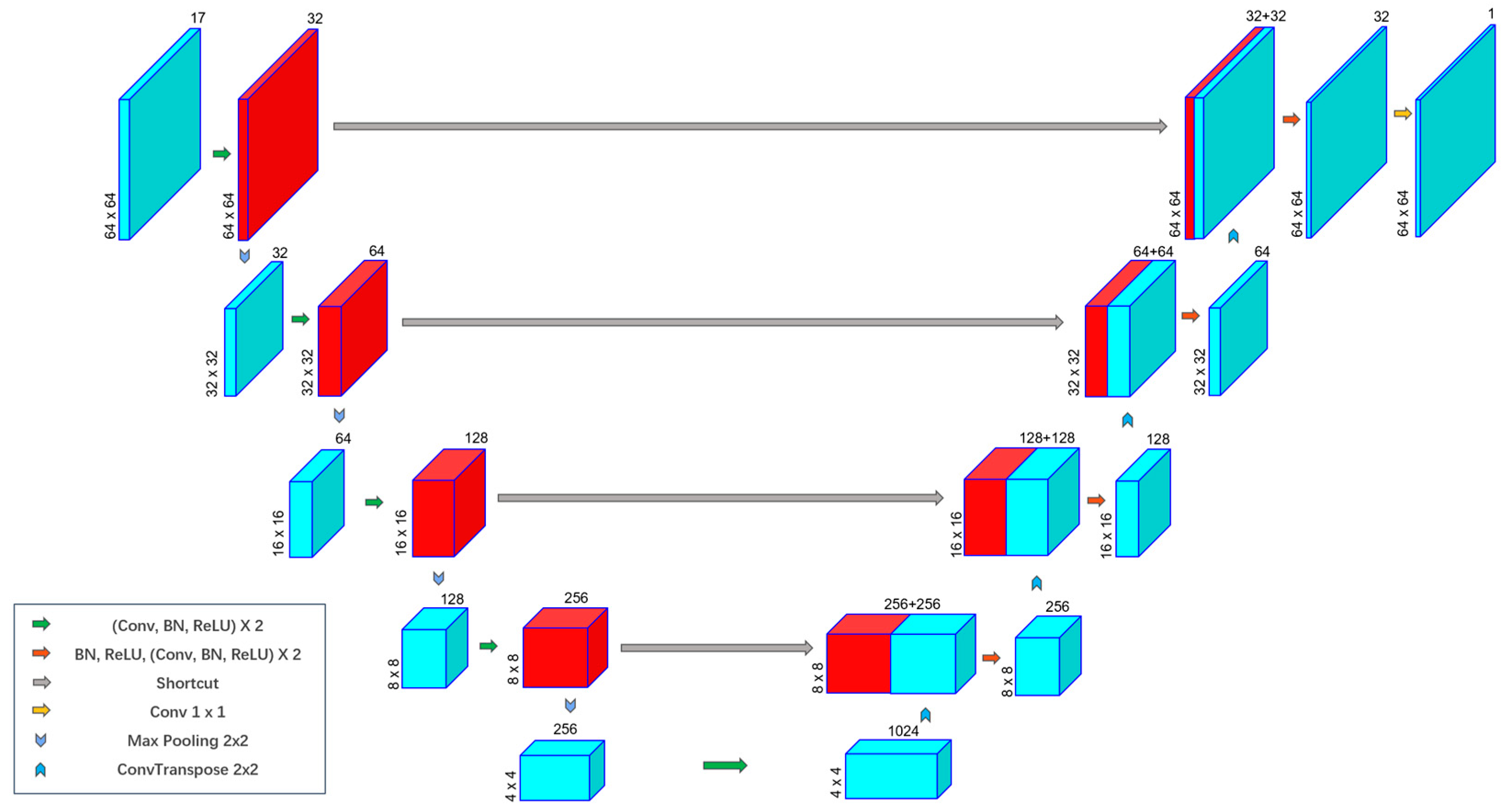
2.2.1. Satellite to Radar U-Net

U-Net has been shown to demonstrate good performance in the reconstruction of the radar data in previous studies [23,24,25,26,27]. We use the U-Net architecture to construct a CREF reconstruction model, namely satellite-to-radar U-Net (STR-UNet, Figure 1).
Overall, the STRU-Net designed in this study is of an encoder–decoder structure [27]. The left side of the network is often referred to as the contracting path and the right side is referred to as the expanding path. The shortcut in the middle is called the jump connection layer, which is also known as the feature splicing layer.
The left half of the model (contracting path) is used for feature extraction, which is repeatedly composed of convolution blocks and 2 × 2 pooling layers, and each convolution block contains the 3 × 3 convolution layer, batch normalization layer, and ReLU activation function. The input size of the model is a 64 × 64 × 17 satellite image, where 64 × 64 represents the length and width of the satellite image after padding, and 17 represents the number of input channels (i.e., bands). Then, after each convolution block and pooling, the number of feature maps is doubled and the length and width are halved, respectively.
The right half of the model (expanding path) performs the up-sampling operation, which is composed of several transposed convolution layers, feature splicing layers, and convolution blocks repeatedly, and the convolution block also encapsulates the batch normalization layer, 3 × 3 convolution layer, and ReLU activation function. In the expanding path, first we perform transposed convolution on the feature map obtained on the contracting path; next, the obtained feature map is spliced on the channel with the feature map at the corresponding position on the contracting path; then, the convolution operation is performed on the feature map after splicing, and so on and so forth. After each transposed convolution and convolution block, the number of feature maps is halved, and the length and width are doubled. In the last layer of the model, a 1 × 1 convolution layer maps the tensor of 32 channels to 1 channel, which in turn yields a target image of size 64 × 64 × 1. For this study, the reconstruction of CREF data is completed.
STRU-Net combines the low-resolution information in down-sampling process and high-resolution information in up-sampling process, and applies long-range jump connection combined with the feature details from the shallow convolution layer at the bottom of the satellite images, which can effectively compensate for the lack of spatial information of satellite images during the down-sampling process, and help the network to achieve more accurate localization. It is very important for reconstructing accurate radar data and boundary information.

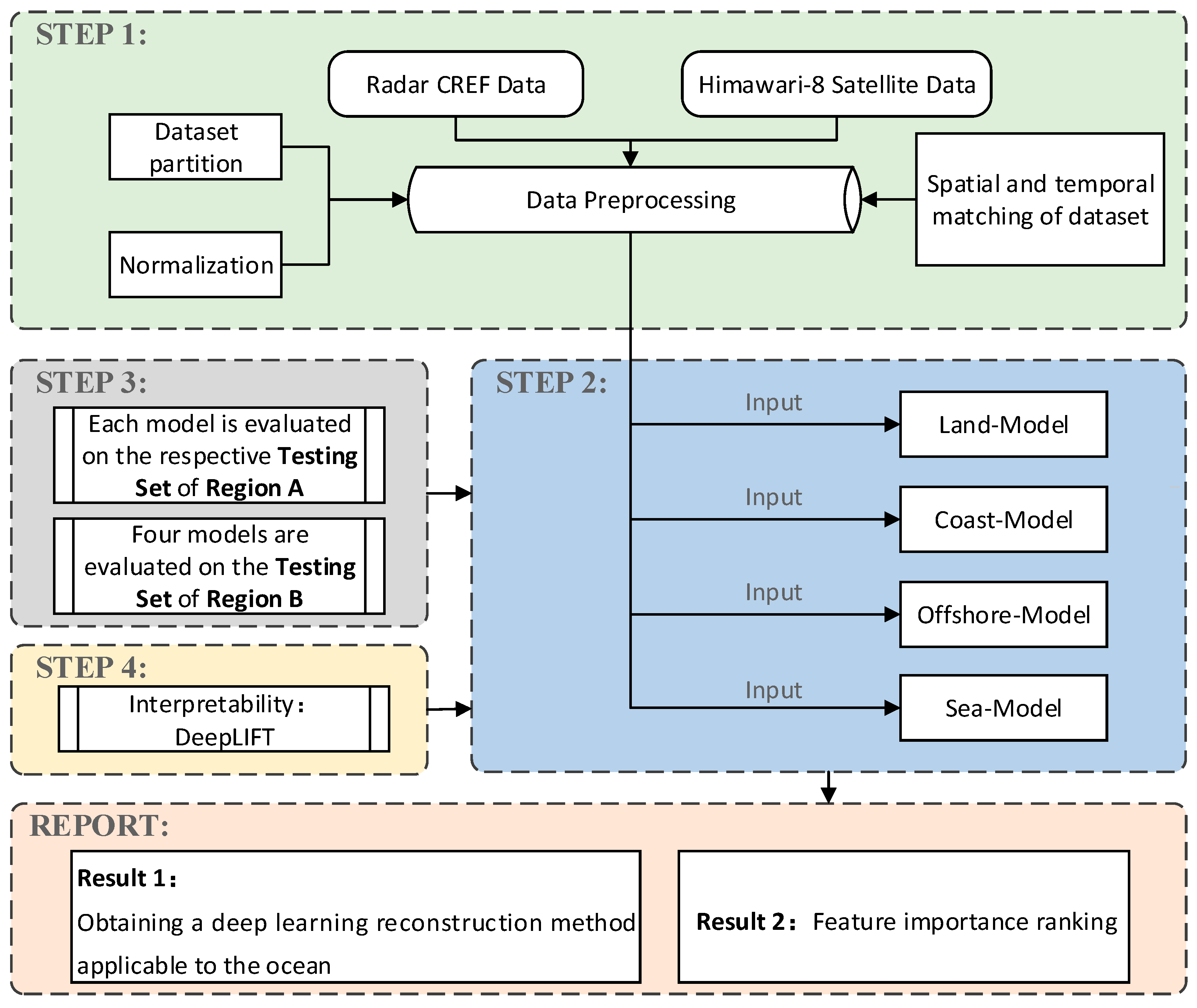
2.2.2. Research Scheme of the CREF Reconstruction

This paper aims to construct a satellite reconstruction model with satellite data that is suitable for monitoring severe convective weather in the ocean without deploying a radar. In order to achieve this objective, we designed the following research scheme, as shown in Figure 2.
Step 1. Preprocess the dataset, as described in Section 2.1.4.
Step 2. Build four STR-UNet models with different underlying surfaces. As shown in Figure 3 (Left), Region A includes four different underlying surfaces: land, coast, offshore, and sea. Four STR-UNet models, namely Land-Model, Coast-Model, Offshore-Model, and Sea-Model, are constructed.
Step 3. Train and test the STR-UNet models. The first 24 days of each month (May to October) in 2016 and 2017 are used as the training set, and the remaining days of these months are used as the validation set. The data in 2018 are used as the test set. It is worth noting that each model is trained and tested on its own underlying surface data. For example, the Coast-Model is trained and tested by using the data from the coastal area.
Then, the performances of the four STR-UNet models on the oceanic areas are assessed. The orange box regions, as shown in Figure 3 (Right), are defined as oceanic areas that are not overlapping with the “offshore” areas shown in Figure 3 (Left). It is difficult for us to obtain radar CREF from the ocean, and at this time, the offshore radar CREF has relatively high accuracy and its data comes from the ocean, which means it has data features of oceanic underlying surface. Based on this, we assume that Region B can represent the “ocean” underlying surface. The performance of the four models will be evaluated based on the test set (2018) in this area.
Step 4. Perform interpretability study of STR-UNet. See Section 2.2.4 for more details.

2.2.3. Evaluation Metrics

In this study, root mean square error (RMSE) and mean absolute error (MAE) are used to quantitatively verify the performance of the four STR-UNet models built in this paper. RMSE and MAE can measure the deviation between the reconstructed CREF and the radar CREF. The equations are as follows:
R M S E = 1 n i = 1 n y i - y i 2
M A E = 1 n i = 1 n y i - y i
where n represents the number of samples, y i represents the reconstructed CREF value, and y i represents the radar CREF value.
The classification metrics used in this study include probability of detection (POD), false alarm ratio (FAR), and critical success index (CSI), BIAS, as shown in Table 2. The model’s ability to reconstruct for CREF above 35 dBZ, a critical issue for many industries, including aviation and ship navigation, was evaluated using the classification criteria.
P O D = H i t s H i t s + M i s s e s
C S I = H i t s H i t s + M i s s e s + F a l s e   a l a r m s
B I A S = H i t s + F a l s e   a l a r m s H i t s + M i s s e s

2.2.4. Interpretability

In recent years, with the rapid development of deep learning, the interpretability of models has received more and more attention from scholars at home and abroad. Most deep learning models are “black box” models [40]. Their “black box” nature makes it difficult for scholars to understand the decision logic of the models in many cases, and thus they cannot fully trust the deep learning models. In order to improve the interpretability and transparency of deep learning models, this study investigates the interpretability of models.
For this study, a total of 17 features of satellite data were used as the input, after obtaining a model in different underlying surfaces, respectively, besides being interested in the effect of the model, it was essential to determine which features played an important role in the reconstruction.
In this paper, the DeepLIFT algorithm is used to conduct interpretability research on the above models. The DeepLIFT [36] method allocates the prediction results of the neural network to each dimension of the input. Its working principle is to compare the activation of each neuron with its “reference” activation, and back propagate the importance signal in order to assign a contribution score based on the difference. In essence, this is a method of tracing the internal feature selection of the algorithm, which uses the input differences of some “reference” inputs to explain the output differences of some “reference” outputs.
In this study, for each band feature, first, we conducted the normalization on Region B, and the vector with the “reference” value of all zeros was set to calculate the attribution of each feature, which is the contribution of each input feature to the results. Finally, the absolute value of attribution was taken, and the ratio of the absolute value of each feature attribution to the sum of the absolute values of all feature attributions was expressed as the importance of the feature.
Based on this method, several more important features on different underlying surfaces can be selected, and whether surface information affects the band selection of the model can be analyzed. Finally, we explored the relationship between the importance of bands and underlying surfaces, as well as the reasons why different underlying surfaces differed in importance.

3. Results

3.1. Performances of the Four STR-UNet Models
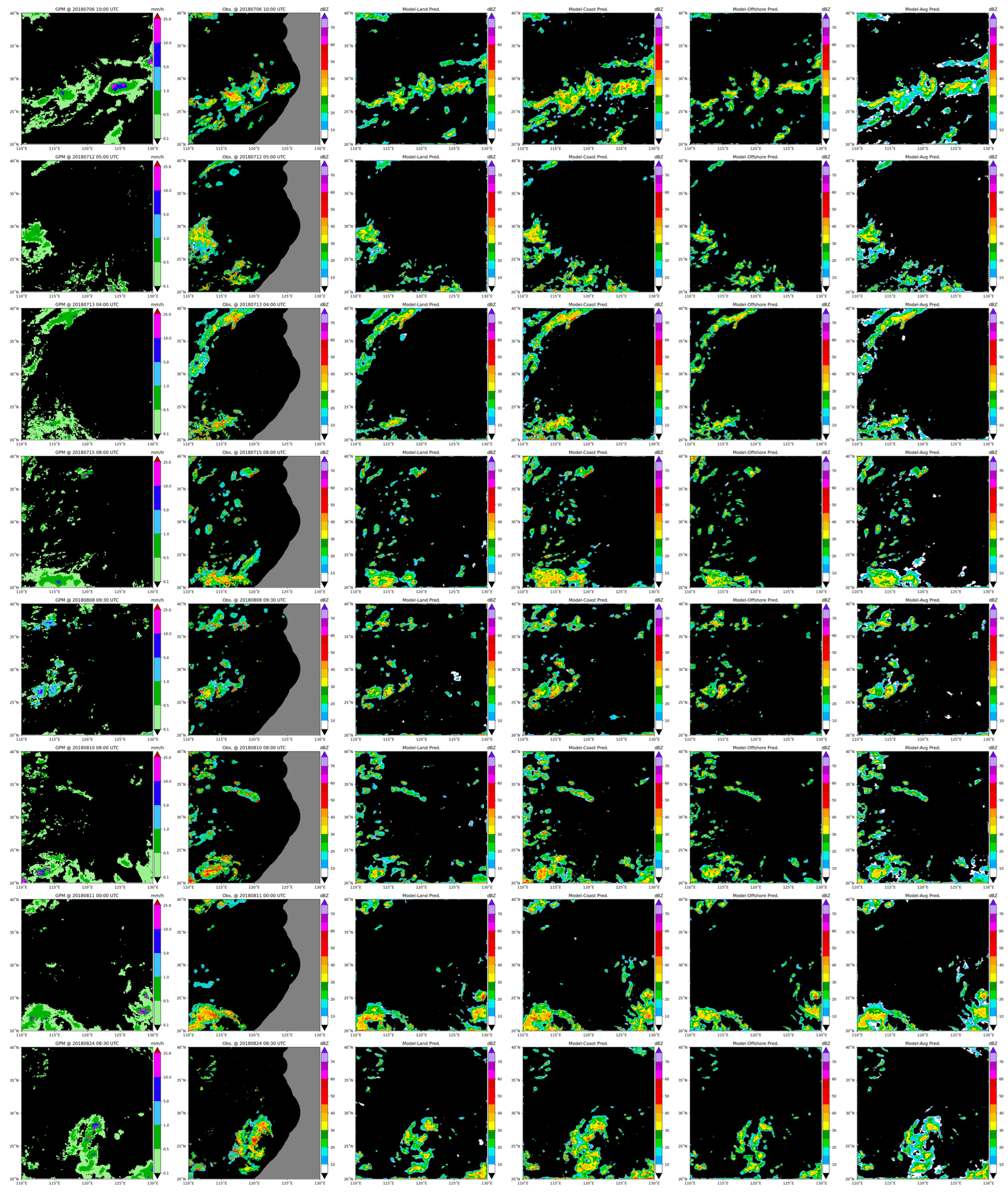
The performances of the four STR-UNet models are shown in Table 3.
First, in the process of advancing from land to coast, to offshore, and then to ocean, it can be found that the RMSE and MAE are getting smaller on the test set in Region A. However, it does not indicate that the model’s performance is getting better. The main reason is that the CREF refers to the ratio of the radar waves reflected from clouds of different heights within a certain range received by the meteorological radar. With the increasing distance from the coastline to the ocean, the radiation elevation of the radar is also increasing. It means that at a distance from the radar, the CREF is only calculated based on a small number of basic reflectivity factors of higher elevations. As a result, the proportion of CREF larger than 35 dBZ decreases significantly as one moves from land to coast, offshore, and finally to the ocean, as depicted in Figure 4. Especially for the sea areas in Region A, the proportion of CREF larger than 35 dBZ is only a few tenths of that of the other three areas.
Then, we observe the performance of the four models on the test set in Region B. For all the metrics, it can be seen that when the models are evaluated in Region B, the performances of the Land-Model, Coast-Model, and Offshore-Model are significantly better than those of Sea-Model. Four metrics (POD, CSI, BIAS and FAR) of the Sea-Model are 0, and the RMSE and MAE are the largest among all these models. It indicates that the Sea-Model does not have the ability to reconstruct the CREF.
Since the Offshore-Model’s data selection resembles that of Region B (without overlap), it can serve as a proxy for the highest level of precision that the reconstruction model is capable of. Compared to the Offshore-Model, the Land-Model’s performances are a little worse on the test set in Region B for all the evaluation metrics.
It is a little complicated to evaluate the performance of the Coast-Model compared to the Offshore-Model. The RMSE, MAE, and FAR of the Coast-Model are a little larger (worse) than those of Offshore-Model. However, the Coast-Model has better POD, CSI, and BIAS than the Offshore-Model. This is due to the fact that, as shown in Figure 4, the coastal area has the highest fraction of CREF larger than 35 dBZ compared to the other three areas. It denotes a complicated meteorological situation affected by the complex underlying surface of the coast [41,42]. Thus, compared to the Offshore-Model, the prediction of Coast-Model is bolder.
In conclusion, a mix of land-dataset, coast-dataset, and offshore-dataset can be taken into consideration when employing satellite data to reconstruct radar data. The Offshore-Model can give the medium results, while the Coast-Model can give bolder results. Due to the abundance of data on land area, the Land-Model can provide a good baseline for reconstructing the radar data, despite being slightly inferior to the Offshore-Model on the test set in Region B.

3.2. Case Study

In order to demonstrate the actual combat effect of the models, we selected several severe convective weather cases from the test set (UTC) to visually show the reconstruction effect of the models.
Typhoon is one of the important disastrous weather systems that affects the safety of people’s lives and property. It often brings rainstorm, strong wind, and secondary disasters [43]. Typhoon “Yagi” was generated on 7 August 2018 (Beijing time, the same below) with the intensity of a tropical depression. The intensity of “Yagi” increased to a tropical storm on 8 August, moving towards the north by east, turning to the northwest at night on 9 August, and entering the eastern region of the East China Sea at night on 11 August [44]. During the influence of “Yagi”, extreme precipitation and a large-scale rainstorm had been brought to the cities along the way, resulting in heavy economic losses. Figure 5 shows the GPM precipitation and radar echo distribution of severe convective events that occurred in the research area in the test set. It can be seen that the models can more accurately reconstruct the shape, location, intensity, and range of the convective center, whether it is a slightly lower intensity convective event or a severe convective event such as a typhoon. In addition, for areas beyond the radar coverage, the radar echoes can be also reconstructed, and the distribution of reconstructed CREF is quite consistent with the pattern of the GPM precipitation.

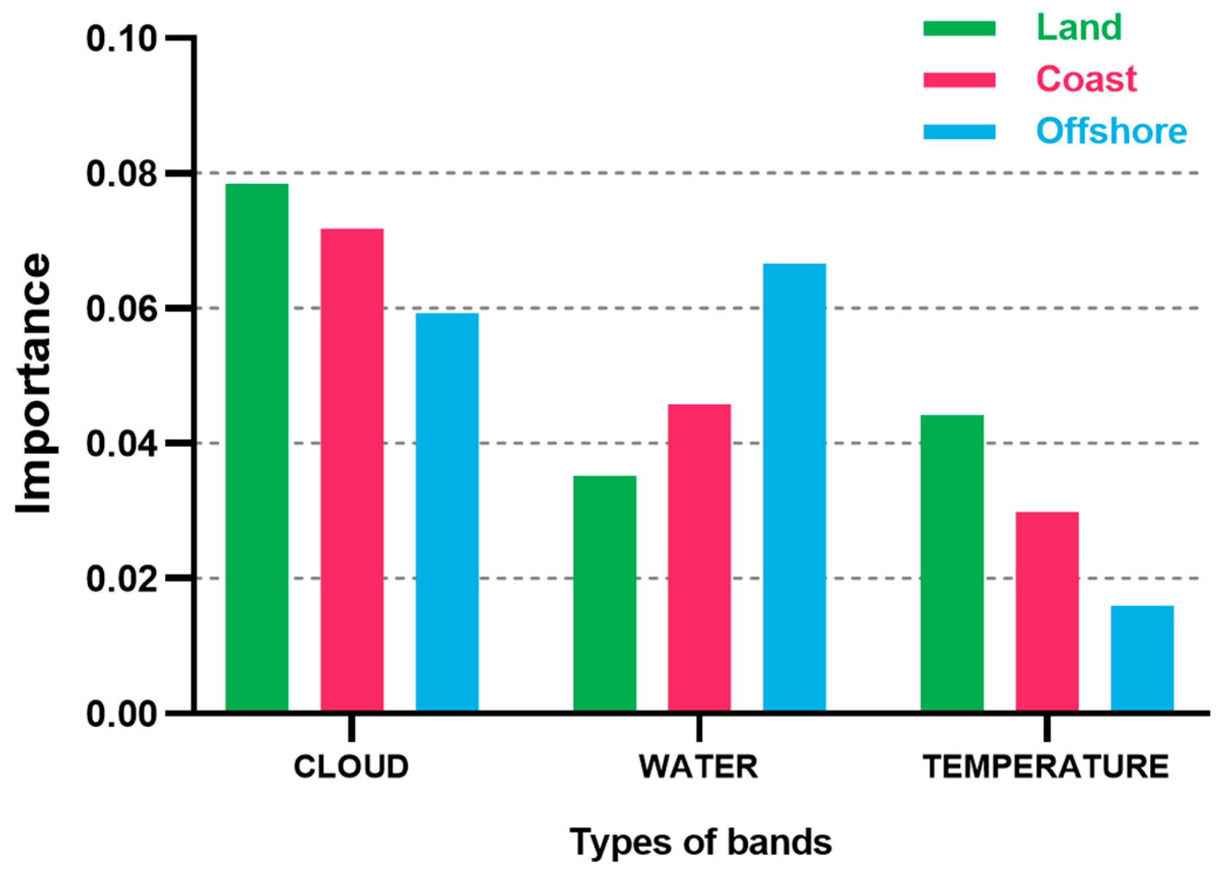
3.3. Results of Interpretability

For the models selected above: Land-Model, Coast-Model and Offshore-Model, the DeepLIFT method is adopted to analyze the differences in feature importance under different underlying surfaces (land, coast, and offshore). The results are shown in Figure 6.
According to the previous description, and their physical meaning (Table 1), the 17 input features of satellite bands can be classified as satellite cloud-related features, satellite water-related features, and satellite temperature-related features. It is worth mentioning that for bands with more than one type of physical meaning, such as Band 11, the center wavelength is 8.6 μm, which can both measure water vapor and cloud phase state. When classifying the input features, Band 11 is classified as both satellite water-related features and satellite cloud-related features. It means that after calculating the importance of Band 11 using the DeepLIFT method, we will calculate the average importance of satellite water-related features along with other bands that measure water vapor. At the same time, the importance of Band 11 will be used along with bands that measure the cloud phase state to calculate the average importance of satellite cloud-related features. Similarly, we calculated the average value of the importance of the bands under each type. For the land’s underlying surface, it can be intuitively seen that satellite cloud-related features are more important to the reconstruction, far outweighing the importance of satellite water-related features and satellite temperature-related features.
Overall, satellite cloud-related features are the most important, followed by satellite water-related features, and satellite temperature-related features are the least important. When the underlying surface changes to the coast, then to the offshore, the importance of satellite cloud-related features gradually decreases, but they still play an important role in reconstruction, while the importance of satellite water-related features gradually increases, which is also important for reconstruction. When the underlying surface is located on the ocean, it is clear that satellite water-related features are more important than satellite cloud-related features. The importance of satellite temperature-related features gradually decreases as the model changes to the ocean, compared with the former two, they are relatively unimportant in reconstruction.
In summary, during the transition of the model from the land to the ocean, for all the underlying surface cases, clouds have a great impact on the amount of solar radiation reaching the Earth and play a crucial role in the water cycle of the climate system [45,46]; the cloud phase state can also reflect the temperature and humidity state, and dynamic characteristics of the atmosphere to a certain extent [47]. In addition, water vapor has a strong correlation with severe convective weather; the increase in water vapor content is conducive to the development of convective weather and it can easily cause the rapid growth of convective weather. Therefore, the satellite features characterizing cloud amount, cloud phase state, and water vapor play an important role in reconstruction. Secondly, for the underlying surface of the ocean, because the ocean has the characteristics of high heat capacity and high thermal inertia, it means that it needs more energy to make its temperature change greatly. Therefore, compared with the land’s underlying surface, satellite temperature-related features have a lower significance in the reconstruction of severe convective weather.

4. Conclusions

In this study, we, respectively, sampled land, coast, offshore, and sea areas in the eastern area (20°N–40°N, 110°E–130°E), built four deep learning models using U-Net, and compared their accuracy. The results show that a mix of land-dataset, coast-dataset, and offshore-dataset can be taken into consideration when deploying satellite data to reconstruct radar data. This allows for more accurate reconstruction and monitoring of severe convective weather in the ocean without radar deployment.
In addition, in previous studies, there was a lack of research on the interpretability of the models. In this paper, the DeepLIFT method was used to obtain the feature importance ranking and the differences in different underlying surfaces. Overall, satellite cloud-related features are most important, followed by satellite water-related features, and satellite temperature-related features are the least important. The importance of satellite water-related features gradually increases, and the importance of satellite cloud-related features and satellite temperature-related features gradually decreases as the model changes from land to ocean. Then, the reasons for this phenomenon are briefly analyzed in combination with physical meaning. It is beneficial to the research in the oceanic area, which is of great significance for aviation, navigation, and the maintenance of people’s lives and property safety.
In addition to the research tasks outlined in this study, future research will be conducted from the following aspects.
Firstly, the data used in this paper are infrared band data, while the data used in previous studies include lightning and other data. In subsequent studies, we will also increase the data types in order to further reduce the error and improve the reconstruction effect. Secondly, we used the DeepLIFT method to preliminarily analyze the differences in feature importance caused by the differences in the underlying surfaces of the model. However, using only one method to study the interpretability means the results lack credibility [48]. In the future, we will use more interpretable methods and optimize them to obtain more convincing interpretable conclusions. We hope the reconstruction method we have proposed will spur new developments in the deep learning and meteorological fields.

Author Contributions

Conceptualization, X.Y., J.X. and D.Z.; methodology, X.L., X.Y., Y.Y., J.X. and Z.W.; software, X.L., W.C., X.Y. and Y.Y.; validation, X.Y. and X.L.; formal analysis, X.Y.; resources, J.X. and Z.Y.; data curation, X.L. and X.Y.; writing—original draft preparation, X.Y. and J.X.; writing—review and editing, Z.Y., Y.Y., W.C., Z.W. and D.Z.; visualization, X.Y. and X.L. All authors have read and agreed to the published version of the manuscript.

Funding

This study was funded by the National Natural Science Foundation of China (Grant No. 42275158).

Data Availability Statement

Not applicable.

Acknowledgments

We would like to express our gratitude to the Japan Meteorological Agency (JMA) for freely providing the Himawari-8 satellite data used in this research.

Conflicts of Interest

The authors declare no conflict of interest.

References

  1. Maddox, R.A. Mesoscale convective complexes. Bull. Am. Meteorol. Soc. 1980, 61, 1374–1387. [Google Scholar] [CrossRef]
  2. Brimelow, J.C.; Hanesiak, J.M.; Burrows, W.R. On the Surface-Convection Feedback during Drought Periods on the Canadian Prairies. Earth Interact. 2011, 15, 1–26. [Google Scholar] [CrossRef]
  3. Zheng, Y.; Tian, F.; Meng, Z.; Xue, M.; Yao, D.; Bai, L.; Zhou, X.; Mao, X.; Wang, M. Survey and Multi-Scale Characteristics of Wind Samage Caused by Convective Storms in the Surrounding Area of the Capsizing Accident of Cruise Ship “Dongfangzhixing”. Meteorol. Mon. 2016, 42, 1–13. (In Chinese) [Google Scholar]
  4. Zheng, Y.; Zhou, K.; Sheng, J.; Lin, Y.; Tian, F.; Tang, W.; Lan, Y.; Zhu, W. Advances in Techniques of Monitoring, Forecasting and Warning of Severe Convective Weather. J. Appl. Meteorol. Sci. 2015, 26, 641–657. (In Chinese) [Google Scholar]
  5. Roberts, R.D.; Rutledge, S. Nowcasting storm initiation and growth using GOES-8 and WSR-88D data. Weather Forecast. 2003, 18, 562–584. [Google Scholar] [CrossRef]
  6. Stampoulis, D.; Anagnostou, E.N. Evaluation of global satellite rainfall products over continental Europe. J. Hydrometeorol. 2012, 13, 588–603. [Google Scholar] [CrossRef]
  7. Arkin, P.A.; Meisner, B.N. The relationship between large-scale convective rainfall and cold cloud over the Western Hemisphere during 1982–1984. Mon. Weather Rev. 1987, 115, 51–74. [Google Scholar] [CrossRef]
  8. Arkin, P.A.; Joyce, R.; Janowiak, J.E. The estimation of global monthly mean rainfall using infrared satellite data: The GOES Precipitation Index (GPI). Remote Sens. Rev. 1994, 11, 107–124. [Google Scholar] [CrossRef]
  9. Liu, Y.; Fu, Q.; Song, P. Satellite retrieval of precipitation: An overview. Adv. Atmos. Sci. 2011, 26, 1162–1172. (In Chinese) [Google Scholar]
  10. Bastiaanssen, W.G.M.; Pelgrum, H.; Wang, J.; Ma, Y.; Moreno, J.F.; Roerink, G.J.; van der Wal, T. A remote sensing surface energy balance algorithm for land (SEBAL): Part 2: Validation. J. Hydrol. 1998, 212, 213–229. [Google Scholar] [CrossRef]
  11. Liang, L.; Liu, C.; Xu, Y.Q.; Guo, B.; Shum, H.Y. Real-time texture synthesis by patch-based sampling. ACM Trans. Graph. 2001, 20, 127–150. [Google Scholar] [CrossRef]
  12. Scofield, R.A.; Kuligowski, R.J. Status and Outlook of Operational Satellite Precipitation Algorithms for Extreme-Precipitation Events. Weather Forecast. 2003, 18, 1037–1051. [Google Scholar] [CrossRef]
  13. Ba, M.B.; Gruber, A. GOES Multispectral Rainfall Algorithm (GMSRA). J. Appl. Meteor. Climatol. 2001, 40, 1500–1514. [Google Scholar] [CrossRef]
  14. Zhang, Y.; Wu, K.; Zhang, J.; Zhang, F.; Xiao, H.; Wang, F.; Zhou, J.; Song, Y.; Peng, L. Estimating Rainfall with Multi-Resource Data over East Asia Based on Machine Learning. Remote Sens. 2021, 13, 3332. [Google Scholar] [CrossRef]
  15. Chang, G.W.; Lu, H.J.; Chang, Y.R.; Lee, Y.D. An improved neural network-based approach for short-term wind speed and power forecast. Renew. Energ. 2017, 105, 301–311. [Google Scholar] [CrossRef]
  16. Beusch, L.; Foresti, L.; Gabella, M.; Hamann, U. Satellite-Based Rainfall Retrieval: From Generalized Linear Models to Artificial Neural Networks. Remote Sens. 2018, 10, 939. [Google Scholar] [CrossRef] [Green Version]
  17. Hsu, K.; Gao, X.; Sorooshian, S.; Gupta, H.V. Precipitation Estimation from Remotely Sensed Information Using Artificial Neural Networks. J. Appl. Meteor. Climatol. 1997, 36, 1176–1190. [Google Scholar] [CrossRef]
  18. Hong, Y.; Hsu, K.L.; Sorooshian, S.; Gao, X. Precipitation estimation from remotely sensed imagery using an artificial neural network cloud classification system. J. Appl. Meteorol. 2004, 43, 1834–1853. [Google Scholar] [CrossRef] [Green Version]
  19. Krizhevsky, A.; Sutskever, I.; Hinton, G.E. ImageNet classification with deep convolutional neural networks. Commun. ACM. 2012, 60, 84–90. [Google Scholar] [CrossRef] [Green Version]
  20. Veillette, M.S.; Hassey, E.P.; Mattioli, C.J.; Iskenderian, H.; Lamey, P.M. Creating Synthetic Radar Imagery Using Convolutional Neural Networks. J. Atmos. Ocean. Technol. 2018, 35, 2323–2338. [Google Scholar] [CrossRef]
  21. Wang, C.; Xu, J.; Tang, G.; Yang, Y.; Hong, Y. Infrared Precipitation Estimation Using Convolutional Neural Network. IEEE Trans. Geosci. Remote Sens. 2020, 58, 8612–8625. [Google Scholar] [CrossRef]
  22. Ronneberger, O.; Fischer, P.; Brox, T. 2015: U-Net: Convolutional Networks for Biomedical Image Segmentation. In Proceedings of the 18th International Conference on Medical Image Computing and Computer-Assisted Intervention-MICCAI, Munich, Germany, 5–19 November 2015; Springer: Cham, Switzerland, 2015; pp. 234–241. [Google Scholar]
  23. Hilburn, K.A.; Ebert-Uphoff, I.; Miller, S.D. Development and Interpretation of a Neural Network-Based Synthetic Radar Reflectivity Estimator Using GOES-R Satellite Observations. J. Appl. Meteor. Climatol. 2020, 60, 1–21. [Google Scholar] [CrossRef]
  24. Duan, M.; Xia, J.; Yan, Z.; Han, L.; Zhang, L.; Xia, H.; Yu, S. Reconstruction of the Radar Reflectivity of Convective Storms Based on Deep Learning and Himawari-8 Observations. Remote Sens. 2021, 13, 3330. [Google Scholar] [CrossRef]
  25. Sun, F.; Li, B.; Min, M.; Qin, D. Deep Learning-Based Radar Composite Reflectivity Factor Estimations from Fengyun-4A Geostationary Satellite Observations. Remote Sens. 2021, 13, 2229. [Google Scholar] [CrossRef]
  26. Yang, L.; Zhao, Q.; Xue, Y.; Sun, F.; Li, J.; Zhen, X.; Lu, T. Radar Composite Reflectivity Reconstruction Based on FY-4A Using Deep Learning. Sensors. 2023, 23, 81. [Google Scholar] [CrossRef]
  27. Veillette, M.; Samsi, S.; Mattioli, C. Sevir: A storm event imagery dataset for deep learning applications in radar and satellite meteorology. Adv. Neural Inf. Process. Syst. 2020, 33, 22009–22019. [Google Scholar]
  28. Zhang, P.; Du, B.; Dai, T. Radar Meteorology, 2nd ed.; China Meteorological Press: Beijing, China, 2010. [Google Scholar]
  29. Van Lent, M.; Fisher, W.; Mancuso, M. An explainable artificial intelligence system for small-unit tactical behavior. In Proceedings of the National Conference on Artificial Intelligence, San Jose, CA, USA, 25–29 July 2004; AAAI Press: Menlo Park, CA, USA; MIT Press: Cambridge, MA, USA; London, UK, 1999; pp. 900–907. [Google Scholar]
  30. Ribeiro, M.T.; Singh, S.; Guestrin, C. “Why Should I Trust You?” Explaining the Predictions of Any Classifier. In Proceedings of the 22nd ACM SIGKDD International Conference on Knowledge Discovery and Data Mining, New York, NY, USA, 13–17 August 2016; pp. 1135–1144. [Google Scholar]
  31. Bach, S.; Binder, A.; Montavon, G.; Klauschen, F.; Müller, K.-R.; Samek, W. On Pixel-Wise Explanations for Non-Linear Classifier Decisions by Layer-Wise Relevance Propagation. PLoS ONE 2015, 10, e0130140. [Google Scholar] [CrossRef] [Green Version]
  32. Lundberg, S.M.; Lee, S.-I. A unified approach to interpreting model predictions. Adv. Neural Inf. Process. Syst. 2017, 30, 4768–4777, ArXiv:1705.07874. [Google Scholar]
  33. Selvaraju, R.R.; Cogswell, M.; Das, A.; Vedantam, R.; Parikh, D.; Batra, D. Grad-CAM: Visual Explanations from Deep Networks via Gradient-based Localization. Int. J. Comput. Vis. 2020, 128, 336–359. [Google Scholar] [CrossRef] [Green Version]
  34. Cho, K.; van Merriënboer, B.; Gulcehre, C.; Bahdanau, D.; Bougares, F.; Schwenk, H.; Bengio, Y. Learning phrase representations using RNN encoder-decoder for statistical machine translation. In Proceedings of the 2014 Conference on Empirical Methods in Natural Language Processing (EMNLP), Doha, Qatar, 26–28 October 2014; pp. 1724–1734. [Google Scholar]
  35. Zhou, Y.; Wang, H.; Zhao, J.; Chen, Y.; Yao, R.; Chen, S. Interpretable attention part model for person re-identification. Acta Autom. Sin. 2020, 41, 116. (In Chinese) [Google Scholar]
  36. Shrikumar, A.; Greenside, P.; Kundaje, A. Learning important features through propagating activation differences. In Proceedings of the 34th International Conference on Machine Learning. PMLR, Sydney, Australia, 6–11 August 2017; pp. 3145–3153. [Google Scholar]
  37. Yasuhiko, S.; Hiroshi, S.; Takahito, I.; Akira, S. Convective Cloud Information derived from Himawari-8 data. In Meteorological Satellite Center Technical Note; Meteorological Satellite Center (MSC): Kiyose, Tokyo, 2017; p. 22. [Google Scholar]
  38. Sun, S.; Li, W.; Huang, Y. Retrieval of Precipitation by Using Himawari-8 Infrared Images. Acta Sci. Nat. Univ. Pekinensis 2019, 55, 215–226. (In Chinese) [Google Scholar]
  39. Sadeghi, M.; Asanjan, A.A.; Faridzad, M.; Nguyen, P.; Hsu, K.; Sorooshian, S.; Braithwaite, D. PERSIANN-CNN: Precipitation Estimation from Remotely Sensed Information Using Artificial Neural Networks–Convolutional Neural Networks. J. Hydrometeor. 2019, 20, 2273–2289. [Google Scholar] [CrossRef]
  40. Bathaee, Y. The Artificial Intelligence Black Box and the Failure of Intent and Causation. Harvard J. Law Technol. 2018, 31, 889. [Google Scholar]
  41. Zhai, G.; Ding, H.; Gao, K. A Numerical Experiment of the Meso-scale Influence of Underlying Surface on a Cyclonic Precipitation Process. J. Hangzhou Univ. (Nat. Sci.) 1995, 22, 185–190. (In Chinese) [Google Scholar]
  42. Tian, C.; Zhou, W.; Miao, J. Review of lmpact of Land Surface Characteristics on Severe Convective Weather in China. Meteorol. Sci. Technol. 2012, 40, 207–212. (In Chinese) [Google Scholar]
  43. Lyu, X.; Xu, Y.; Dong, L.; Gao, S. Analysis of characteristics and forecast difficulties of TCs over Northwestern Pacific in 2018. Meteor. Mon. 2021, 47, 359–372. (In Chinese) [Google Scholar]
  44. Sun, S.; Chen, B.; Sun, J.; Sun, Y.; Diao, X.; Wang, Q. Periodic Characteristics and Cause Analysis of Continuous Heavy Rainfall Induced by Typhoon Yagi (1814) in Shandong. Plateau Meteorol. 2022, 1–15. (In Chinese) [Google Scholar] [CrossRef]
  45. Zhang, Q.; Li, Y.; Yang, Y. Research Progress on the Cloudage and Its Relation with Precipitation in China. Plateau Mt. Meteorol. Res. 2011, 31, 79–83. (In Chinese) [Google Scholar]
  46. Zou, Y.; Wang, Y.; Wang, S. Characteristics of lighting activity during severe convective weather in Dalian area based on satellite data. J. Meteorol. Environ. 2021, 37, 128–133. (In Chinese) [Google Scholar]
  47. Cao, Z.; Wang, X. Cloud Characteristics and Synoptic Background Associated with Severe Convective Storms. J. Appl. Meteorol. Sci. 2013, 24, 365–372. (In Chinese) [Google Scholar]
  48. McGovern, A.; Lagerquist, R.; Gagne, D.J.; Jergensen, G.E.; Elmore, K.L.; Homeyer, C.R.; Smith, T. Making the black box more transparent: Understanding the physical implications of machine learning. Nat. Mach. Intell. 2019, 100, 2175–2199. [Google Scholar] [CrossRef]
Figure 1. The STR-UNet architecture.
Remotesensing 15 03065 g001
Figure 2. Research scheme of the CERF reconstruction.
Remotesensing 15 03065 g002
Figure 3. Schematic diagram of Region A (left) and Region B (right). Region A includes four different underlying surfaces: land (yellow box), coast (green box), offshore (cyan box), and sea (blue box). Region B only includes one underlying surface: offshore, and it does not coincide with the four underlying surfaces of Region A.
Remotesensing 15 03065 g003
Figure 4. Probability statistics of CREF data in different regions. The horizontal axis represents the range of CREF values, while the vertical axis represents the corresponding proportion. The different colors on the figure correspond to different underlying surfaces.
Remotesensing 15 03065 g004
Figure 5. Radar echo map: comparative study of observation and reconstruction. The first column shows GPM precipitation distribution at different times; the second column shows the radar echo observed; the gray areas on the map represent areas outside the radar deployment range. The third, fourth, and fifth columns show the reconstructions of the Land-Model, Coast-Model, and Offshore-Model, respectively, and the last column represents the average of the three reconstructed models mentioned above.
Remotesensing 15 03065 g005
Figure 6. The importance of each type of band (cloud, water, and temperature) under different underlying surfaces (land, coast, offshore).
Remotesensing 15 03065 g006
Table 1. 17 satellite bands selected or calculated in this study, along with physical meaning of each band. ‘-’ indicates minus. E.g., tbb08-tbb10 (Band 08 minus Band10) indicates the BTDs between band 08 and band 10.
BandCentral WavelengthPhysical MeaningType
Band 073.9Shortwave infrared window, low clouds, fogCloud
Band 086.2Mid and high level water vaporWater
Band 096.9Middle level water vaporWater
Band 107.3Middle and low level water vaporWater
Band 118.6Water vapor, Cloud phase stateWater, Cloud
Band 1310.4Cloud imagingCloud
Band 1411.2Surface temperatureTemperature
Band 1512.4Surface temperatureTemperature
Band 1613.3Temperature, Cloud top heightTemperature, Cloud
Band 08-146.2–11.2Temperature, Cloud top heightTemperature, Cloud
Band 10-157.3−12.4Temperature, Cloud top heightTemperature, Cloud
Band 08-106.2–7.3Water vapor detection above cloud topWater
Band 08-136.2−10.4Water vapor detection above cloud topWater
Band 11-148.6−11.2Cloud phase stateCloud
Band 14-1511.2−12.4Cloud phase stateCloud
Band 13-1510.4–12.4Detection of ice cloudCloud
Band 13-1610.4–13.3Detection of ice cloudCloud
Table 2. Contingency table of the classification score parameters.
Reconstructed CREF (<35 dBZ)Reconstructed CREF (≥35 dBZ)
True CREF (<35 dBZ)Correct negativesFalse alarms
True CREF (≥35 dBZ)MissesHits
Table 3. Performances of the four STR-UNet models.
ModelMetricRegion A Test
(on Each of the Four Underlying Surfaces, Respectively)
Region B Test
(Ocean)
Land-ModelRMSE7.43925.6120
MAE3.23531.8542
POD (35 dBZ)0.14780.1815
CSI (35 dBZ)0.12740.1484
FAR (35 dBZ)0.51950.5509
BIAS (35 dBZ)0.30760.4042
Coast-ModelRMSE7.15176.0755
MAE3.03152.1929
POD (35 dBZ)0.26630.2954
CSI (35 dBZ)0.21770.1958
FAR (35 dBZ)0.45600.6327
BIAS (35 dBZ)0.48950.8042
Offshore-ModelRMSE5.08245.0591
MAE1.46461.4444
POD (35 dBZ)0.21070.2144
CSI (35 dBZ)0.17550.1703
FAR (35 dBZ)0.48790.5469
BIAS (35 dBZ)0.41150.4732
Sea-ModelRMSE4.17447.7300
MAE0.70192.1525
POD (35 dBZ)0.00000.0000
CSI (35 dBZ)0.00000.0000
FAR (35 dBZ)0.00000.0000
BIAS (35 dBZ)0.00000.0000
Disclaimer/Publisher’s Note: The statements, opinions and data contained in all publications are solely those of the individual author(s) and contributor(s) and not of MDPI and/or the editor(s). MDPI and/or the editor(s) disclaim responsibility for any injury to people or property resulting from any ideas, methods, instructions or products referred to in the content.

