

Determination of the Stability of a High and Steep Highway Slope in a Basalt Area Based on Iron Staining Anomalies

Abstract
:1. Introduction
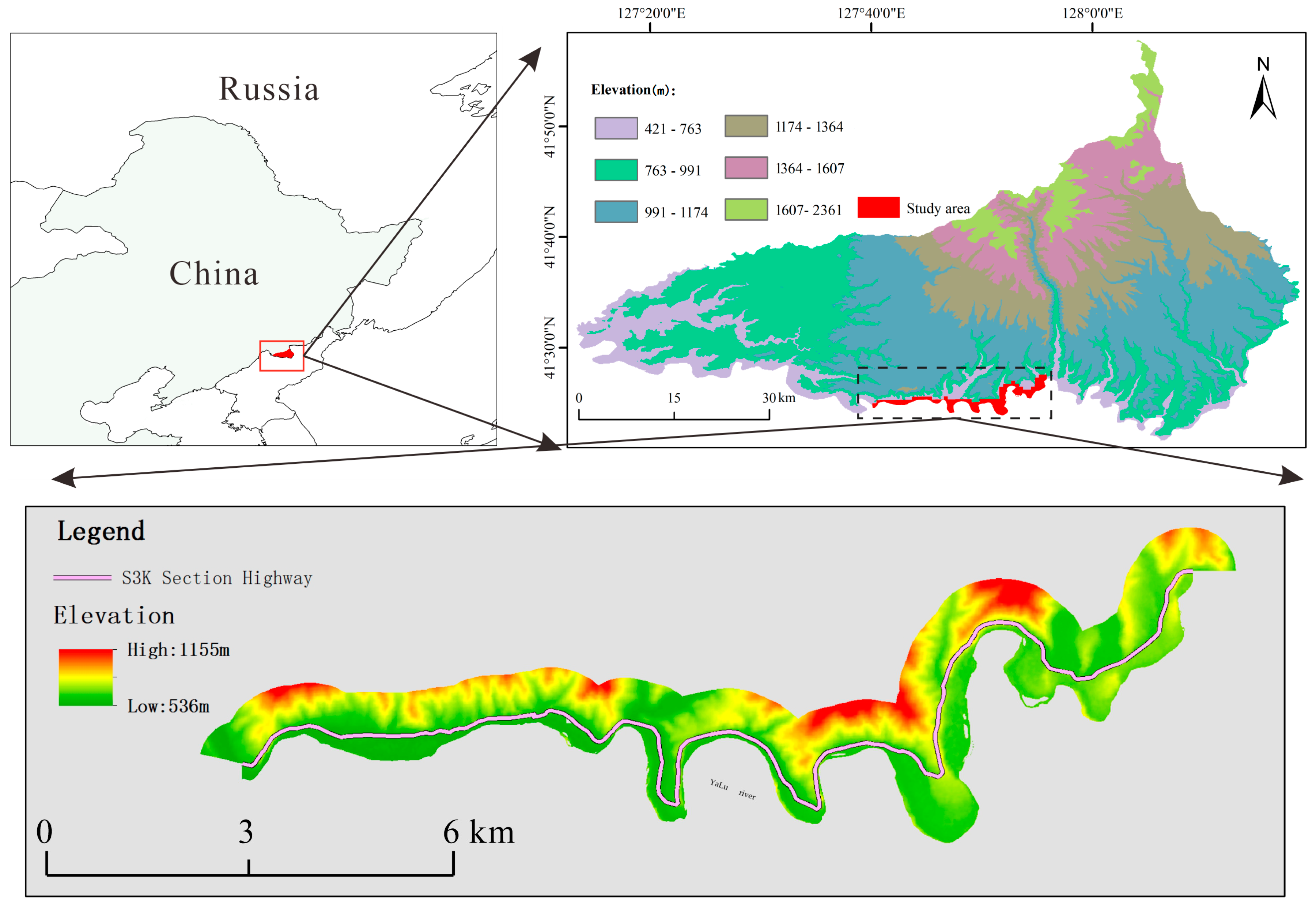
2. Study Area
3. Theory and Methods
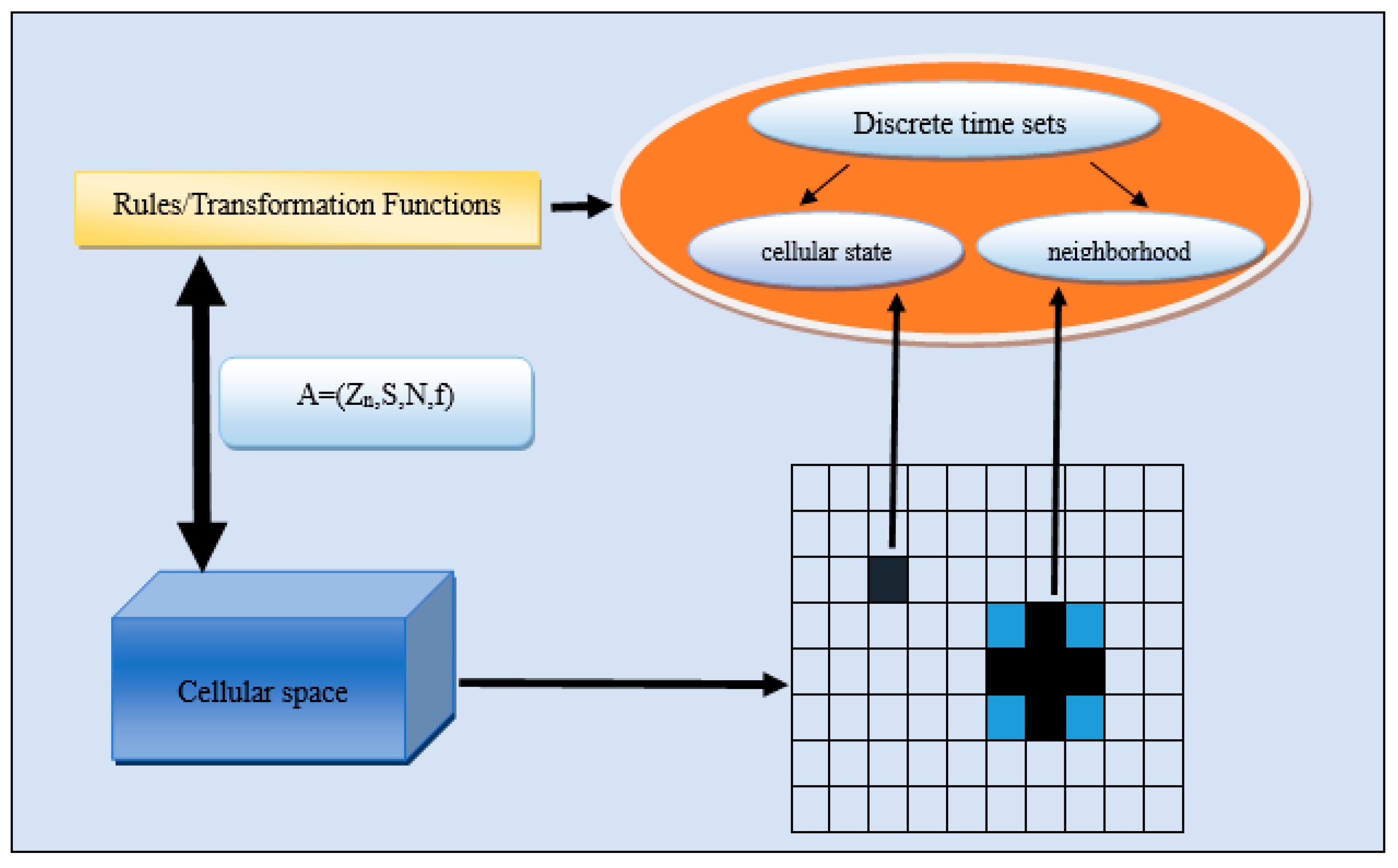
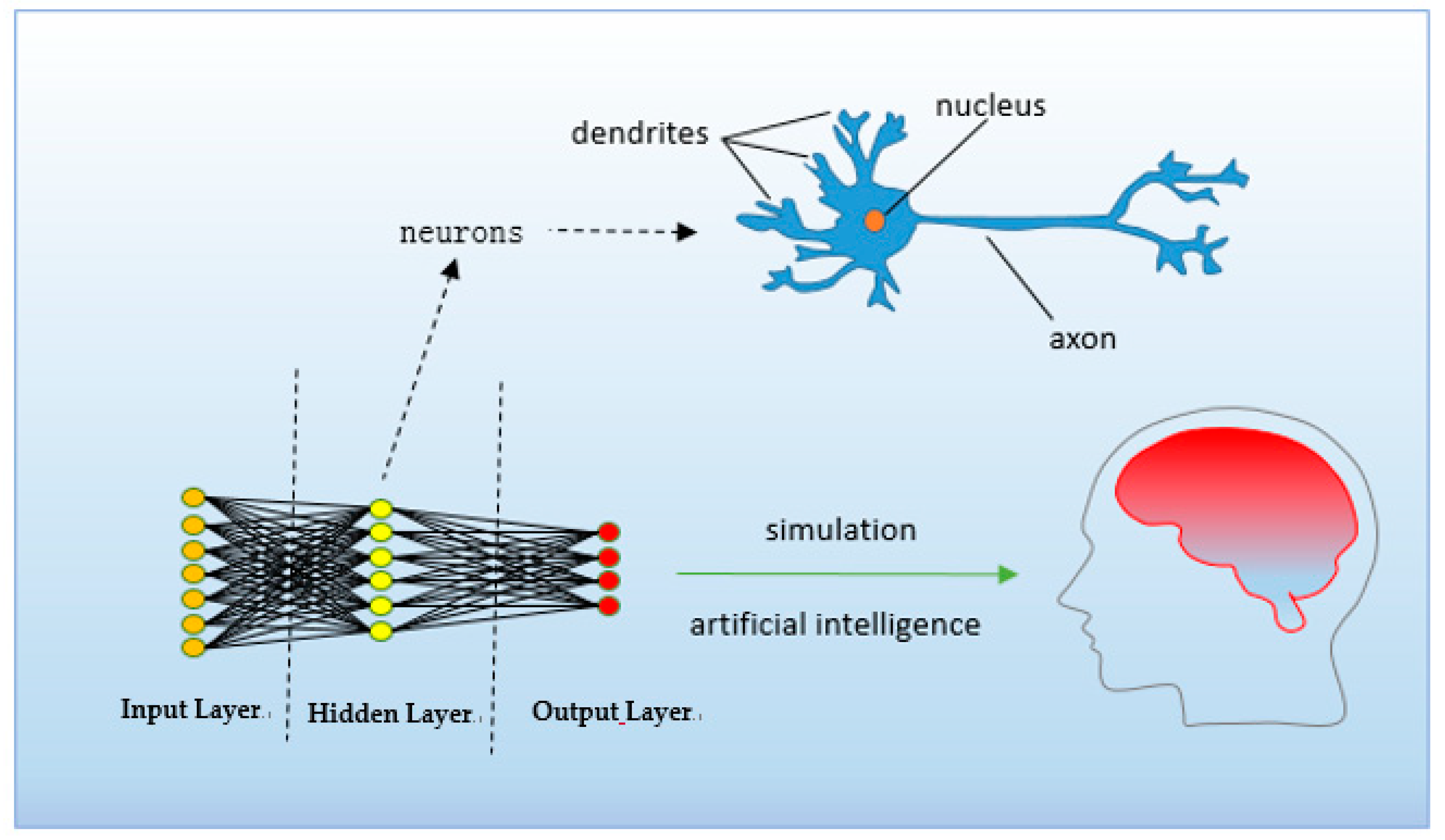
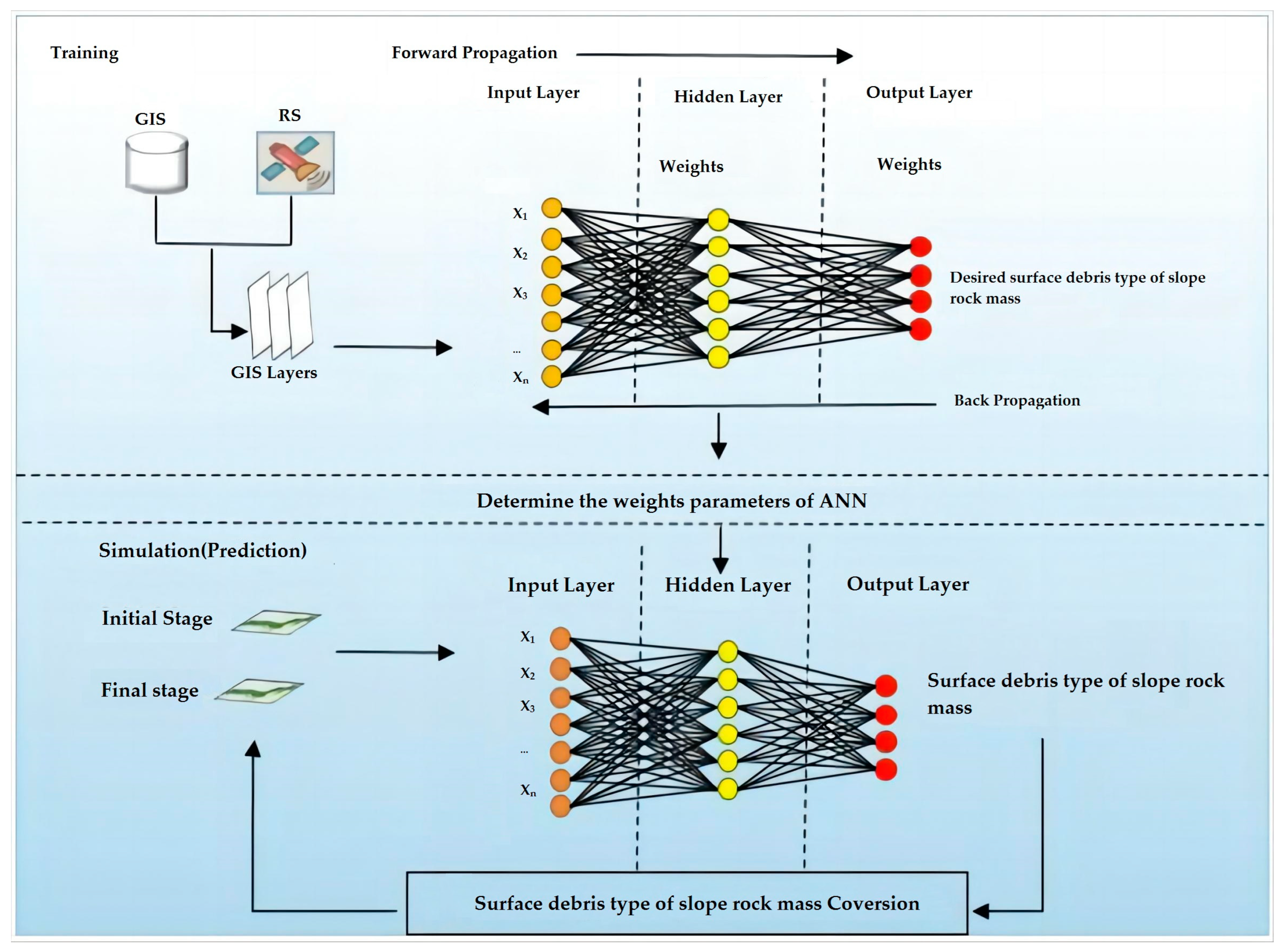
3.1. CA and ANN
3.2. Theoretical Basis
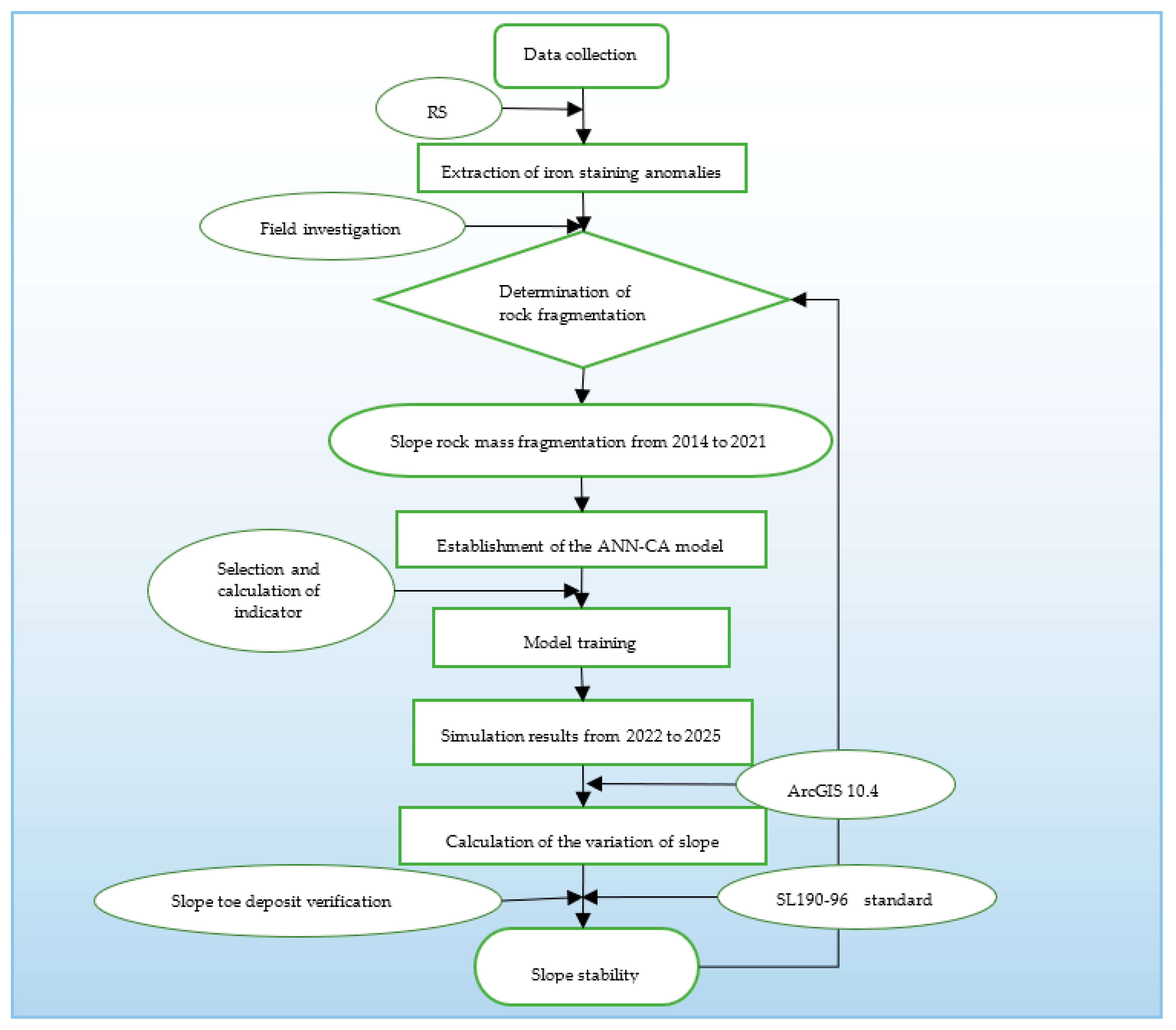
3.3. Model Implementation Process
4. Data Processing and Simulation
4.1. Image Acquisition and Preprocessing
4.2. Extraction of Iron Staining Abnormalities
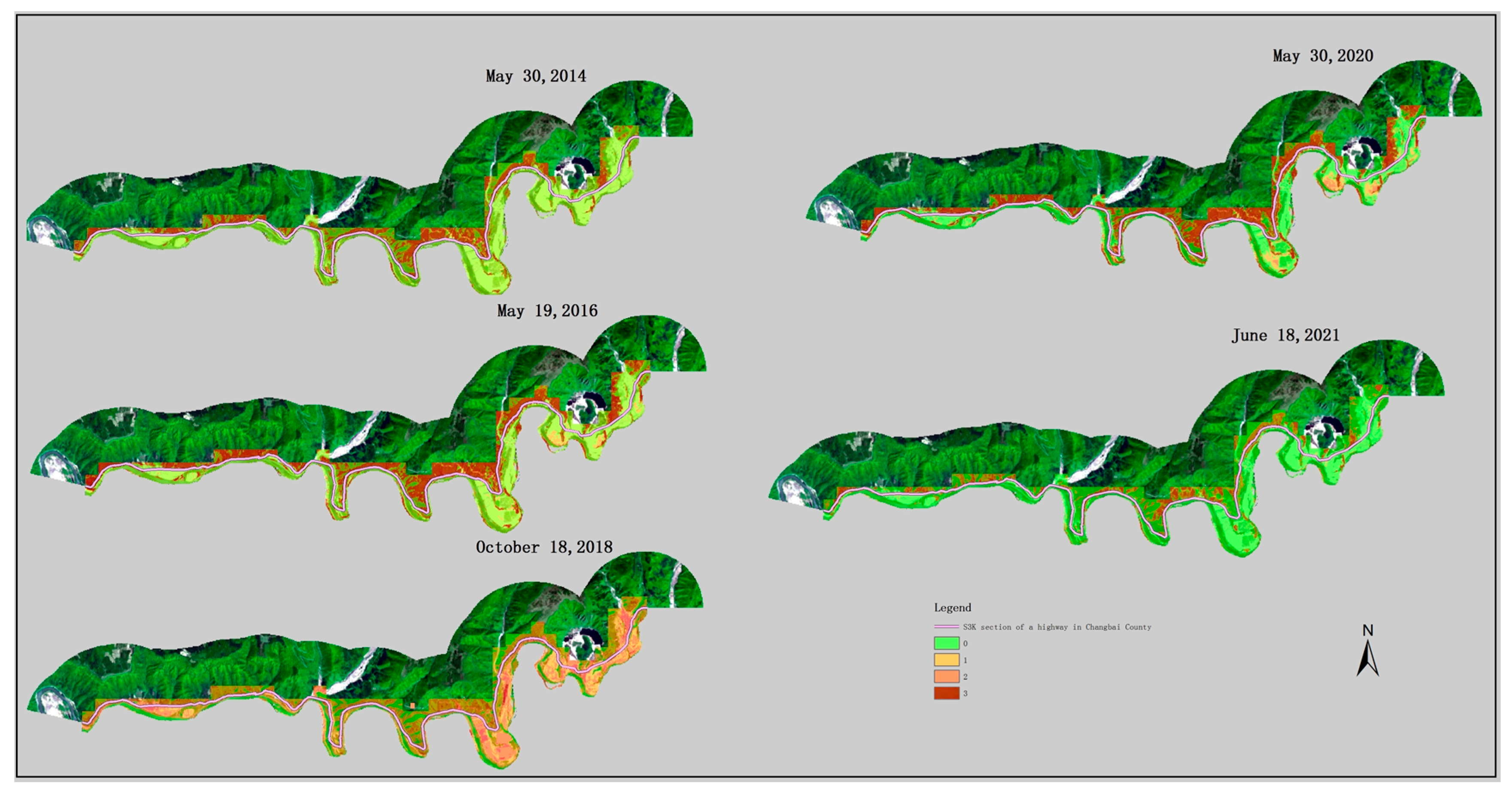
4.3. Fragmentation Classification of the Slope
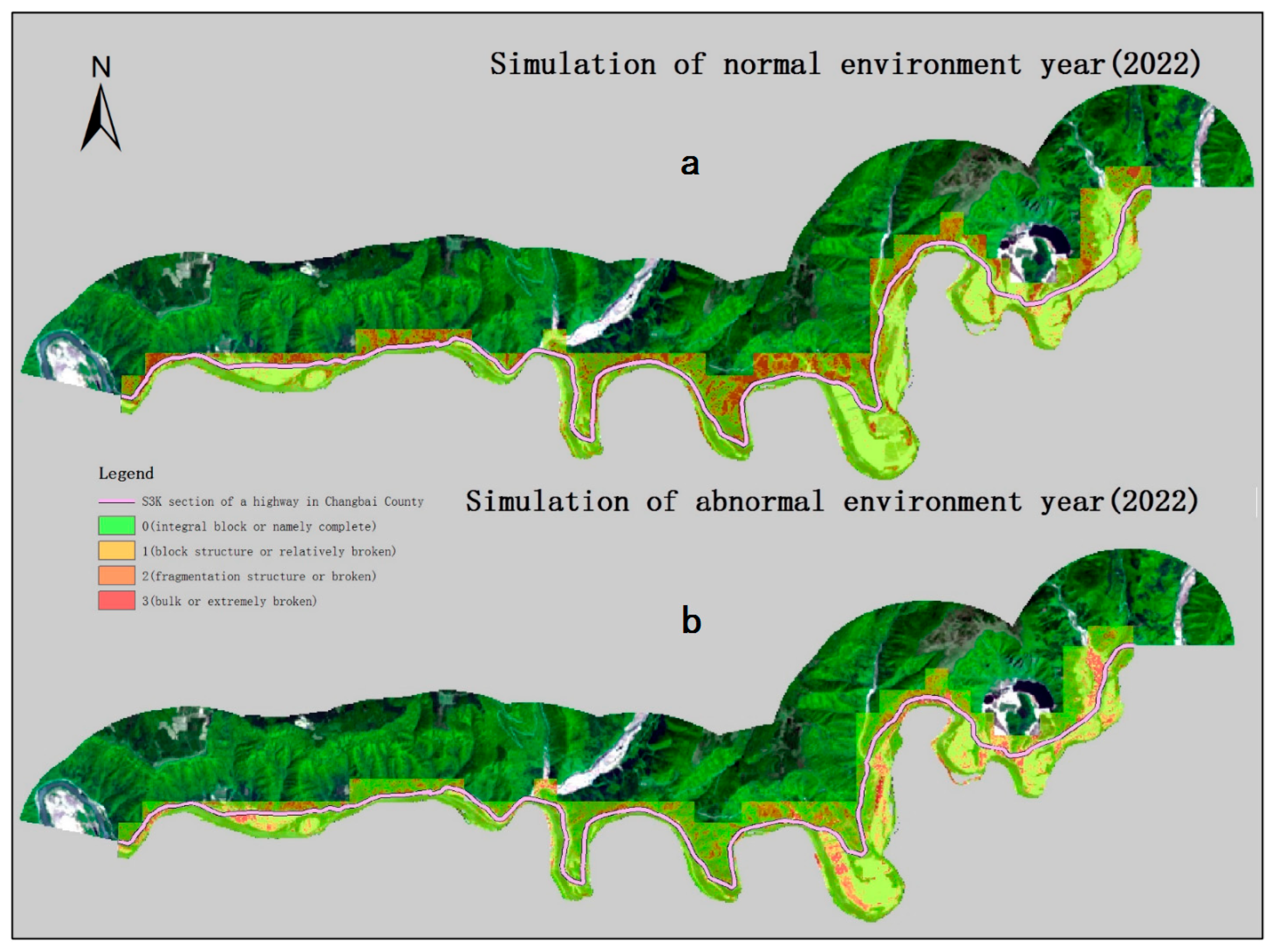
4.4. Simulation of Slope Instability Evolution
4.4.1. Indicator Selection and Acquisition
4.4.2. Model Training and Simulation
5. Analysis and Discussion
5.1. Analysis Process
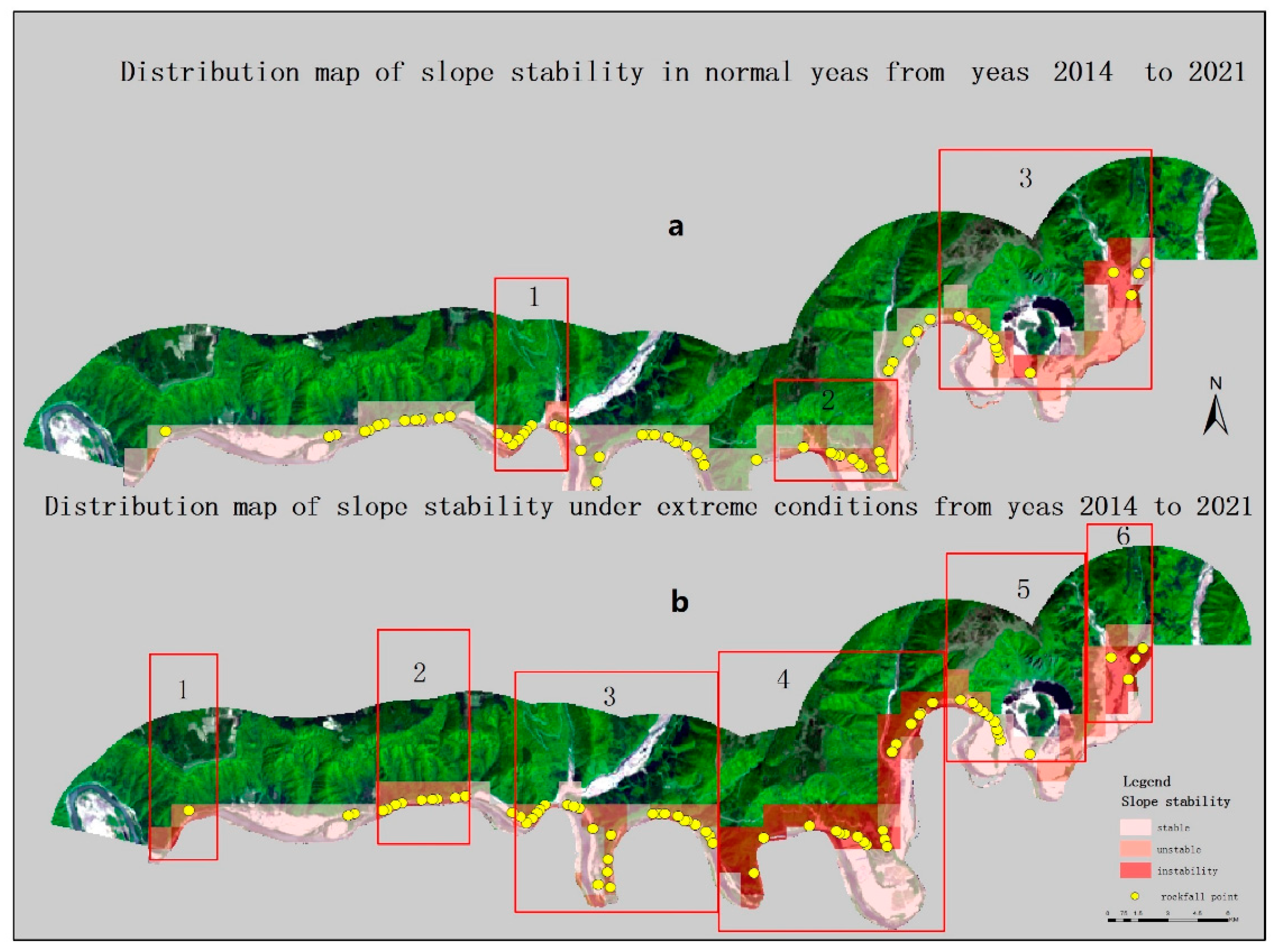
5.2. Field Investigation
5.3. Discussion
6. Conclusions
Author Contributions
Funding
Data Availability Statement
Acknowledgments
Conflicts of Interest
Appendix A

| No. | Microtopography | Slope Height (m) | Slope Width (m) | Slope Length (m) | Field Investigation of the Rock Mass Structure | Remote Sensing Analysis Results |
|---|---|---|---|---|---|---|
| 0 | Steep slope | 20 | 227 | 44 | Integral block | Bulk |
| 1 | Steep cliffs | 17 | 129 | 23 | Block structure | Block structure |
| 2 | Steep cliffs | 14 | 179 | 15 | Block structure | Block structure |
| 3 | Steep cliffs | 25 | 205 | 30 | Integral block | Integral block |
| 4 | Steep slope | 120 | 270 | 177 | Block structure | Block structure |
| 5 | Steep cliffs | 30 | 107 | 37 | Block structure | Block structure |
| 6 | Steep cliffs | 35 | 115 | 42 | Integral block | granular structure |
| 7 | Gentle slope | 7 | 245 | 10 | Integral block | granular structure |
| 8 | Steep slope | 15 | 97 | 21 | Block structure | Block structure |
| 9 | Steep slope | 12 | 151 | 18 | Block structure | Block structure |
| 10 | Steep slope | 12 | 21 | 14 | Fragmentation structure | Fragmentation structure |
| 11 | Steep cliffs | 19 | 256 | 29 | Block structure | Block structure |
| 12 | Steep slope | 12 | 212 | 17 | granular structure | granular structure |
| 13 | Steep cliffs | 14 | 171 | 17 | Block structure | Block structure |
| 14 | Steep slope | 16 | 235 | 25 | Block structure | Block structure |
| 15 | Steep slope | 8 | 94 | 14 | Block structure | Block structure |
| 16 | Steep cliffs | 44 | 151 | 50 | Block structure | Block structure |
| 17 | Steep slope | 15 | 17 | 17 | Integral block | granular structure |
| 18 | Steep slope | 6 | 169 | 8 | Block structure | Block structure |
| 19 | Steep slope | 8 | 351 | 10 | Block structure | Block structure |
| 20 | Steep slope | 18 | 56 | 26 | Block structure | Block structure |
| 21 | Steep slope | 7 | 40 | 10 | granular structure | granular structure |
| 22 | Steep cliffs | 17 | 79 | 20 | Integral block | Integral block |
| 23 | Steep slope | 24 | 100 | 31 | Block structure | Block structure |
| 24 | Steep slope | 18 | 151 | 22 | Block structure | Block structure |
| 25 | Steep slope | 22 | 130 | 31 | Block structure | Block structure |
| 26 | Steep slope | 33 | 99 | 38 | Block structure | Block structure |
| 27 | Steep slope | 14 | 233 | 23 | Fragmentation structure | Fragmentation structure |
| 28 | Steep slope | 35 | 258 | 40 | Integral block | granular structure |
| 29 | Steep slope | 11 | 169 | 19 | Block structure | Block structure |
| 30 | Steep slope | 19 | 74 | 22 | Block structure | Block structure |
| 31 | Steep slope | 16 | 52 | 22 | Block structure | Block structure |
| 32 | Steep cliffs | 7 | 252 | 6 | Integral block | granular structure |
| 33 | Steep cliffs | 11 | 79 | 13 | Block structure | Block structure |
| 34 | Steep cliffs | 21 | 89 | 24 | Block structure | Block structure |
| 35 | Steep cliffs | 19 | 203 | 31 | Block structure | Block structure |
| 36 | Steep slope | 27 | 52 | 35 | granular structure | granular structure |
| 37 | Steep slope | 6 | 10 | 7 | Integral block | Integral block |
| 38 | Steep slope | 4 | 172 | 5 | Integral block | Integral block |
| 39 | Steep slope | 5 | 151 | 7 | Fragmentation structure | Fragmentation structure |
| 40 | Steep slope | 4 | 73 | 5 | Block structure | Block structure |
| 41 | Steep slope | 7 | 176 | 11 | Block structure | Block structure |
| 42 | Gentle slope | 12 | 161 | 18 | Block structure | Block structure |
| 43 | Steep slope | 13 | 27 | 19 | Block structure | Block structure |
| 44 | Steep slope | 16 | 185 | 22 | Block structure | Block structure |
| 45 | Steep slope | 18 | 402 | 22 | Block structure | granular structure |
| 46 | Steep cliffs | 7 | 94 | 7 | Block structure | Block structure |
| 47 | Steep slope | 5 | 30 | 8 | granular structure | granular structure |
| 48 | Steep slope | 6 | 305 | 10 | Fragmentation structure | Fragmentation structure |
| 49 | Steep slope | 15 | 162 | 21 | Block structure | Block structure |
| 50 | Steep slope | 25 | 167 | 32 | Block structure | Block structure |
| 51 | Steep slope | 25 | 90 | 33 | Block structure | Block structure |
| 52 | Steep slope | 22 | 11 | 30 | Block structure | Block structure |
| 53 | Steep slope | 4 | 40 | 6 | Integral block | granular structure |
| 54 | Steep slope | 14 | 108 | 21 | Fragmentation structure | Fragmentation structure |
| 55 | Steep slope | 10 | 212 | 14 | Integral block | Integral block |
| 56 | Steep cliffs | 6 | 65 | 7 | Block structure | Block structure |
| 57 | Steep slope | 7 | 160 | 9 | Integral block | Integral block |
| 58 | Steep slope | 2 | 177 | 3 | Fragmentation structure | Fragmentation structure |
| 59 | Steep slope | 33 | 12 | 43 | Block structure | Block structure |
| 60 | Steep slope | 19 | 30 | 22 | Integral block | Integral block |
| 61 | Steep slope | 26 | 50 | 28 | Integral block | Integral block |
| 62 | Steep slope | 16 | 127 | 19 | Integral block | Integral block |
| 63 | Steep slope | 24 | 64 | 24 | Integral block | Integral block |
| 64 | Steep slope | 8 | 77 | 11 | Integral block | Integral block |
| 65 | Steep slope | 17 | 133 | 26 | granular structure | granular structure |
| 66 | Steep slope | 22 | 254 | 38 | Integral block | Integral block |
| 67 | Steep slope | 26 | 191 | 30 | Block structure | Block structure |
| 68 | Steep slope | 34 | 283 | 36 | Block structure | Block structure |
| 69 | Steep cliffs | 25 | 249 | 33 | Integral block | Integral block |
| 70 | Steep cliffs | 11 | 44 | 18 | Block structure | Block structure |
References
- Moon, G.-B.; You, Y.-M.; Yun, H.-S.; Suh, Y.-H.; Seo, Y.-S.; Baek, Y. Analysis of Magnitude and Behavior of Rockfall for Volcanic Rocks in Ulleung-Do. J. Eng. Geol. 2014, 24, 373–381. [Google Scholar] [CrossRef] [Green Version]
- Yan, X.; Xu, B.; Zhang, L.; Wang, W.; Yan, C. Mechanism analysis of a landslide in highly weathered volcanic rocks of Niushoushan Hill in Nanjing. Environ. Earth Sci. 2019, 78, 676. [Google Scholar] [CrossRef]
- Wijaya, I.P.K.; Zangel, C.; Straka, W.; Ottner, F. Geological Aspects of Landslides in Volcanic Rocks in a Geothermal Area (Kamojang Indonesia). In Advancing Culture of Living with Landslides; Springer: Cham, Switzerland, 2017; pp. 429–437. [Google Scholar] [CrossRef]
- Alexandre, P.; Cardoso, D.; Lopes, H. Stabilization of landslides in the Lisbon Volcanic Complex. International Congress on Rock Mechanics 2007. Available online: https://xueshu.baidu.com/usercenter/paper/show?paperid=1m5u0gn0a11y04e0by0m0v506d627463&site=xueshu_se (accessed on 8 June 2023).
- Gao, Y.; Li, B.; Gao, H.; Chen, L.; Wang, Y. Dynamic characteristics of high-elevation and long-runout landslides in the Emeishan basalt area: A case study of the Shuicheng “7.23” landslide in Guizhou, China. Landslides 2020, 17, 1663–1677. [Google Scholar] [CrossRef]
- Chen, Z.; Zhang, F.; Chang, J.; Lv, Y. Investigation on Characteristics of Large-Scale Creep Landslides. In Proceedings of the GeoShanghai 2018 International Conference: Geoenvironment and Geohazard, GSIC 2018, Shanghai, China, 27–30 May 2018; Farid, A., Chen, H., Eds.; Springer: Singapore, 2018. [Google Scholar] [CrossRef]
- Huang, Y.; Sun, Z.; Bao, C.; Huang, M.; Li, A.; Liu, M. A Typical Basalt Platform Landslide: Mechanism and Stability Prediction of Xiashan Landslide. Adv. Civ. Eng. 2021, 2021, 6697040. Available online: https://www.hindawi.com/journals/ace/2021/6697040/ (accessed on 8 June 2023). [CrossRef]
- Ngapouth, I.M.; Meli’I, J.L.; Gweth, M.M.A.; Pokam, B.P.G.; Koffi, Y.P.; Njock, M.C.; Nkoma, M.A.P.; Nouck, P.N. Analysis of safety factors for roads slopes in central Africa. Eng. Fail. Anal. 2022, 138, 106359. [Google Scholar] [CrossRef]
- Shen, S. Research on the Geological Environment and Slope Stalilitiy of Mountain Area in Sountheasten of Jinlin Pronvice. Ph.D. Thesis, Jilin University, Changchun, China, 2010. [Google Scholar]
- Zhou, R. The Slop Stability Analysis of Basalt Residual Soil in Guizhou. Master’s Thesis, Wuhan University of Science and Technology, Wuhan, China, 2013. Available online: http://www.doc88.com/p-9176759919137.html (accessed on 8 June 2023).
- Li, Y. Research on Strength Characteristics of Unsaturated Basalt Residual Soil and Its Slope Stability. Master’s Thesis, Wuhan University of Science and Technology, Wuhan, China, 2017. Available online: https://kns.cnki.net/kcms/detail/detail.aspx?dbcode=CMFD&dbname=CMFD202101&filename=1020105452.nh&uniplatform=NZKPT&v=A1_Lv5ABbWUXSQuf770uwBjx1APMO1icaRnx2VX4sZlvsjm4AvJukhDu6qQo6DLa (accessed on 8 June 2023).
- Kainthola, A.; Singh, P.; Singh, T. Stability investigation of road cut slope in basaltic rockmass, Mahabaleshwar, India. Geosci. Front. 2015, 6, 837–845. [Google Scholar] [CrossRef] [Green Version]
- He, X.F. Analysis and Study on the Stability of the Xinajian Village Slope in the Baihetan Hydropower Station. Master’s Thesis, North China University of Water Resources and Electric Power, Zhengzhou, China, 2018. Available online: https://kns.cnki.net/kcms/detail/detail.aspx?dbcode=CMFD&dbname=CMFD201802&filename=1018234911.nh&uniplatform=NZKPT&v=vv8HzK3Xi5G3W0WHQyd1BDMSZVu5oea5RZe8nJXw_P77toz3NdBP3tHW1k4ub9Jv (accessed on 8 June 2023).
- Liu, X.; Chen, X.; Su, M.; Zhang, S.; Lu, D. Stability Analysis of a Weathered-Basalt Soil Slope Using the Double Strength Reduction Method. Adv. Civ. Eng. 2021, 2021, 6640698. [Google Scholar] [CrossRef]
- Zhang, Y. Study on Influencing Factors of Basalt-Mudston Slope Stability and Envolution Mechanism of Rainfall Landslide. Master’s Thesis, Inner Mongolia University of Technology, Hohhot, China, 2021. Available online: https://d.wanfangdata.com.cn/thesis/D02512376 (accessed on 8 June 2023).
- Wang, X.; Liu, H.; Sun, J. A New Approach for Identification of Potential Rockfall Source Areas Controlled by Rock Mass Strength at a Regional Scale. Remote Sens. 2021, 13, 938. [Google Scholar] [CrossRef]
- Mazzanti, P.; Schilirò, L.; Martino, S.; Antonielli, B.; Brizi, E.; Brunetti, A.; Margottini, C.; Mugnozza, G.S. The Contribution of Terrestrial Laser Scanning to the Analysis of Cliff Slope Stability in Sugano (Central Italy). Remote Sens. 2018, 10, 1475. [Google Scholar] [CrossRef] [Green Version]
- Xu, Q.; Ye, Z.; Liu, Q.; Dong, X.; Li, W.; Fang, S.; Guo, C. 3D Rock Structure Digital Characterization Using Airborne LiDAR and Unmanned Aerial Vehicle Techniques for Stability Analysis of a Blocky Rock Mass Slope. Remote Sens. 2022, 14, 3044. [Google Scholar] [CrossRef]
- Nath, S.K.; Sengupta, A.; Srivastava, A. Remote sensing GIS-based landslide susceptibility & risk modeling in Darjeeling–Sikkim Himalaya together with FEM-based slope stability analysis of the terrain. Nat. Hazards 2021, 108, 3271–3304. [Google Scholar] [CrossRef]
- Omar, H. Slope Stability Using Remote Sensing and Geographic Information System Along Karak Highway, Malaysia. Master’s Thesis, Universiti Teknologi Malaysia, Johor Bahru, Malaysia, 2010. Available online: https://core.ac.uk/display/11791805 (accessed on 8 June 2023).
- Wang, S. Study on Stability of Cataclastic High Slope of Reservoir Bank Highway; Beijing University of Technology Press: Beijing, China, 2016; pp. 5–35. [Google Scholar]
- Chen, Z.Q.; Wang, L.Z.; Kong, H.L.; Ni, X.Y.; Yao, B.H. A method for calculating permeability parameters of variable mass of broken rock. Chin. J. Appl. Mech. 2014, 31, 927–932. Available online: http://www.cnki.com.cn/Article/CJFDTotal-YYLX201406019.htm (accessed on 8 June 2023).
- Wang, Q.; Chen, J.P. Extraction and grading of remote sensing alteration anomaly based on the fractal theory. Geol. Bull. China 2009, 28, 285–288. Available online: https://d.wanfangdata.com.cn/periodical/zgqydz200902022 (accessed on 8 June 2023).
- Wei, W.; Shen, J.; Miao, Z.; Liu, H.; Li, G.; Nie, D. Influence Analysis of Weathering and Altering for Physical and Mechanical Characteristics of Granite Porphyry. J. Eng. Geol. 2012, 20, 599–605. Available online: http://www.cnki.com.cn/Article/CJFDTotal-GCDZ201204018.htm (accessed on 8 June 2023).
- Yang, G.-L. Altered-Rock Characteristics and Its Engineering Respondences Studing—Exemplified by Xiaowan Hydroppower Station Lancang River. Ph.D. Thesis, Chengdu University of Technology, Chengdu, China, 2007. Available online: https://www.doc88.com/p-6079867752006.html (accessed on 8 June 2023).
- Miao, Z.; Shen, J.F.; Li, W.G.; Li, J.B.; Chen, W.D. Alteration and geological characteristics of granite in dam area of Dagangshan Hydropower Station. Yangtze River 2013, 44, 23–25. Available online: https://wenku.baidu.com/view/4ab31c0627284b73f3425010.html (accessed on 8 June 2023).
- Weng, H.-J.; Kong, F.-Q.; Wei, L.-M.; Lu, Y.; Sun, N. Elements migration of gold mineralization and wall-rock alteration process in Baguamiao. J. Guilin Univ. Technol. 2015, 35, 721–726. Available online: https://www.cnki.com.cn/Article/CJFDTotal-GLGX201504009.htm (accessed on 8 June 2023).
- Qian, X. On the Development of Geo-Science. Acta Geogr. Sin. 1989, 44, 257–261. Available online: https://max.book118.com/html/2017/0727/124569366.shtm (accessed on 8 June 2023).
- Jin, M.; Wang, H.; Zhang, W.; Wang, X. Method for extraction of ferric contamination anomaly from high—Resolution remote sensing data and its applications. Remote Sens. Land Resour. 2015, 27, 122–127. Available online: https://max.book118.com/html/2017/0911/133298029.shtm (accessed on 8 June 2023).
- Liu, J.-Q.; Chen, S.-S.; Guo, Z.-F.; Guo, W.-F.; He, H.-Y.; You, H.-T.; Kim, H.-M.; Sung, G.-H.; Kim, H. Geological background and geodynamic mechanism of Mt. Changbai volcanoes on the China–Korea border. Lithos 2015, 236–237, 46–73. [Google Scholar] [CrossRef]
- Wei, H. TianChi Volcano, Changbaishan; Seismological Press: Beijing, China, 2014; pp. 158–253. [Google Scholar]
- Zhang, L.; Li, G.-J. Analysis on stability of slope in Tianchi Lake area of Changbaishan Mountain. Glob. Geol. 2005, 24, 378–381. Available online: https://www.docin.com/p-854189838.html (accessed on 8 June 2023).
- Wang, Y. Stability Analysis and Control Engineering of Landslide in S3k Section of Yangjiang Highway in Changbai County, Jilin. Master’s Thesis, Jilin University, Changchun, China, 2017. Available online: http://cdmd.cnki.com.cn/Article/CDMD-10183-1018000028.htm (accessed on 8 June 2023).
- Ni, X.; Nan, Y. Comprehensive assessment of geological disasters risk in Changbai Mountain region based on GIS. J. Nat. Disasters 2014, 23, 112–120. Available online: http://www.dlyj.ac.cn/CN/Y2014/V33/I7/1348 (accessed on 8 June 2023).
- Wang, H.; Cao, B.-L. Research on influence factors of collapse-slide in tourist area of Changbai Mountain. Glob. Geol. 2004, 23, 56–59. Available online: https://d.wanfangdata.com.cn/periodical/sjdz200401010 (accessed on 8 June 2023).
- Qian, L.; Zang, S. Differentiation Rule and Driving Mechanisms of Collapse Disasters in Changbai County. Sustainability 2022, 14, 2074. [Google Scholar] [CrossRef]
- Liu, Z.; Zhang, Y.; Ishikawa, Y.; Nakamura, H. Landslide Hazard and Risk Assessment on the Northern Slope of Mt. Changbai, China. Acta Geol. Sin. 2008, 82, 214–224. [Google Scholar] [CrossRef]
- Li, X.; Ye, J.; Liu, X.; Yang, Q. Geographic Simulation System: Cellular Automata and Multi-Agent; Science Press: Beijing, China, 2007. [Google Scholar]
- Chopard, B.; Droz, M. Cellular Automata Simulation of Physical Systems; Tsinghua University Press: Beijing, China, 2003; pp. 1–2. [Google Scholar]
- Zhou, C.H.; Sun, Z.L.; Xie, Y.C. Geo-Celluar Automata Research; Science Press: Beijing, China, 1999. [Google Scholar]
- Carson, M.A.; Kirkby, M.J. Hill Slope Form and Process; Science Press: Beijing, China, 1984. [Google Scholar]
- Davis, W.M. The geographical cycle. Geogr. J. 1899, 14, 481–504. [Google Scholar] [CrossRef]
- Hunt, G.R. Spectral signatures of particulate minerals in the visible and near infrared. Geophysics 1977, 42, 501–513. [Google Scholar] [CrossRef] [Green Version]
- Zhang, Y.; Yang, J.; Chen, W. A Study of the Method for Extractioh of Alteration Anomales from the ETM+ (TM) Data and Its Application: Geologic Basis and Spectral Precondition. Remote Sens. Land Resour. 2002, 4, 30–36. Available online: https://www.doc88.com/p-2942807720195.html (accessed on 8 June 2023).
- Zhang, C.; Nan, W.; Tai, S.; Li, J. Analysis of meterological conditions of TianChi in Changbai Mountain. J. Agric. Sci. Yanbian Univ. 2007, 29, 33–36. Available online: http://qikan.cqvip.com/Qikan/Article/Detail?id=24058611 (accessed on 8 June 2023).
- Qian, L.; Zang, S. Research on the Developing Zone of Collapse and Landslide or Debris Flow Geohazards Based on Grid-GIS and Grey Correlation Model. Geomat. World 2020, 27, 64–74. Available online: http://www.cnki.com.cn/Article/CJFDTotal-CHRK202006010.htm (accessed on 8 June 2023).
- Du, T. The Comparison among Fusion Algorithms of Landsat8 OLI Remote-Sensing Imagery and the Analysis on Adaptability of the Classification of Land Use. Master’s Thesis, Northwest University, Xi’an, China, 2015. Available online: https://cdmd.cnki.com.cn/Article/CDMD-10697-1015326821.htm (accessed on 8 June 2023).
- Zhao, J.; Ma, Y.; Shi, Y.; Hao, S.; Ma, X. Prediction of soil erosion evolution in counties in the loess hilly region based on ANN-CA model. Sci. Soil Water Conserv. 2021, 19, 60–68. [Google Scholar] [CrossRef]
- Zhang, F.; Tang, G.A.; Cao, M.; Yang, J.Y. Simulation of Positive and Negative Terra in Evolution in Small Loess Watershed Based oil ANN—CA Model. Geogr. Geo-Inf. Sci. 2013, 29, 28–31. Available online: http://www.doc88.com/p-9019460823176.html (accessed on 8 June 2023).
- Littidej, P.; Uttha, T.; Pumhirunroj, B. Spatial Predictive Modeling of the Burning of Sugarcane Plots in Northeast Thailand with Selection of Factor Sets Using a GWR Model and Machine Learning Based on an ANN-CA. Symmetry 2022, 14, 1989. [Google Scholar] [CrossRef]
- Li, X.; Yeh, A.G.O. Neural-network-based cellular automata for simulating multiple land use changes using GIS. Int. J. Geogr. Inf. Sci. 2002, 16, 323–343. [Google Scholar] [CrossRef]
- Bell, D.H. High intensity rainstorms and geological hazaeds: Cyclone Alison, March 1975, Kaikoura, New Zealand. Bull. Int. Assoc. Eng. Geol. 1976, 13, 189–200. [Google Scholar] [CrossRef]
- Liu, F.; Tao, F.; Xiao, D.; Zhang, S.; Wang, M.; Zhang, H.; Bai, H. The contributions of leaf area index and precipitation to surface energy balance in the process of land cover change. Geogr. Res. 2014, 33, 1264–1274. Available online: http://www.dlyj.ac.cn/CN/10.11821/dlyj201407007 (accessed on 8 June 2023).
- Zhang, W.; Wang, J.; Sun, L.; Wang, Y. Disaster System and Disaster Dynamics; Science Press: Beijing, China, 2011; pp. 77–90. [Google Scholar]
- Zhao, H.; Wu, Q.; Liu, X.; Wang, Y.; Han, B. A Preliminary Study on the Exchange Approches of Substance and Energy in the Soil and Water Loss Systems. J. Soil Water Conserv. 1993, 7, 61–68. Available online: https://www.doc88.com/p-996568863441.html?r=1 (accessed on 8 June 2023).
- Yang, S.; Wang, Z.; Zhao, C.; Cai, M. Remote Sensing Hydrological Digital Experiment—EcoHAT User Manual; Science Press: Beijing, China, 2015; pp. 57–60. [Google Scholar]
- Zeng, H.; Guo, Q.-H.; Yu, H. Spatial analysis of artificial landscape transform in FengGang town, DongGuan city. Acta Ecol. Sin. 1999, 19, 298–303. [Google Scholar] [CrossRef]
- Shi, D.; Shi, X.; Li, D.; Liang, Y. Study on dynamic monitoring of soil erosion using remote sensing technique. Acta Pedol. Sin. 1996, 33, 48–58. Available online: http://www.cnki.com.cn/Article/CJFDTotal-TRXB601.005.htm (accessed on 8 June 2023).
- Shang, Y.; Li, K.; Wang, K. Insights of Innovation and Development of Rock Mass Structure Dynamic Controlling Froconstruction-Triggered Geohazard. Chin. J. Rock Mech. Eng. 2013, 32, 1129–1136. Available online: http://www.cqvip.com/QK/96026X/201306/46252635.html (accessed on 8 June 2023).
- Qiu, S.; Cao, L.; Yang, W. Dynamic monitoring of land use change through RS in the upper Minjiang river. Comput. Tech. Geophys. Geochem. Explor. 2021, 43, 390–396. Available online: http://qikan.cqvip.com/Qikan/Article/Detail?id=7104675597 (accessed on 8 June 2023).
- LI, X.; Fang, J.; Piao, S. Landuse Changes and Its Implication to the Ecological Consequences in Lower Yangtze Region. Acta Geogr. Sin. 2003, 58, 559–667. Available online: https://www.docin.com/p-190146069.html (accessed on 8 June 2023).
- Li, M.; Wang, J.; Wu, P. Dynamic Change and Driving Factors Analysis of Shihezi Land Use Based on Remote Sensing. Anhui Agric. Sci. Bull. 2021, 27, 110–116. Available online: http://cstj.cqvip.com/Qikan/Article/Detail?id=7104389930 (accessed on 8 June 2023).
- Zhang, X.; Liu, N.; Zhao, Y.; Zhang, Y.; Ma, F.; Wu, D.; Liu, H. Spatial and Temporal Variability Characteristics and Prediction of Land Use in Yinchuan from 2000 to 2020. Sci. Technol. Eng. 2021, 21, 10156–10164. Available online: http://stae.com.cn/jsygc/article/abstract/2102062 (accessed on 8 June 2023).
- Wang, X.; Bao, Y. Study on the methods of land use dynamic change research. Prog. Geogr. 1999, 18, 81–87. Available online: https://wenku.baidu.com/view/37c5762815fc700abb68a98271fe910ef02dae7b.html (accessed on 8 June 2023).


| Date | PC | Band 2 | Band 4 | Band 5 | Band 6 | Contribution Rate (%) |
|---|---|---|---|---|---|---|
| 19 May 2016 | PC1 | 0.094610 | −0.098194 | 0.989432 | 0.049301 | 76.49 |
| PC2 | −0.617834 | −0.773717 | −0.010745 | −0.139745 | 22.33 | |
| PC3 | −0.646450 | 0.398389 | 0.069112 | 0.647002 | 0.94 | |
| PC4 | 0.437531 | −0.482707 | −0.127011 | 0.747950 | 0.24 | |
| 30 May 2020 | PC1 | 0.195103 | −0.033706 | 0.978984 | 0.048875 | 77.42 |
| PC2 | 0.674310 | 0.720196 | −0.115350 | 0.115408 | 21.45 | |
| PC3 | 0.646498 | −0.540702 | −0.121278 | −0.524379 | 0.86 | |
| PC4 | 0.298801 | −0.433386 | −0.116516 | 0.842211 | 0.27 |
| No. | Longitude and Latitude of the Center of the Survey Area | Investigation of the Slope Rock Mass | DN Value Range |
|---|---|---|---|
| 1 | 127°55′45′′, 41°27′27′′ | Broken to extremely broken | 224~255 |
| 2 | 127°50′46′′, 41°25′11′′ | Strongly weathered to weakly weathered, and relatively broken | 202~255 |
| 3 | 127°48′05′′, 41°25′18′′ | Strongly weathered to weakly weathered, and relatively broken | 190~255 |
| 4 | 127°46′53′′, 41°25′23′′ | Completely weathered to strongly weathered, and broken to extremely broken | 196~255 |
| 5 | 127°40′33′′, 41°25′12′′ | Strongly weathered to weakly weathered, and relatively broken | 200~255 |
| 6 | ---- | Weakly weathered, and relatively complete | 88~255 |
| 7 | ---- | Relatively broken | 187~255 |
| 8 | ---- | Relatively complete | 90~255 |
| 9 | ---- | Extremely broken | 242~255 |
| 10 | ---- | Broken | 197~255 |
| No. | Control Factor | Acquisition Method | Original Data Value Range | Standardization Scope |
|---|---|---|---|---|
| 1 | Annual rainfall | IDW | 622–699 mm | 0~1 |
| 2 | Monthly extreme rainfall | IDW | >200 mm | 0–1 |
| 3 | Slope | Slope tool in ArcGIS10.4 software | 0~81.28° | 0~1 |
| 4 | Topographic relief | Max-min | 0~80 | 0~1 |
| 5 | Surface roughness | Equation (5) | 1–6.15 | 0–1 |
| 6 | LAI | Equation (6) | −6.9–14.4 | 0–1 |
| 7 | NDVI | Equation (7) | −1–1 | 0–1 |
| 8 | Rd | Equation (8) | 0–70 | 0–1 |
| 9 | DT | Equation (9) | 0.83~0.9 | 0~1 |
| Time | Abnormal Change Area of Iron Staining Anomalies (km2) | Ratio of Iron Staining Abnormalities Indicating Change to the Grid Area | Corresponding Historical Disaster Points (Number of Places) | Stability Assessment | Spatial Location |
|---|---|---|---|---|---|
| Normal year change information (From 2014 to 2021) | 0.4600 | <10% | 38 | Stable | See Figure 8a |
| 1.2100 | 10–30% | 29 | Unstable | ||
| 1.9500 | >30% | 4 | Instability | ||
| Abnormal year change information (From 2014 to 2021) | 0.0700 | <10% | 0 | Stable | See Figure 8b |
| 0.9500 | 10–30% | 8 | Unstable | ||
| 8.9100 | >30% | 63 | Instability | ||
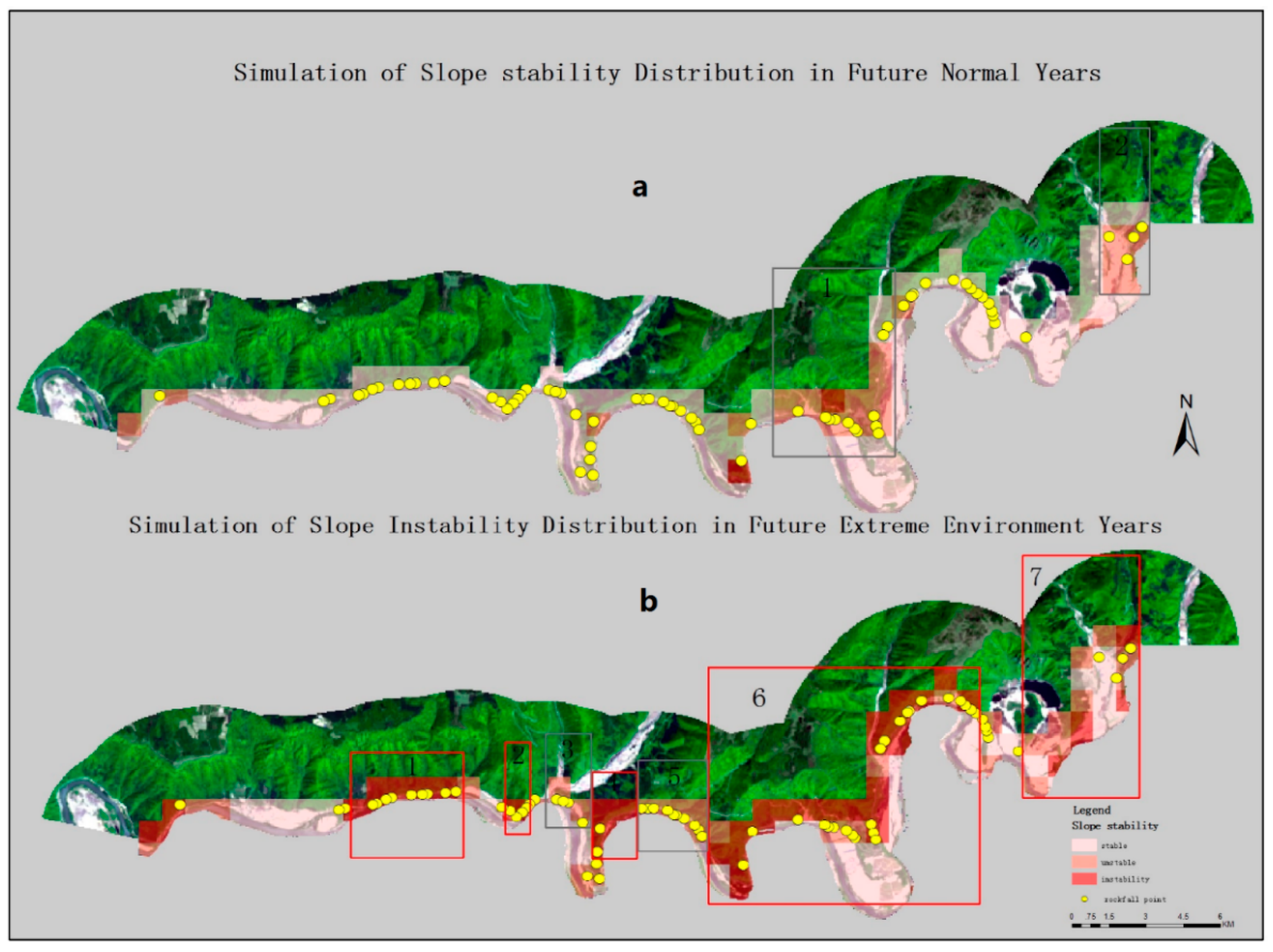
| Simulation of normal year change information (From 2022 to 2025) | 0.0046 | <10% | -- | Stable | See Figure 9a |
| 0.0107 | 10–30% | -- | Unstable | ||
| 0.0045 | >30% | -- | Instability | ||
| Simulation of abnormal year change information (From 2022 to 2025) | 0.0360 | <10% | -- | Stable | See Figure 9b |
| 1.3080 | 10–30% | -- | Unstable | ||
| 3.5230 | >30% | -- | Instability |
| Field Investigation No. | Zone ID | Field-Measured Data of Slope Rock and Soil Mass (Unit: m) | Volume of Slope Toe Deposits (m3) | ITRYC | ||||||
|---|---|---|---|---|---|---|---|---|---|---|
| Slope Top Elevation (m) | Footing Elevation (m) | Slope Length (m) | Slope Width | Slope Height (m) | Depth of Completely Weathered Zone (m) | Unloading Crack Depth (m) | ||||
| 1 | 1 | 582.60 | 561.60 | 31.00 | 130.00 | 22.00 | 1.20 | 0.00 | 2.60 | 0.887 |
| 2 | 2 | 555.60 | 530.60 | 33.00 | 249.00 | 25.00 | 1.10 | 0.60 | 10.00 | 0.951 |
| 3 | 558.50 | 541.00 | 17.50 | 44.00 | 11.00 | 0.00 | 0.00 | 12.00 | 0.951 | |
| 4 | 579.40 | 545.40 | 36.00 | 283.00 | 34.00 | 1.80 | 0.00 | 2.00 | 0.774 | |
| 5 | 560.20 | 534.20 | 30.00 | 191.00 | 26.00 | 0.80 | 0.60 | 1.50 | 0.737 | |
| 6 | 577.30 | 539.30 | 38.00 | 254.00 | 22.00 | 1.20 | 0.00 | 1.40 | 0.737 | |
| 7 | 568.80 | 548.30 | 24.00 | 89.00 | 20.50 | 1.60 | 0.00 | 2.34 | 0.991 | |
| 8 | 565.30 | 554.30 | 13.00 | 79.00 | 11.00 | 1.50 | 0.80 | 1.50 | 0.991 | |
| 9 | 564.20 | 547.20 | 20.00 | 79.00 | 17.00 | 1.20 | 0.00 | 4.50 | 0.903 | |
| 10 | 550.40 | 543.40 | 6.00 | 252.00 | 7.00 | 0.00 | 0.00 | 5.10 | 0.903 | |
| 11 | 3 | 574.90 | 573.10 | 3.00 | 177.00 | 1.80 | 1.60 | 0.00 | 3.75 | 0.490 |
| 12 | 600.30 | 589.30 | 19.00 | 169.00 | 11.00 | 0.00 | 0.00 | 7.00 | 0.921 | |
| 13 | 581.60 | 567.60 | 9.00 | 160.00 | 6.50 | 0.00 | 0.00 | 3.00 | 0.551 | |
| 14 | 582.00 | 574.00 | 10.00 | 351.00 | 8.00 | 1.60 | 0.00 | 3.15 | 0.551 | |
| 15 | 585.60 | 552.60 | 43.00 | 12.00 | 33.00 | 0.00 | 0.00 | 2.20 | 0.374 | |
| 16 | 557.20 | 551.20 | 7.00 | 65.00 | 6.00 | 0.00 | 0.00 | 18.75 | 0.909 | |
| 17 | 587.50 | 571.50 | 25.00 | 235.00 | 16.00 | 1.20 | 0.00 | 3.63 | 0.372 | |
| 18 | 578.90 | 568.90 | 14.00 | 212.00 | 10.00 | 0.80 | 0.00 | 1.20 | 0.372 | |
| 19 | 592.10 | 573.10 | 31.00 | 203.00 | 19.00 | 1.20 | 0.00 | 3.60 | 0.372 | |
| 20 | 563.40 | 556.00 | 10.00 | 40.00 | 7.40 | 1.80 | 0.00 | 3.00 | 0.281 | |
| 21 | 570.30 | 553.20 | 26.00 | 133.00 | 17.00 | 1.10 | 0.80 | 3.75 | 0.541 | |
| 22 | 556.00 | 548.00 | 11.00 | 77.00 | 8.00 | 1.00 | 0.70 | 3.15 | 0.541 | |
| 23 | 570.80 | 546.80 | 24.00 | 64.00 | 24.00 | 1.10 | 0.70 | 1.20 | 0.541 | |
| 24 | 569.10 | 543.10 | 28.00 | 50.00 | 26.00 | 0.80 | 0.00 | 8.00 | 0.569 | |
| 25 | 558.00 | 542.00 | 19.00 | 127.00 | 16.00 | 0.80 | 0.00 | 2.64 | 0.569 | |
| 26 | 567.40 | 548.40 | 22.00 | 30.00 | 19.00 | 2.00 | 0.70 | 3.00 | 0.569 | |
| 27 | 563.40 | 545.40 | 26.00 | 56.00 | 18.00 | 1.80 | 0.00 | 9.00 | 0.383 | |
| 28 | 568.70 | 546.70 | 22.00 | 74.00 | 19.00 | 0.80 | 0.00 | 3.00 | 0.383 | |
| 29 | 567.00 | 561.00 | 8.00 | 169.00 | 6.00 | 0.80 | 0.00 | 9.00 | 0.884 | |
| 30 | 575.40 | 560.40 | 17.00 | 17.00 | 15.00 | 0.80 | 0.00 | 1.00 | 0.884 | |
| 31 | 595.10 | 560.10 | 40.00 | 258.00 | 35.00 | 0.80 | 0.00 | 2.00 | 0.884 | |
| 32 | 594.90 | 651.90 | 38.00 | 99.00 | 33.00 | 0.80 | 0.00 | 1.20 | 0.581 | |
| 33 | 606.00 | 562.00 | 50.00 | 151.00 | 44.00 | 1.50 | 1.10 | 1.88 | 0.581 | |
| 34 | 569.90 | 561.90 | 14.00 | 94.00 | 8.00 | 1.50 | 0.80 | 3.00 | 0.696 | |
| 35 | 4 | 581.60 | 567.60 | 17.00 | 171.00 | 14.00 | 0.60 | 0.30 | 5.25 | 0.797 |
| 36 | 597.70 | 583.70 | 21.00 | 108.00 | 14.00 | 1.10 | 0.70 | 1.12 | 0.400 | |
| 37 | 587.10 | 568.10 | 29.00 | 256.00 | 19.00 | 1.00 | 0.80 | 6.00 | 0.800 | |
| 38 | 588.00 | 576.00 | 14.00 | 21.00 | 12.00 | 1.00 | 0.80 | 2.66 | 0.800 | |
| 39 | 587.10 | 583.10 | 6.00 | 40.00 | 4.00 | 1.00 | 0.70 | 15.00 | 0.800 | |
| 40 | 592.60 | 580.60 | 18.00 | 151.00 | 12.00 | 1.50 | 0.80 | 5.25 | 0.800 | |
| 41 | 612.40 | 597.40 | 21.00 | 97.00 | 15.00 | 1.00 | 0.80 | 9.00 | 0.800 | |
| 42 | 617.60 | 595.60 | 30.00 | 11.00 | 22.00 | 1.50 | 1.10 | 0.45 | 0.800 | |
| 43 | 649.70 | 634.70 | 21.00 | 162.00 | 15.00 | 0.00 | 0.00 | 9.75 | 0.800 | |
| 44 | 660.90 | 635.90 | 32.00 | 167.00 | 25.00 | 0.80 | 0.00 | 1.08 | 0.800 | |
| 45 | 669.50 | 644.50 | 33.00 | 90.00 | 25.00 | 0.80 | 0.00 | 2.25 | 0.800 | |
| 46 | 589.60 | 577.60 | 17.00 | 212.00 | 12.00 | 0.80 | 0.00 | 12.00 | 0.758 | |
| 47 | 633.50 | 627.00 | 8.00 | 102.00 | 6.50 | 1.20 | 0.80 | 3.63 | 0.450 | |
| 48 | 616.00 | 610.00 | 10.00 | 305.00 | 6.00 | 0.80 | 0.60 | 3.00 | 0.450 | |
| 49 | 626.50 | 620.00 | 7.00 | 94.00 | 6.50 | 1.20 | 0.80 | 1.20 | 0.544 | |
| 50 | 641.00 | 634.00 | 10.00 | 245.00 | 7.00 | 1.10 | 0.70 | 3.60 | 0.544 | |
| 51 | 665.00 | 630.00 | 42.00 | 115.00 | 35.00 | 0.00 | 0.00 | 1.88 | 0.709 | |
| 52 | 478.40 | 460.40 | 22.00 | 402.00 | 18.00 | 1.20 | 0.00 | 3.00 | 0.673 | |
| 53 | 5 | 643.60 | 627.60 | 22.00 | 185.00 | 16.00 | 0.80 | 0.00 | 15.00 | 0.122 |
| 54 | 695.70 | 665.70 | 37.00 | 107.00 | 30.00 | 0.00 | 0.00 | 1.10 | 0.855 | |
| 55 | 780.10 | 660.10 | 177.00 | 270.00 | 120.00 | 1.20 | 0.00 | 5.25 | 0.579 | |
| 56 | 651.00 | 626.00 | 30.00 | 205.00 | 25.00 | 0.20 | 0.30 | 0.90 | 0.579 | |
| 57 | 640.20 | 626.70 | 15.00 | 179.00 | 13.50 | 1.20 | 0.00 | 1.50 | 0.579 | |
| 58 | 6 | 649.50 | 645.00 | 7.00 | 151.00 | 4.50 | 1.20 | 0.00 | 1.12 | 0.800 |
| 59 | 648.90 | 623.00 | 35.00 | 52.00 | 27.00 | 1.20 | 0.00 | 6.00 | 0.800 | |
| 60 | 624.50 | 619.00 | 7.00 | 10.00 | 5.50 | 1.20 | 0.00 | 2.66 | 0.800 | |
| 61 | 639.00 | 619.00 | 44.00 | 227.00 | 20.00 | 0.00 | 0.00 | 1.50 | 0.800 | |
| 62 | 643.20 | 639.20 | 5.00 | 172.00 | 4.00 | 1.60 | 0.00 | 10.00 | 0.800 | |
| 63 | -- | 562.80 | 544.80 | 22.00 | 151.00 | 18.00 | 0.00 | 0.00 | 0.60 | 0.200 |
| 64 | 664.60 | 640.60 | 31.00 | 100.00 | 24.00 | 0.00 | 0.00 | 0.85 | 0.200 | |
| 65 | 573.00 | 557.00 | 22.00 | 52.00 | 16.00 | 0.00 | 0.00 | 0.40 | 0.383 | |
| 66 | 568.70 | 554.70 | 23.00 | 233.00 | 14.00 | 0.00 | 0.00 | 0.48 | 0.581 | |
| 67 | 609.70 | 605.70 | 5.00 | 73.00 | 4.00 | 1.20 | 0.00 | 5.25 | 0.419 | |
| 68 | 608.80 | 591.80 | 23.00 | 129.00 | 17.00 | 0.00 | 0.00 | 11.88 | 0.127 | |
| 69 | 632.20 | 619.20 | 19.00 | 27.00 | 13.00 | 1.20 | 0.00 | 0.45 | 0.217 | |
| 70 | 634.00 | 620.00 | 18.00 | 161.00 | 12.00 | 0.00 | 0.00 | 0.45 | 0.217 | |
| 71 | 637.60 | 631.10 | 11.00 | 176.00 | 6.50 | 1.20 | 0.00 | 9.00 | 0.217 | |
| S3K Partition | Longitude and Latitude Coordinates | Slope Geometry | Volume Interval of Deposits at the Slope Toe (m³) | Rock Mass Structure | ||
|---|---|---|---|---|---|---|
| Length (m) | Width (m) | Height (m) | ||||
| Central section | 127°50′26.8′′,41°25′16.4′′ ---127°51′44.1′′, 41°26′10′′ | 71–114 | 11–28 | 49–83 | 2.2–18.75 | The rock mass of the slope is broken overall, and the bottom of the slope is weathered completely. |
| East of the central section | 127°55′26.70′′, 41°27′4.50′′--- 127°55′39.5′′, 41°27′27.0′′ | 20–64 | 17–25 | 10–40 | 0.4–9.0 | |
| West of the central section | 127°45′46′′, 41°25′23′′--- 127°46′16.80′′, 41°25′29.10′′ | 10–44 | 6–30 | 10–50 | 0.2–3.7 | The rock mass structure of the slope is mainly expressed as a whole block. |
Disclaimer/Publisher’s Note: The statements, opinions and data contained in all publications are solely those of the individual author(s) and contributor(s) and not of MDPI and/or the editor(s). MDPI and/or the editor(s) disclaim responsibility for any injury to people or property resulting from any ideas, methods, instructions or products referred to in the content. |
© 2023 by the authors. Licensee MDPI, Basel, Switzerland. This article is an open access article distributed under the terms and conditions of the Creative Commons Attribution (CC BY) license (https://creativecommons.org/licenses/by/4.0/).
Share and Cite
Qian, L.; Zang, S.; Man, H.; Sun, L.; Wu, X. Determination of the Stability of a High and Steep Highway Slope in a Basalt Area Based on Iron Staining Anomalies. Remote Sens. 2023, 15, 3021. https://doi.org/10.3390/rs15123021
Qian L, Zang S, Man H, Sun L, Wu X. Determination of the Stability of a High and Steep Highway Slope in a Basalt Area Based on Iron Staining Anomalies. Remote Sensing. 2023; 15(12):3021. https://doi.org/10.3390/rs15123021
Chicago/Turabian StyleQian, Lihui, Shuying Zang, Haoran Man, Li Sun, and Xiangwen Wu. 2023. "Determination of the Stability of a High and Steep Highway Slope in a Basalt Area Based on Iron Staining Anomalies" Remote Sensing 15, no. 12: 3021. https://doi.org/10.3390/rs15123021