Article

Research on 4-D Imaging of Holographic SAR Differential Tomography

1
College of Electronic and Information Engineering, Nanjing University of Aeronautics and Astronautics, Nanjing 211106, China
2
Key Laboratory of Radar Imaging and Microwave Photonics, Ministry of Education, Nanjing University of Aeronautics and Astronautics, Nanjing 211106, China
3
Shenzhen Research Institute, Nanjing University of Aeronautics and Astronautics, Shenzhen 518000, China
*
Author to whom correspondence should be addressed.
Remote Sens. 2023, 15(13), 3421; https://doi.org/10.3390/rs15133421
Submission received: 29 May 2023 / Revised: 24 June 2023 / Accepted: 4 July 2023 / Published: 6 July 2023

Abstract

:
Holographic synthetic aperture radar tomography (HoloSAR) combines circular synthetic aperture radar (CSAR) and SAR tomography (TomoSAR) to enable a 360° azimuth observation of the considered scene. This imaging mode achieves a high-resolution three-dimensional (3-D) reconstruction across a full 360°. To capture the deformation information of the observed target, this paper first explores the differential HoloSAR imaging mode, which combines the technologies of CSAR and differential TomoSAR (D-TomoSAR). Then, we propose an imaging method based on the orthogonal matching pursuit (OMP) algorithm and a support generalized likelihood ratio (Sup-GLRT), aiming to achieve high-precision multi-dimensional reconstruction of the surveillance area. In addition, a statistical outlier removal (SOR) point cloud filtering technique is applied to enhance the accuracy of the reconstructed point cloud. Finally, this paper presents the detection of vehicle changes in a parking lot based on the 3-D reconstructed results.

1. Introduction

Circular synthetic aperture radar (CSAR) imaging uses slant plane data collected by a SAR system during a circular flight path to create a high-resolution image of the target [1]. Chan et al. demonstrated the effectiveness of the angular correlation function technique for CSAR imaging in cluttered environments and provided insights into the optimal parameters for using this technique in 1999 [2]. Because CSAR imaging technology has the all-azimuth observation capability, it has been widely used in several fields. Furthermore, Ponce et al. proposed a multi-baseline CSAR imaging scheme for generating a three-dimensional (3-D) image of the target at an L-band and proved the application potential of multi-baseline CSAR imaging in multiple fields such as remote sensing, surveillance, and geology [3]. With the maturity of 3-D SAR imaging technology, polarization information is also utilized. In 2013, Ponce et al. combined polarimetric SAR interferometry (PolInSAR) with multi-baseline SAR tomography (TomoSAR) to create a 3-D image of the surveillance area [4]. Ponce et al. presented the first fully polarimetric high-resolution CSAR image at the L-band and investigated the 3-D imaging capabilities and subwavelength resolution of the CSAR image, which had a great potential for imaging vegetated areas in 2014 [5]. In the same year, Ponce et al. analyzed the 3-D impulse response function of a holographic SAR tomography (HoloSAR) with multi-circular acquisitions, demonstrating its potential for the high-resolution imaging of natural environments and future space missions in medium Earth orbit/geosynchronous Earth orbit regions [6]. In 2016, Bao et al. presented a compressive sensing (CS)-based imaging method for a multi-circular synthetic aperture radar (MCSAR) with non-uniformly distributed circular tracks [7]. In 2016, Ponce introduced the concept of HoloSAR and conducted a polarization analysis [8]. Nowadays, MCSAR is also called HoloSAR. In recent years, as the mention of 3-D imaging technologies continues to rise, there has been an increasing focus on the advancement in reconstcuction algorithms. Schirinzi et al. proposed a multi-scatterer detection method called support generalized likelihood ratio (Sup-GLRT) for 3-D imaging, which utilizes a sparsity assumption and GLRT-based approach to identify the optimal signal support using COSMO-SkyMed data in 2016 [9]. In 2017, Chen et al. proposed a processing strategy for the 3-D reconstruction of vehicles using single-pass and single-polarization CSAR data, which avoided the usage of multi-pass data and made the processing more economic and efficient [10]. Bao et al. proposed a novel algorithm for HoloSAR by combining adaptive imaging and sparse Bayesian inference, and found that the proposed method can provide a more accurate 3-D reconstruction of a point-like object [11]. In 2019, Feng et al. proposed a phase calibration method based on phase gradient autofocus, which can alleviate the phase error in HoloSAR imaging [12]. In 2021, Feng et al. proposed a HoloSAR imaging method that can achieve a super-resolution reconstruction of elevation angles. The method is based on the iterative adaptive method and GLRT and is validated using the GOTCHA dataset [13]. In 2022, Wang et al. proposed a new complex-valued TV-driven interpretable neural network (CTV-Net) for recovering a 3-D SAR image from incomplete echoe, addressing the issue of inaccurate sparse estimation when using an L1-norm regularization model in a weak sparse scene. CTV-Net achieves an accurate assessment of sparsity, but the drawback is the high computational cost [14]. In 2023, Smith et al. proposed a deep learning-based algorithm called the kR-Net to solve the problem of the multi-band signal fusion for 3-D SAR super-resolution imaging. It can handle complex imaging scenarios with multiple reflectors and outperforms traditional methods, as well as single-domain CNN models [15]. Although 3-D reconstruction technology can recover the 3-D scattering structure of the target and estimate its true height, it is insufficient in monitoring the deformation of the target. To obtain precise deformation information, further research on dedicated four-dimensional (4-D) SAR imaging technology is required.
Building on the foundation of 3-D reconstruction, the deformation monitoring technology can not only provide elevation scattering structure information of the target, but also obtain the subtle deformations in various parts of the target. By using SAR data acquired at different times, 4-D monitoring can track changes in the disaster area over time, including the deformation of the ground surface caused by earthquakes, landslides, and volcanic activities. In 1999, Reigber et al. demonstrated the results of airborne TomoSAR imaging for the first time [16,17]. Differential SAR tomography (D-TomoSAR) is a TomoSAR extension. In 2005, Lombardini presented differential tomography as a new framework for SAR interferometry (InSAR) that has the potential to revolutionize the field by extending the capabilities of InSAR to enable the 4-D imaging of subsurface structures and changes [18]. In 2010, Fornaro et al. presented a methodology for processing multi-temporal SAR data to generate the 4-D image, and showed the 4-D image of Rome, which demonstrated the potential of this approach for monitoring ground deformation in a complicated urban area [19]. In 2013, Reale et al. focused on the use of D-TomoSAR to monitor the deformation of scatterers undergoing thermal dilatation [20]. In 2014, Lombardini and Viviani discussed the advancements in D-TomoSAR that enable the reconstruction of complex scenes with dynamic changes over time and highlighted the potential of these developments for applications such as remote sensing and environmental monitoring [21]. In 2018, Jo et al. presented a methodology for mapping the complex deformation fields that occur during an earthquake using SAR data acquired from satellites and then applied to the case study of the 2003 Bam earthquake [22]. In addition to some large-scale disaster monitoring, there is also the monitoring of other infrastructures, such as railways. Chai et al. explored the application of the off-grid D-TomoSAR in railway monitoring [23]. The recent research on the deformation monitoring of targets has provided strong evidence for the significant role of D-TomoSAR.
Building on the all-azimuth observation capability of CSAR technology and the high sensitivity of D-TomoSAR technology to detect a tiny deformation of the observed target, this research seeks to integrate CSAR and D-TomoSAR to achieve comprehensive deformation monitoring of the whole scene, and this research seeks to integrate CSAR and D-TomoSAR imaging techniques to achieve a comprehensive deformation monitoring of the target. The combined approach enables a holistic assessment of the deformation of the focused target from all perspectives. In recent years, the introduction of the sparse signal processing theory into radar imaging has become a research hotspot, both domestically and internationally. Sparse signal processing is applied in radar-related fields, including 3-D and 4-D SAR imaging. It refers to the technique of effectively approximating and recovering original signals with the small amounts data far from the sampling theory required, that are obtained from signals containing a large amount of redundant information. CS provides a powerful tool for acquiring and reconstructing signals using fewer measurements than traditional methods [24]. By exploiting the sparsity or compressibility of signal in certain domains, CS can significantly reduce the number of measurements required to accurately represent a signal. In 2007, Baraniuk et al. from Rice University first applied CS to radar imaging [25]. In 2010, Zhu and Bamler proposed a super-resolution method for 4-D SAR tomography using CS, which improved the spatial resolution of reconstructed targets [26]. In 2014, Zhu and Bamler proposed the utilization of CS methods in TomoSAR inversion, resulting in the multi-dimensional super-resolution imaging of the urban scene [27]. In 2016, Bao et al. presented the first 3-D image of MCSAR data based on the CS method [7]. In 2018, Wu et al. presented a comprehensive overview of sparse microwave imaging, including the concept and the current research status of applying the sparse signal processing in radar imaging [28]. In 2019, Shi et al. introduced a new tomographic imaging technique that utilizes nonlocal sparsity in SAR data to reconstruct a 3-D image of the scene with improved accuracy and resolution [29]. In 2020, Chai et al. proposed a D-TomoSAR processing framework using ground-based SAR, and achieved a promising deformation result by using a CS-based algorithm [30].
In this paper, we propose a novel 4-D imaging method that combines HoloSAR imaging technology with D-TomoSAR. Then, the OMP Sup-GLRT algorithm is proposed for scene 3-D and 4-D recovery, achieving a high-precision 3-D reconstruction of parking lots. The subsequent parts of the paper include: Section 2 introduces 3-D and 4-D imaging techniques; Section 3 introduces several classic imaging methods and the OMP Sup-GLRT method proposed in this paper; Section 4 introduces the processing procedure of the proposed differential HoloSAR scheme; Section 5 presents the imaging results; the Discussion and Summary are given in Section 6 and Section 7, respectively.

2. Imaging Model

CSAR, TomoSAR, and D-TomoSAR are all based on multiple two-dimensional (2-D) SAR images of different elevation angles obtained by multiple tracks. CSAR can realize an all-azimuth observation of the target, TomoSAR can obtain the elevation distribution of the target, and D-TomoSAR can realize the deformation monitoring of the target. HoloSAR is an attractive imaging mode, which is a technique combining CSAR and TomoSAR. It can obtain the 3-D scattering information of the observed scene over a 360° azimuth variation. In recent years, there have been many studies on related technologies [8,11,13]. The imaging principles of D-TomoSAR and TomoSAR are similar. In order to obtain all-azimuth angles of the 4-D deformation information of the observed scene, this paper proposes a novel imaging scheme, Differential HoloSAR, which is the combination of CSAR and D-TomoSAR technologies. In this section, the 3-D and 4-D SAR imaging model used in this paper will be introduced in detail.

2.1. TomoSAR Imaging Model

TomoSAR extends the synthetic aperture principle into the elevation direction s using multiple 2-D SAR complex images of the same scene with different incident angles [16,17]. The imaging geometry of TomoSAR is shown in Figure 1. In Figure 1, Δ b is the size of the baseline aperture, s is the elevation direction, r is the slant range, x, y are the range and azimuth directions in the ground plane, and z is the height direction. The elevation direction is perpendicular to the azimuth-slant range y-r plane. The imaging principle of TomoSAR is shown in Figure 2. Let N denote the number of registered SAR images. The red dot represents an azimuth-range resolution unit. The measurement g n of the nth acquisition can be expressed as [16,17]
g n = Δ s γ ( s ) exp ( j 2 π ξ n s ) d s
where ξ n = 2 b n / ( λ r ) is the elevation frequency, b n n = 1 , 2 , , N is the nth perpendicular baseline, r is the slant range, λ is the wavelength, Δ s is the elevation span of the observed target, and γ ( s ) is the elevation backscattering coefficient. After discretizing the model in (1), we can rewrite the TomoSAR imaging model as
g N × 1 = Φ N × L · γ L × 1
where g = [ g 1 , g 2 , , g N ] T is the measurement vector, Φ n × l = exp ( j 2 π ( ξ n s l ) ) is the observation matrix, s l ( l = 1 , , L ) is the discretization of s, γ is the elevation backscattering distribution vector, and L is the number of elevation samples. The elevation resolution ρ s is limited by the size of the elevation aperture B, r, and λ . Therefore, when there is adequate elevation sampling, ρ s can be described as
ρ s = λ r 2 B .

2.2. D-TomoSAR Imaging Model

Compared to TomoSAR [31], D-TomoSAR adds another time dimension. It combines two apertures in the elevation and deformation velocity directions, resulting in a joint resolution that allows for a 4-D image of the observed target [18,32]. The imaging geometry of D-TomoSAR is shown in Figure 3, where v is the deformation velocity direction, and the meaning of the other symbols are consistent with Figure 1.
For N SAR complex images, b n n = 1 , 2 , , N represents the nth perpendicular baseline, and t n n = 1 , 2 , , N represents the nth temporal baseline. The measurement g n for the nth acquisition can be expressed as [18]
g n = Δ s γ ( s ) exp ( j 2 π ξ n s ) exp ( j 2 π η n V ( s ) ) d s
where η n = 2 τ n / λ is the temporal frequency, τ n = t n when the deformation is linear, ξ n = 2 b n / ( λ r ) is the elevation frequency, r is the slant range, V ( s ) is the deformation velocity, and Δ s is the elevation span. Then, we can rewrite the model in (4) as
g n = Δ s Δ v γ ( s ) δ ( v V ( s ) ) exp ( j 2 π ( ξ n s + η n v ) ) d v d s
where Δ v is the deformation velocity span and δ ( · ) is the spectral distribution induced by the deformation. Let a ( s , v ) = γ ( s ) δ ( v V ( s ) ) , and we can rewrite (5) as
g n = Δ s Δ v a ( s , v ) exp ( j 2 π ( ξ n s + η n v ) ) d v d s .
The model in (6) can be interpreted as the Fourier transform of a s , v in the v-s plane. After discretizing s and v, the D-TomoSAR imaging model can be expressed as
g N × 1 = Φ N × L Q · γ L Q × 1
where g = [ g 1 , g 2 , , g N ] T is the measurement vector, Φ = exp ( j 2 π ( ξ n s l + η n v q ) ) is the observation matrix, s l ( l = 1 , , L ) is the discretization of s, L is the number of elevation samples, v q ( q = 1 , , Q ) is the discretization of v, with Q being the number of samples of deformation velocity, and γ is the joint reflectivity coefficients of s and v. γ is a vector which needs to be reshaped into a 2-D matrix whose two dimensions represent v and s, respectively. The Nyquist velocity resolution ρ v can be calculated by using the size of the time aperture T and λ as
ρ v = λ 2 T .

2.3. Differential HoloSAR Imaging Model

HoloSAR extends the capabilities of both CSAR and TomoSAR [33] by using multiple circular channels at varying elevation angles to detect the height of an object within a pixel. It uses multiple circular passes at different elevation angles to form elevation apertures. The azimuth angle of each pass varies from 0 to 2 π [4,7]. The imaging geometry of HoloSAR is shown in Figure 4, where α represents the azimuth angle of the sub-aperture, and θ represents the elevation angle. The meanings of x , y , z are consistent with Figure 1. Considering the anisotropy of the scatterer, HoloSAR is divided into multiple sub-apertures according to the azimuth angle, so that the scatterers in each sub-aperture are isotropic. We assume that there are N circular flight passes at different heights and M sub-apertures; α m represents the azimuth angle of mth sub-aperture, and θ n represents the nth elevation angle. Based on the geometric relationship, the corresponding coordinate transformation involves converting from radar coordinates to ground coordinates. Assuming a pixel unit ( x f , y f ) in the ground plane contains P scatterers, for the pth scatter x p , y p , z p , the coordinate transformation can be expressed as [11]
x f = x p z p tan θ ¯ cos α m y f = y p z p tan θ ¯ sin α m .
Then, the 2-D focused image obtained from each channel can be formulated as
g n x f , y f = p P γ p x f , y f exp j k ¯ cot θ n z p
where γ p is the reflectivity coefficient of the pth scatterer, k ¯ = 4 π f c c · sin θ ¯ is the center frequency, θ ¯ is the mean elevation angle, f c is the radar center frequency, c is the speed of light, and z p is the height of the pth scatterer.
The imaging model of HoloSAR is consistent with that of TomoSAR, but the observation matrix is different, which can be expressed as
g = Φ · γ + ε
where g = g 1 , g 2 , , g n is the measurement vector, Φ = exp j k ¯ cot θ n z l is the observation matrix, z l ( l = 1 , 2 , , L ) is the elevation sample, ε is the noise vector, and γ = γ z 1 , γ z 2 , , γ z L are the reflectivity coefficients along the elevation. To obtain the 4-D information of the target, an additional temporal dimension needs to be added. Therefore, according to (11), the observation matrix of the differential HoloSAR model can be expressed as
Φ = exp j k ¯ cot θ n z l + j 4 π f c c τ n v q
where τ n ( n = 1 , 2 , , N ) is the nth temporal baseline. When the deformation model is linear, τ n = t n , v q ( q = 1 , 2 , , Q ) is the deformation velocity, and γ is the joint reflectivity coefficient vector of elevation and deformation. After obtaining the γ of all sub-apertures, incoherent addition is performed to obtain the final joint reflection coefficient.

3. Imaging Method

3.1. Classical Spectral Estimation Method

In the past few decades, various TomoSAR imaging algorithms have emerged one after another. This section will briefly introduce several classic spectral estimation methods in the case of single polarization.
Beamforming (BF) can be regarded as an inverse Fourier transform problem based on irregularly sampled signals [34]. As a single-view TomoSAR imaging method, BF is simple and effective but has no super-resolution capability. The achievement of BF along the elevation direction can be expressed as
γ ^ 2 = Φ H g 2 .
Adaptive beamforming (Capon) was proposed by Capon in 1969 [35]. Compared with BF, Capon performs auto coherence elimination according to the indicator vector weighted by the covariance matrix C gg to improve the quality of signal restoration. The elevation-reflected power can be calculated by
γ ^ 2 = 1 Φ H C gg 1 Φ .
The multiple signal classification (MUSIC) algorithm is a technique based on subspace processing by decomposing the covariance matrix into eigenvalues and eigenvectors [36,37]. It roughly estimates the number of elevation scatterers K by using prior information or the number of large singular values and constructs the noise subspace D by using the eigenvectors corresponding to the smaller N K eigenvalues. The elevation reflected power can be calculated by MUSIC as
γ ^ 2 = 1 Φ H DD H Φ .

3.2. OMP-Based CS Algorithm

In urban areas, the observed targets are predominantly man-made structures that exhibit sparsity in the elevation direction, implying that each resolution cell contains only a finite number of scatterers [28]. CS can efficiently recover high-quality signals from acquired data, enabling super-resolution imaging. In this paper, the orthogonal matching pursuit (OMP) is selected for the signal recovery [38,39]. When the observation matrix Φ satisfies the restricted isometric property (RIP) condition, we can achieve 4-D imaging based on CS for each sub-aperture by solving the L 0 -norm minimization problem, i.e.,
min γ γ 0 s . t . g = Φ · γ .
The basic idea of OMP is to use each column of Φ as a potential basis vector, and then search and trace to find out the coefficient vectors γ that can use these basis vectors to represent the measurement vector. The implementation process of this algorithm is listed in Table 1. K is the number of iterations, which is determined by the number of non-zero elements in the sparse signal to be reconstructed.

3.3. The Proposed OMP Sup-GLRT Method

It is assumed that the discrete elevation profile of the observed scene is sparse and there are at most K m a x different scatterers in the same azimuth-range resolution cell. However, the estimated sparse results may contain false targets introduced by noise and clutter. A model selection method based on the support generalized likelihood ratio test (Sup-GLRT) is employed to remove false scatterers and identify the most probable number of scatterers within each azimuth-range pixel. Compared with the commonly used model selection method based on Bayesian information criterion (BIC), the Sup-GLRT method offers a constant false alarm detection performance, ensuring reliable detection even in low signal-to-noise ratio (SNR) conditions. Model selection, in essence, is a multivariate hypothesis testing problem,
P k : existence of k scatterers , with k = 0 , , k max
In practical applications, the multivariate hypothesis testing problem can be addressed by conducting multiple rounds of binary hypothesis testing. In the kth step of hypothesis testing, the objective is to ascertain the presence of k 1 scatterers or determine if there are more than k scatterers, i.e.,
P k 1 : existence of k 1 scatterers
P K k : existence of at least k scatterers
Therefore, the objective of the first step is to identify whether there are scatterers present. In the second step, the aim is to distinguish between the case of having only one scatterer and the case of having more than one scatterer. This process continues in subsequent steps. In the kth step, the following binary GLRT is applied [9]
max σ W 2 , γ X j , X j , j = k , , K m a x f g ; σ W 2 , γ X j , X j / P j max σ W 2 , γ X k 1 , X k 1 f g ; σ W 2 , γ X k 1 , X k 1 / P k 1 P k 1 P K k T k
where σ W 2 is the variance of the noise in the statistical model, X j denotes the support set of a sparse signal with sparsity level j, γ X j is a sparse signal with support set X j , f g ; σ W 2 , γ X j , X j / H j is the probability density function of g under the assumption of P j , and T k is the detection threshold for the kth step. Under different hypotheses, the closed-form solutions for the maximum likelihood estimations of γ X j and σ W 2 are given as
X j = s l 1 , , s l j : γ s l j 0 0 , j 0 = 1 , 2 , , j fl ^ X j = Φ X j H Φ X j 1 Φ X j H g σ ^ W / P j 2 = g Φ X j fl ^ X j H g Φ X j fl ^ X j / L σ ^ W / P 0 2 = g H g / L
where Φ X j is a matrix of size N × j composed of the columns extracted from the observation matrix Φ corresponding to the signal support set. By combining (17) and (18), the form of the Sup-GLRT result for the kth step is simplified to [13,40]
Λ i = min X k 1 g H Π X k 1 g min X K m a x g H Π X K m a x g P k 1 P K k T k
where Π X j = I Φ X j Φ X j H Φ X j 1 Φ X j H . since X 0 = , Π X 0 = I . By examining (19), it becomes apparent that the denominator remains constant across each detection step. Hence, it is feasible to calculate the denominator prior to the initial detection step. In the kth step of the decision detection, the threshold T k for each detection test can be determined using the constant false alarm rate (CFAR) method. The threshold T k depends on the specified probability of a false alarm and is insensitive to scattering parameters such as SNR. Table 2 shows the specific implementation process of the model selection method. Figure 5 shows the implementation steps of the proposed method.

4. Processing Procedure of Differential HoloSAR

In this section, the overall processing workflow from raw data to 3-D and 4-D images will be introduced. The content introduced includes the method from raw data to 2-D SAR image, data processing flow, 3-D and 4-D imaging methods, etc. As shown in Figure 6, the detailed steps can be summarized as follows.
  • Step 1: In order to ensure that the data of each sub-aperture is isotropic, the collected echo is divided into M non-overlapping sub-apertures according to a certain azimuth angle, and the corresponding acquisition time is also divided accordingly;
  • Step 2: The inputs of 3-D and 4-D SAR imaging methods are multiple 2-D SAR images. Thus, we process the raw data in each sub-aperture to focus a 2-D complex image in the azimuth-range plane using the back-projection (BP) algorithm;
  • Step 3: There are certain interference factors in the 2-D complex images, 3-D and 4-D imaging cannot be performed directly. A series of preprocessings are required, including image registration, deramping, and phase calibration;
  • Step 4: Based on the 2-D complex images after preprocessing, we use the proposed method to perform HoloSAR 3-D imaging and differential HoloSAR 4-D imaging. Then, we carry out the coordinate transformation on the results, and convert it into the ground range coordinate;
  • Step 5: For any one sub-aperture, each pixel unit contains the same number of scatterers; thus, the elevation scattering distributions of all pixel units are also consistent. In order to obtain omnidirectional observation results, it is necessary to perform an incoherent summation for the imaging results of all sub-apertures;
  • Step 6: In order to remove unnecessary scatterers, point cloud filtering is performed to obtain the high-quality final result.

5. Results

5.1. Dataset

The GOTCHA dataset is publicly available from the U.S. Air Force Research Laboratory. The X-band dataset provides complete azimuth coverage at eight different elevation angles. The bandwidth of the transmitted signal is 640 MHz. The imaging scene of HoloSAR dataset contains a rich variety of civilian vehicles and calibration targets [41]. The polarized channels are HH, HV, and VV. The system parameters of this dataset are listed in Table 3. This paper used the data of the HH channel for scene recovery. The radar operates in a circular trajectory SAR mode. The observation area is a parking lot of 120 m × 70 m. The dataset consists of SAR echoes obtained at a 360° azimuth angle, with echo data captured at eight different elevation angles by varying the flight track height. The total acquisition time for the 8 tracks was 32 min. The 360° circular track is divided into 60 non-overlapping sub-apertures, each covering 6°. The acquisition time for each track was sbout 4 min.

5.2. Experimental Results
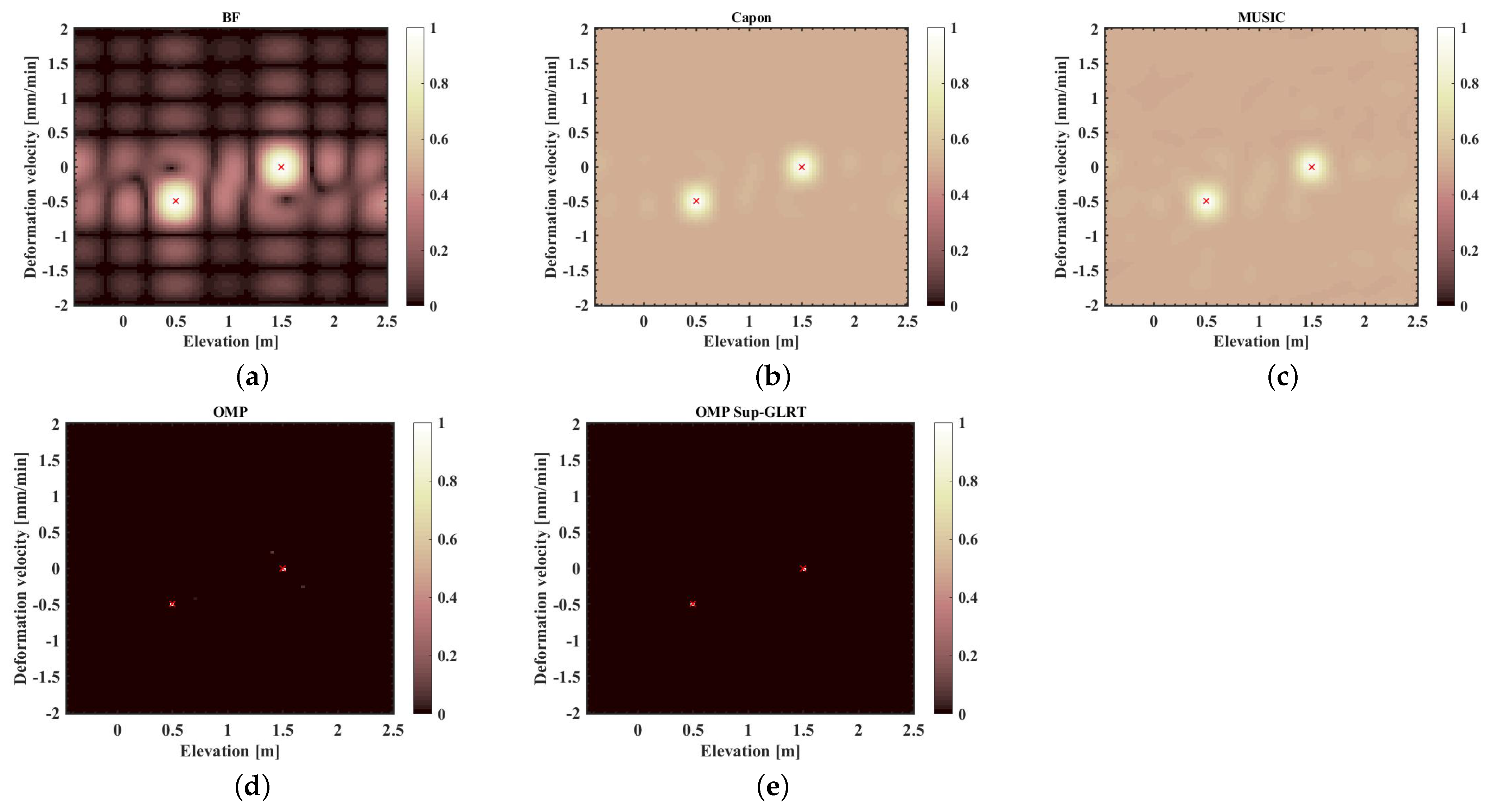
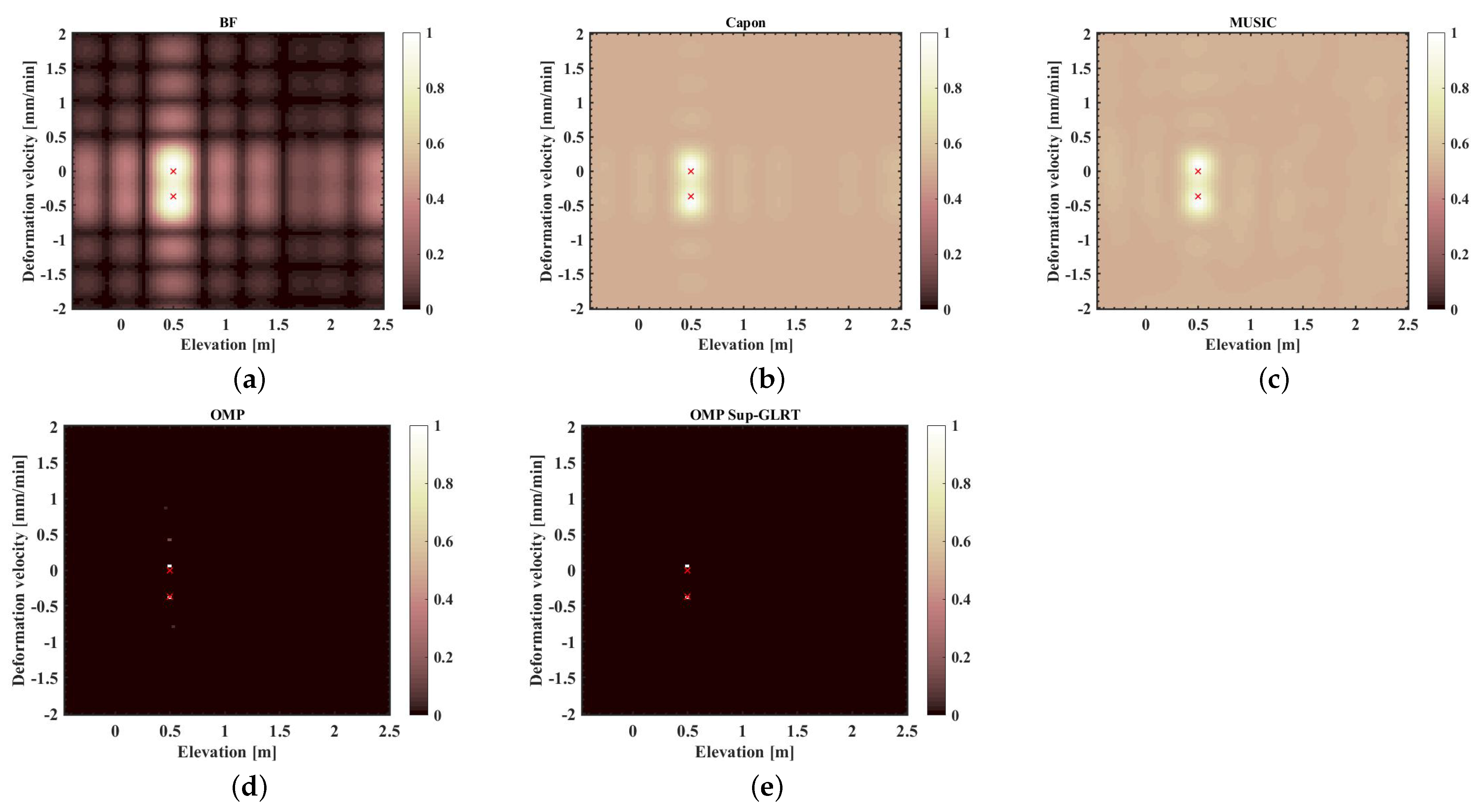
5.2.1. Simulation

In this section, several experiments based on the simulated data are used to validate the proposed method. The results of different kinds of imaging methods, such as BF, Capon, MUSIC, and OMP are used for comparison with the image recovered by the proposed method. The simulated parameters are identical to the ones of GOTCHA. A sub-aperture with a division was selected here, which has an azimuth angle of 6°. The average values of the slant range and incident angle were taken from this sub-aperture for conducting subsequent simulations. In the simulation, the No.8 SAR image is selected as the master one. The baseline distribution is shown in Table 4 and the mean elevation angle is 44.9013°. Assuming a pixel unit contains two scatterers with elevation positions s 1 = 0.5 m and s 2 = 1.5 m, the S N R = 15 dB, ρ s 0.5 m , ρ v 33.4 mm/h. Figure 7 shows the amplitude-normalized TomoSAR imaging results of BF, Capon, MUSIC, OMP, and OMP Sup-GLRT algorithms, respectively. It can be observed that the sidelobes of spectral estimation algorithms are serious. Although the OMP algorithm can effectively suppress these sidelobes, some error signals also appear. Meanwhile, the proposed OMP Sup-GLRT method can realize the screening of the OMP result, and remove the error signal according to a certain false alarm rate. When the distance between two scatterers is smaller than the elevation’s theoretical resolution ( s 1 = 0.5 m, s 2 = 0.75 m), as shown in Figure 8, it is observed that the proposed method can not only accurately identify the scatterers, but also has the super-resolving capability.
Setting the deformation velocity and elevation position of the two scatterers in a pixel unit as (0.5 m, −0.5 mm/min), (1.5 m, 0 mm/min), respectively (please observe the positions marked by the red asterisks in Figure 9). It is observed that all five methods can accurately identify the elevation position and deformation velocity of the scatterers. However, the recovered images of OMP and the proposed method have less sidelobes. Then, we set s 1 = (0.5 m, −3.7 mm/min), s 2 = (0.5 m, 0 mm/min) where the deformation velocity interval of scatterers is smaller than the theoretical resolution in Figure 10. It is found that the proposed method can still accurately identify the elevation position and deformation velocity of the scatterers, and achieve super-resolution imaging. This demonstrates that the proposed method has a better performance in sidelobe suppression and super-resolving imaging in D-TomoSAR.

5.2.2. Point Cloud Filtering

The point cloud statistical outlier removal (SOR) filtering method calculates the average distance from each point in the point cloud to the nearest m points, as well as the mean and variance of the average distance. The value of m is determined based on the number of points in the point cloud of the specific area that requires filtering in the experimental scene [42]. Based on the mean and variance of the calculated average distance, points with a distance greater than l ± k σ are identified as noise and are removed; where l represents the mean value and k is the noise denoising coefficient, generally the value is 1, 2, 3 and σ represents the variance.
Assuming q i ( x i , y i , z i ) is any point within the point cloud, where i = 1 , 2 , 3 , , n , and q i j ( x i j , y i j , z i j ) is any point in the neighborhood of point q i , where j = 1 , 2 , 3 , , m , then the average distance between point q i and other m neighbor points q i j can be written as
l i = 1 m j = 1 m ( x i x i j ) 2 + ( y i y i j ) 2 + ( z i z i j ) 2 .
The mean value of l i is
l i = 1 n i = 1 n l i
and the standard deviation of the average distance is
σ = 1 n i = 1 n l i l i 2
Assuming the average distance l i of point q i follows Gaussian distribution, i.e., l i N l i , σ 2 . Assuming d = l ± k σ is the average distance threshold, and k = 1 . The point whose average distance is less than or equal to d will be retained. Otherwise, it will be regarded as noise and removed.
The SAR image of the whole scene of GOTCHA dataset is shown in Figure 11. The selected area is indicated by the red rectangle, whose SAR and optical images are shown in Figure 12. Figure 13a depicts the 3-D point cloud of the selected area reconstructed by the proposed method without point cloud filtering. The red box highlights some outliers in the image. After performing filtering, as shown in Figure 13b, it can be observed that the new image eliminates the outliers present in Figure 13a, leading to a more standardized and accurate 3-D point cloud. This facilitates a more precise scatterer extraction for the subsequent 4-D inversion.

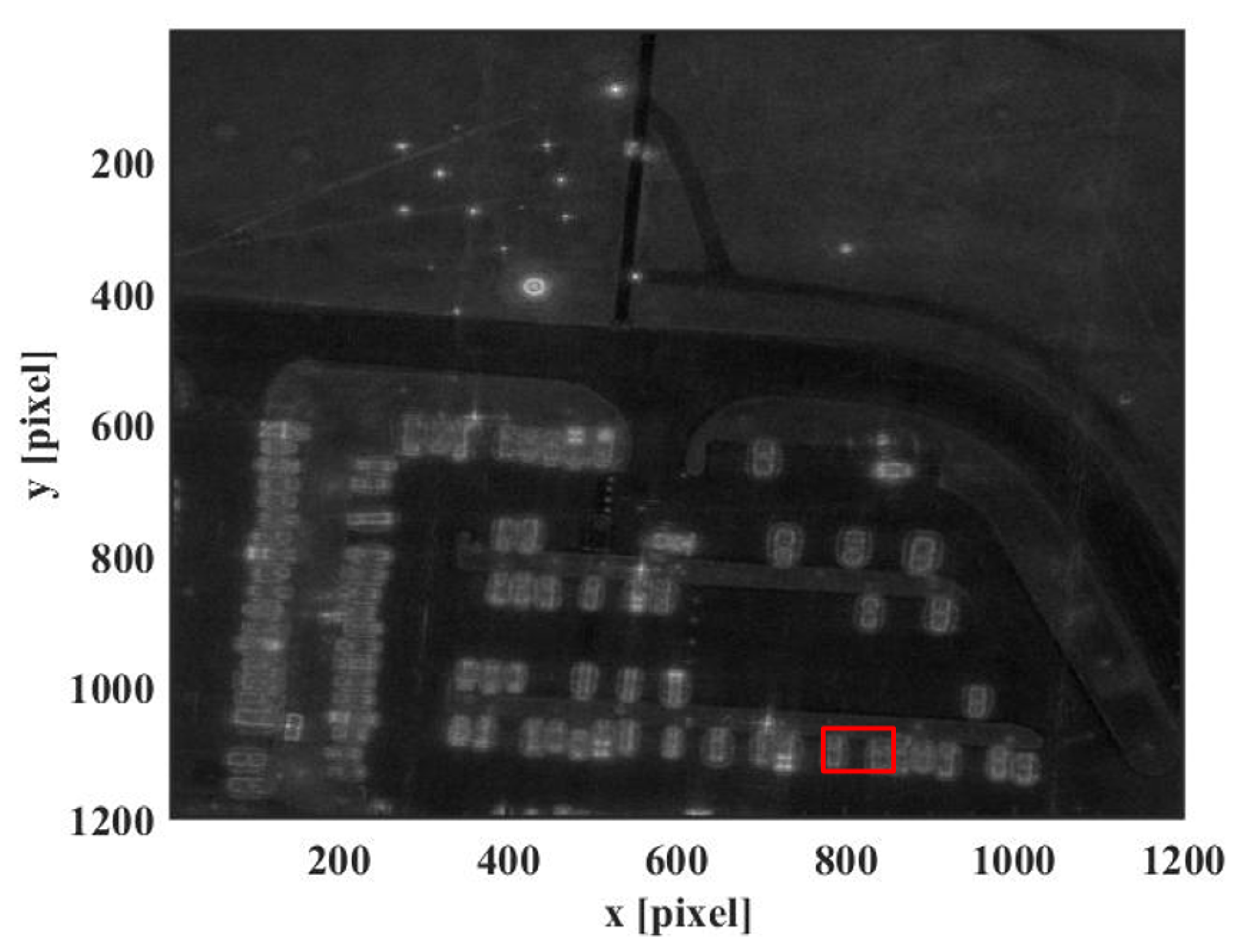
5.2.3. Real Data Experiment

The vehicle flow rate in the GOTCHA dataset can reach up to about 1.5 m every 4 min. However, the differential HoloSAR imaging is not suitable for detecting changes in this dataset due to system constraints and a short time baseline. Additionally, the short time duration reduces the significance of change detection in this dataset. Since the change of the vehicle can be clearly observed from eight SAR images, this paper reconstructs the changed scene in 3-D according to the change of the vehicle shown in the SAR image and then reconstructs the size of the deformation. The 3-D results of several methods in this paper are shown in Figure 14. We can observe that the images of spectral estimation methods have serious background artifacts due to the excessive sidelobes, and the OMP-based result has some outliers due to the inaccurate identification of scatterers. Meanwhile, the proposed OMP Sup-GLRT method can accurately identify the scatterers on the vehicle, effectively remove outliers, and reflect the real 3-D structure of the selected area.
Figure 15 shows eight SAR images of the selected area. It can be observed that there are two cars in scenes No.1 to No.4, but there are changes in scenes No.5 to No.8, leaving only a car. Figure 16 shows the 3-D point clouds recovered by the data of No.1 to No.8, No.1 to No.4, and No.5 to No.8, respectively. For the changed vehicle, the result of Figure 16a is worse than that of Figure 16b because the vehicle undergoes changes in scenes No.1 to No.8 while remaining unchanged in the first four scenes. Since the two cars are always present in scenes No.1 to No.4, Figure 16b can clearly show the 3-D result of the two cars. From Figure 16c, it can be observed that one car has left, indicating that there is only one car left in scenes No.5 to No.8, which is consistent with the actual situation. By using the subtraction method, the change of vehicles from No.1 to No.8 scenes in this area is more intuitively displayed, as shown in Figure 17. The color bar indicates the magnitude of the change, and a negative value indicates that the vehicle has left.
To further observe the vehicle variations throughout the whole scene, Figure 18 shows the 3-D reconstruction result of a large-scale scene by using the data of all eight scenes. Figure 19 shows the result by using only four scenes of data. It is evident that the reconstruction quality with four scenes is significantly inferior to that with eight scenes. The red boxes in the images indicate the vehicles that have undergone changes. These two vehicles are present in scenes No.1 to No.4 but have been left by scenes No.5 to No.8. In Figure 19, it can be observed that these two vehicles are no longer present. By employing different numbers of 2-D SAR images for scene reconstruction, we can not only obtain the 3-D elevation information of vehicles but also detect the changes in some vehicles. This provides a foundation for further extending the application of this method to a broader range of scenarios.

6. Discussion

Due to the short-time baselines of the dataset, the differential HoloSAR imaging technique was not used in actual experiments. Further follow-up research can focus on exploring the potential of differential HoloSAR technology and applying it to a suitable dataset to verify its effectiveness. Additionally, this imaging technique holds promise for future expansion in post-disaster reconstruction. For example, it can be applied to solve challenges such as the all azimuth angle deformation of buildings after earthquakes, thus providing valuable technical support for post-disaster reconstruction work.

7. Conclusions

HoloSAR is an attractive imaging mode that combines CSAR and TomoSAR imaging techniques to achieve all azimuth angle 3-D reconstruction of objects in the observed scene. Based on HoloSAR, this paper presents a differential HoloSAR imaging model and proposes a HoloSAR and differential HoloSAR imaging method based on OMP Sup-GLRT. The proposed method was applied to the GOTCHA dataset and achieved a high-precision 3-D reconstruction of parking lots. Compared with the classical spectral estimation algorithms, the proposed method can realize the super-resolution reconstruction of the elevation and deformation velocity, whose super resolutions are 2 times and 1.49 times, respectively. In addition, compared with the OMP algorithm, the proposed method can effectively filter out the incorrect scatterers with a constant false alarm rate, resulting in more accurate scattering information. Furthermore, the SOR filtering technology is employed for post-processing the point cloud, leading to the improved accuracy of the reconstructed 3-D result. The paper also utilizes the changed SAR image to derive the 3-D point cloud based on the vehicle flow in the SAR image. By performing subtraction, the change in vehicle size is determined across eight scenes. In future research, the differential HoloSAR imaging model can be directly employed for 4-D reconstruction on a suitable dataset, enabling the acquisition of high-precision 3-D and 4-D images.

Author Contributions

S.J., H.B. and J.Z. conceived the article. S.J., J.F. and W.X. processed the GOTCHA data and performed related experiments. S.J., H.B., J.F., W.X. and J.X. participated in the writing of this article. All authors have read and agreed to the published version of the manuscript.

Funding

This work was supported by the National Natural Science Foundation of China under Grant 62271248 and Guangdong Basic and Applied Basic Research Foundation under Grant 2020B1515120060.

Data Availability Statement

The GOTCHA dataset comes from the Civilian Parking Lot dataset released by the United States Air Force Research Laboratory.

Acknowledgments

The author would like to thank the United States Air Force Research Laboratory for providing the GOTCHA dataset.

Conflicts of Interest

The authors declare no conflict of interest.

Abbreviations

The following abbreviations are used in this manuscript:
SAR Synthetic Aperture Radar
CSAR Circular Synthetic Aperture Radar
MCSAR Multi-circular Synthetic Aperture Radar
2-D Two-dimensional
3-D Three-dimensional
4-D Four-dimensional
InSAR Interference SAR
TomoSAR SAR Tomography
D-TomoSAR Differential SAR Tomography
CS Compressive Sensing
HoloSAR Holographic SAR Tomography
BF Beamforming
Capon Adaptive Beamforming
MUSIC Multiple Signal Classification
OMP Orthogonal Matching Pursuit
RIP Restricted Isometric Property
GLRT Generalized Likelihood Ratio Test
Sup-GLRT Support Generalized Likelihood Ratio Test
CFAR Constant False Alarm Rate
SOR Statistical Outlier Removal
BIC Bayesian Information Criterion
SNR Signal-to-noise Ratio
BP Back-projection

References

  1. Soumekh, M. Reconnaissance with slant plane circular SAR imaging. IEEE Trans. Image Process. 1996, 5, 1252–1265. [Google Scholar] [CrossRef] [PubMed] [Green Version]
  2. Tsz-King, C.; Kuga, Y.; Ishimaru, A. Experimental studies on circular SAR imaging in clutter using angular correlation function technique. IEEE Trans. Geosci. Remote Sens. 1999, 37, 2192–2197. [Google Scholar] [CrossRef]
  3. Ponce, O.; Prats, P.; Scheiber, R.; Reigber, A.; Moreira, A. Multibaseline 3-D circular SAR imaging at L-band. In Proceedings of the 9th European Conference on Synthetic Aperture Radar, Nuremberg, Germany, 23–26 April 2012. [Google Scholar]
  4. Ponce, O.; Prats, P.; Scheiber, R.; Reigber, A.; Moreira, A. First demonstration of 3-D holographic tomography with fully polarimetric multi-circular SAR at L-band. In Proceedings of the IEEE International Geoscience and Remote Sensing Symposium, Melbourne, VIC, Australia, 21–26 July 2013. [Google Scholar]
  5. Ponce, O.; Prats-Iraola, P.; Pinheiro, M.; Rodriguez-Cassola, M.; Scheiber, R.; Reigber, A.; Moreira, A. Fully polarimetric high-resolution 3-D imaging with circular SAR at L-band. IEEE Trans. Geosci. Remote Sens. 2014, 52, 3074–3090. [Google Scholar] [CrossRef]
  6. Ponce, O.; Prats, P.; Scheiber, R.; Reigber, A.; Moreira, A. Study of the 3-D impulse response function of holographic SAR tomography with multi circular acquisitions. In Proceedings of the 10th European Conference on Synthetic Aperture Radar, Berlin, Germany, 3–5 June 2014. [Google Scholar]
  7. Bao, Q.; Lin, Y.; Hong, W.; Zhang, B. Multi-circular synthetic aperture radar imaging processing procedure based on compressive sensing. In Proceedings of the The 4th International Workshop on Compressed Sensing Theory and its Applications to Radar, Sonar and Remote Sensing, Aachen, Germany, 19–22 September 2016. [Google Scholar]
  8. Ponce, O.; Prats-Iraola, P.; Scheiber, R.; Reigber, A.; Moreira, A. First airborne demonstration of holographic SAR tomography with fully polarimetric multi circular acquisitions at L-band. IEEE Trans. Geosci. Remote Sens. 2016, 54, 6170–6196. [Google Scholar] [CrossRef]
  9. Budillon, A.; Schirinzi, G. GLRT based on support estimation for multiple scatterers detection in SAR tomography. IEEE J. Sel. Top. Appl. Earth Obs. Remote Sens. 2016, 9, 1086–1094. [Google Scholar] [CrossRef]
  10. Chen, L.; An, D.; Huang, X.; Zhou, Z. A 3D reconstruction strategy of vehicle outline based on single-pass single-polarization CSAR data. IEEE Trans. Image Process. 2017, 26, 5545–5554. [Google Scholar] [CrossRef] [PubMed]
  11. Bao, Q.; Lin, Y.; Hong, W.; Shen, W.; Zhao, Y.; Peng, X. Holographic SAR tomography image reconstruction by combination of adaptive imaging and sparse Bayesian inference. IEEE Geosci. Remote Sens. Lett. 2017, 14, 1248–1252. [Google Scholar] [CrossRef]
  12. Feng, D.; An, D.; Huang, X.; Li, Y. A phase calibration method based on phase gradient autofocus for airborne holographic SAR imaging. IEEE Geosci. Remote Sens. Lett. 2019, 16, 864–1868. [Google Scholar] [CrossRef]
  13. Feng, D.; An, D.; Chen, L.; Huang, X. Holographic SAR tomography 3-D reconstruction based on iterative adaptive approach and generalized likelihood ratio test. IEEE Trans. Geosci. Remote Sens. 2021, 59, 305–315. [Google Scholar] [CrossRef]
  14. Wang, M.; Wei, S.; Zhou, Z.; Shi, J.; Zhang, X.; Guo, Y. CTV-Net: Complex-valued TV-driven network with nested topology for 3-D SAR imaging. IEEE Trans. Neural Netw. Learn. Syst. 2022, 1–15. [Google Scholar] [CrossRef]
  15. Smith, J.W.; Torlak, M. Deep learning-based multiband signal fusion for 3-D SAR super-resolution. IEEE Trans. Aerosp. Electron. Syst. 2023, 1–17. [Google Scholar] [CrossRef]
  16. Reigber, A.; Moreira, A.; Papathanassiou, K.P. First demonstration of airborne SAR tomography using multibaseline L-band data. In Proceedings of the IEEE International Geoscience and Remote Sensing Symposium, Hamburg, Germany, 28 June–2 July 1999. [Google Scholar]
  17. Reigber, A.; Moreira, A. First demonstration of airborne SAR tomography using multi baseline L-band data. IEEE Trans. Geosci. Remote Sens. 2000, 38, 2142–2152. [Google Scholar] [CrossRef]
  18. Lombardini, F. Differential tomography: A new framework for SAR interferometry. IEEE Trans. Geosci. Remote Sens. 2005, 43, 37–44. [Google Scholar] [CrossRef]
  19. Fornaro, G.; Serafino, F.; Reale, D. 4-D SAR imaging: The case study of Rome. IEEE Geosci. Remote Sens. Lett. 2010, 7, 236–240. [Google Scholar] [CrossRef]
  20. Reale, D.; Fornaro, G.; Pauciullo, A. Extension of 4-D SAR imaging to the monitoring of thermally dilating scatterers. IEEE Trans. Geosci. Remote Sens. 2013, 51, 5296–5306. [Google Scholar] [CrossRef]
  21. Lombardini, F.; Viviani, F. New developments of 4-D+ differential SAR tomography to probe complex dynamic scenes. In Proceedings of the IEEE Geoscience and Remote Sensing Symposium, Quebec City, QC, Canada, 13–18 July 2014. [Google Scholar]
  22. Jo, M.-J.; Jung, H.-S.; Chae, S.-H. Advances in three-dimensional deformation mapping from satellite radar observations: Application to the 2003 bam earthquake. Geomat. Nat. Hazards Risk 2018, 9, 678–690. [Google Scholar] [CrossRef] [Green Version]
  23. Chai, H.; Lv, X.; Yao, J.; Xue, F. Off-grid differential tomographic SAR and its application to railway monitoring. IEEE J. Sel. Top. Appl. Earth Obs. Remote Sens. 2019, 12, 3999–4013. [Google Scholar] [CrossRef]
  24. Candès, E.J. Compressive sampling. Proc. Int. Congr. Math. 2006, 3, 1433–1452. [Google Scholar]
  25. Baraniuk, R.; Steeghs, P. Compressive radar imaging. In Proceedings of the IEEE Radar Conference, Waltham, MA, USA, 17–20 April 2007. [Google Scholar]
  26. Zhu, X.X.; Bamler, R. Super-resolution for 4-D SAR tomography via compressive sensing. In Proceedings of the 8th European Conference on Synthetic Aperture Radar, Aachen, Germany, 7–10 June 2010. [Google Scholar]
  27. Zhu, X.X.; Bamler, R. Superresolving SAR tomography for multidimensional imaging of urban areas: Compressive sensing-based TomoSAR inversion. IEEE Signal Process. Mag. 2014, 31, 51–58. [Google Scholar] [CrossRef]
  28. Wu, Y.Y.; Hong, W.; Zhang, B.C. Introduction to Sparse Microwave Imaging; Science Press: Beijing, China, 2018. [Google Scholar]
  29. Shi, Y.; Zhu, X.X.; Bamler, R. Nonlocal compressive sensing-based SAR tomography. IEEE Trans. Geosci. Remote Sens. 2019, 57, 3015–3024. [Google Scholar] [CrossRef] [Green Version]
  30. Chai, H.; Lv, X.; Xiao, P. Deformation monitoring using ground-based differential SAR tomography. IEEE Geosci. Remote Sens. Lett. 2020, 17, 993–997. [Google Scholar] [CrossRef]
  31. Lombardini, F.; Pardini, M. 3-D SAR tomography: The multibaseline sector interpolation approach. IEEE Geosci. Remote. Sens. Lett. 2008, 5, 630–634. [Google Scholar] [CrossRef]
  32. Zhu, X.X.; Bamler, R. Tomographic SAR inversion by L1-norm regularization—The compressive sensing approach. IEEE Trans. Geosci. Remote Sens. 2010, 48, 3839–3846. [Google Scholar] [CrossRef] [Green Version]
  33. Lin, Y.; Hong, W.; Tan, W.; Wang, Y.; Wu, Y. Interferometric circular SAR method for three-dimensional imaging. IEEE Geosci. Remote Sens. Lett. 2011, 8, 1026–1030. [Google Scholar] [CrossRef]
  34. Stoica, P.; Moses, R. Spectral Analysis of Signals; Pearson Prentice Hall: Upper Sadle River, NJ, USA, 2005. [Google Scholar]
  35. Capon, J. High-resolution frequency-wavenumber spectrum analysis. Proc. IEEE 1969, 57, 1408–1418. [Google Scholar] [CrossRef]
  36. Schmidt, R. Multiple emitter location and signal parameter estimation. IEEE Trans. Antennas Propag. 1979, 34, 276–280. [Google Scholar] [CrossRef] [Green Version]
  37. Stoica, P.; Arye, N. MUSIC, maximum likelihood, and Cramer-Rao bound. Acoust. Speech Signal Process. IEEE Trans. 1989, 37, 720–741. [Google Scholar] [CrossRef]
  38. Pati, Y.C.; Rezaiifar, R.; Krishnaprasad, P.S. Orthogonal matching pursuit: Recursive function approximation with applications to wavelet decomposition. In Proceedings of the 27th Asilomar Conference on Signals, Systems and Computers, Pacific Grove, CA, USA, 1–3 November 1993; pp. 40–44. [Google Scholar]
  39. Tropp, J.A.; Gilbert, A.C. Signal recovery from random measurements via orthogonal matching pursuit. IEEE Trans. Inf. Theory 2007, 53, 4655–4666. [Google Scholar] [CrossRef] [Green Version]
  40. Luo, H.; Li, Z.; Dong, Z.; Yu, A.; Zhang, Y.; Zhu, X. Super-resolved multiple scatterers detection in SAR tomography based on compressive sensing generalized likelihood ratio test (CS-GLRT). Remote Sens. 2019, 11, 1930. [Google Scholar] [CrossRef] [Green Version]
  41. Casteel, C.H., Jr.; Gorham, L.A.; Minardi, M.J.; Scarborough, S.M.; Naidu, K.D.; Majumder, U.K. A challenge problem for 2D/3D imaging of targets from a volumetric data set in an urban environment. SPIE 2007, 6568, 97–103. [Google Scholar]
  42. Guo, J.; Feng, W.; Hao, T.; Wang, P.; Xia, S.; Mao, H. Denoising of a multi-station point cloud and 3D modeling accuracy for substation equipment based on statistical outlier removal. In Proceedings of the 2020 IEEE 4th Conference on Energy Internet and Energy System Integration, Wuhan, China, 30 October–1 November 2020; pp. 2793–2797. [Google Scholar]
Figure 1. The imaging geometry of TomoSAR.
Remotesensing 15 03421 g001
Figure 2. The imaging principle of TomoSAR.
Remotesensing 15 03421 g002
Figure 3. The imaging geometry of D-TomoSAR.
Remotesensing 15 03421 g003
Figure 4. The imaging geometry of HoloSAR.
Remotesensing 15 03421 g004
Figure 5. Processing flow of the proposed method.
Remotesensing 15 03421 g005
Figure 6. Flow chart of the differential HoloSAR imaging.
Remotesensing 15 03421 g006
Figure 7. TomoSAR results based on simulated data by the different methods. (a) BF. (b) Capon. (c) MUSIC. (d) OMP. (e) The proposed OMP Sup-GLRT method. (Red asterisks indicate the set elevation positions of the scatterers; the blue line represents the simulated result).
Remotesensing 15 03421 g007
Figure 8. TomoSAR results based on simulated data by the different methods. (a) BF. (b) Capon. (c) MUSIC. (d) OMP. (e) The proposed OMP Sup-GLRT method. (The elevation interval of scatterers is smaller than the theoretical resolution).
Remotesensing 15 03421 g008
Figure 9. D-TomoSAR results based on simulated data by the different methods. (a) BF. (b) Capon. (c) MUSIC. (d) OMP. (e) The proposed OMP Sup-GLRT method.
Remotesensing 15 03421 g009
Figure 10. D-TomoSAR results based on simulated data by the different methods. (a) BF. (b) Capon. (c) MUSIC. (d) OMP. (e) The proposed OMP Sup-GLRT method. (The deformation velocity interval of scatterers is smaller than the theoretical resolution).
Remotesensing 15 03421 g010
Figure 11. SAR image of the whole scene.
Remotesensing 15 03421 g011
Figure 12. Selected area in Figure 11. (a) SAR image. (b) Optical image.
Remotesensing 15 03421 g012
Figure 13. Reconstructed 3-D point clouds of the selected area by the proposed method. (a) Before point cloud filtering. (b) After point cloud filtering.
Remotesensing 15 03421 g013
Figure 14. Reconstructed 3-D point clouds of the selected area by the different methods. (a) BF. (b) Capon. (c) MUSIC. (d) OMP. (e) The proposed OMP Sup-GLRT method.
Remotesensing 15 03421 g014
Figure 15. Eight SAR images of the selected area. (a) No.1. (b) No.2. (c) No.3. (d) No.4. (e) No.5. (f) No.6. (g) No.7. (h) No.8 (Master).
Remotesensing 15 03421 g015
Figure 16. Reconstructed 3-D point clouds of the selected area by the proposed method from different datasets. (a) The dataset consists of No.1 to No.8 2-D SAR images. (b) The dataset consists of No.1 to No.4 2-D SAR images. (c) The dataset consists of No.5 to No.8 2-D SAR images.
Remotesensing 15 03421 g016
Figure 17. Reconstructed 4-D image of the selected area by the proposed method. (a) Side view 45° result. (b) Side view result.
Remotesensing 15 03421 g017
Figure 18. Reconstructed point cloud of the large-scale scene by the proposed method from the dataset consists of all 8 SAR images.
Remotesensing 15 03421 g018
Figure 19. Reconstructed point cloud of the large-scale scene by the proposed method from the dataset consists of No.5 to No.8 SAR images.
Remotesensing 15 03421 g019
Table 1. Flow chart of the OMP-based TomoSAR imaging.
OMP Algorithm
  • Input the observation matrix Φ , the measurement vector g and the number of iterations K.
  • At the first iteration, set γ ^ = 0 and supp X 0 = .
  • After k iterations, set W k = Φ H g Φ · γ ^ k and find the position of the element with the
    largest modulus value of W k .
  • Update supp X k + 1 = supp X k arg min i W i k and
    γ ^ k + 1 = Φ supp X k + 1 H Φ supp X k + 1 1 Φ supp X k + 1 H g , where k = 1 , , K .
  • Output γ ^ k + 1 .
Table 2. Flow chart of the model selection.
Model Selection-Sup-GLRT Algorithm
  • Input the elevation distribution result γ ^ obtained by OMP algorithm and the measurement
    vector g .
  • Calculate Λ k and T k in (19).
  • Compare the sizes of Λ k and T k . If Λ k is greater than T k and k = k + 1 , continue cycling until
    k = K output and P k = K ; If Λ k is less than T k , output P k 1 .
Table 3. System parameters of the GOTCHA dataset.
WavelengthAverage Slant RangeAverage View AngleNumber of Data
0.0313 m10,168.2 m44.3°8
Table 4. Baseline distribution of eight SAR images.
SAR Image IDNo.1No.2No.3No.4No.5No.6No.7No.8 (Master)
Temporal baseline−28 min−24 min−20 min−16 min−12 min−8 min−4 min0 min
Elevation angle45.7485°45.5939°45.3287°−45.0614°44.7775°44.4165°44.2241°44.0594°
Disclaimer/Publisher’s Note: The statements, opinions and data contained in all publications are solely those of the individual author(s) and contributor(s) and not of MDPI and/or the editor(s). MDPI and/or the editor(s) disclaim responsibility for any injury to people or property resulting from any ideas, methods, instructions or products referred to in the content.

