Article

Comparison of Three Active Microwave Models of Forest Growing Stock Volume Based on the Idea of the Water Cloud Model

1
College of Geoscience and Surveying Engineering, China University of Mining and Technology-Beijing, Beijing 100083, China
2
Ningxia Data and Application Center of High Resolution Earth Observation System, Ningxia Institute of Remote Sensing Survey, Yinchuan 750021, China
3
Satellite Application Center for Ecology and Environment, Ministry of Ecology and Environment, Beijing 100094, China
*
Author to whom correspondence should be addressed.
Remote Sens. 2023, 15(11), 2848; https://doi.org/10.3390/rs15112848
Submission received: 14 March 2023 / Revised: 22 May 2023 / Accepted: 25 May 2023 / Published: 30 May 2023
(This article belongs to the Special Issue Remote Sensing for Soil Moisture and Vegetation Parameters Retrieval)

Abstract

:
Forest growing stock volume (GSV) is an essential aspect of ecological carbon stock monitoring. The successive launches of spaceborne microwave satellites have provided a broader way to use microwave remote sensing to monitor forest accumulation. Currently, the inversion parameterization models of active microwave remote sensing stock volume mainly include the interferometric water cloud (IWCM), BIOMASAR, and Siberia. Among them, the IWCM introduces backscattering and coherence, the BIOMASAR model only introduces backscattering, and the Siberia model only introduces coherence. Although these three models combine the backscatter coefficient and coherence of SAR to estimate volume accumulation, the performance of the models has not been evaluated at the same time in the same area. Therefore, this article starts from the perspective of the three combinations of coherence and backscattering, relies on three models that do not require measured data, and evaluates the accuracy of the models’ overall inversion of GSV. In addition, we combine precipitation meteorological information, vegetation types, and seasonal variation to separately explore model performance. The comparison results show that the IWCM model is relatively stable in the process of stock volume inversion and is more sensitive to the vegetation types of coniferous and deciduous forests. The influence of seasons and precipitation on the model is weak, and the accuracy of the multi-time-series model is slightly improved. The Siberia model has a good storage volume inversion effect in this study area, but the multiple time series did not improve the model accuracy. The BIOMASAR model is simple, and its performance was slightly inferior in this study area. Precipitation can negatively affect BIOMASAR. The model results for multiple time series outperform those for single time. In summary, the stability of IWCM is more suitable for research with unknown information. The BIOMASAR model is simple, does not require coherence calculations, and is ideal for the estimation of large-scale national or world-level storage distributions. The Siberian model performs better in small regions and smaller spatiotemporal baselines.

1. Introduction

Ecological issues are currently being investigated by almost all countries around the world [1,2,3]. Among these ecological issues, forests are an important research target because they play a vital role in regulating the ecological climate and are the primary means of carbon uptake [4,5,6]. The forest growing stock volume (GSV) is a critical parameter of a forest and is generally related to the forest economy and sustainable development [6,7]. The forest GSV refers to the total volume of standing trees in the forest per unit area, and the unit is usually cubic meters per hectare (m3/ha). Usually, GSV is measured in the field by manually collecting the breast diameter and tree height of the trees in a sample plot and then calculating an allometric equation or checking a height–breast diameter–volume table to estimate the GSV [8]. The manual field measurement method is time-consuming and labor-intensive, with long renewal cycles and limited working areas making it challenging to widely use.
With the continuous development of remote sensing science and technology, more and more works have estimated the GSV [9]. Currently, the GSV estimation methods in remote sensing mainly include passive optical remote sensing, active optical remote sensing, and active microwave remote sensing [10,11,12,13]. The passive optical remote sensing method is mainly based on combining spectral information with the measured data to carry out modeling regression to obtain the GSV [11,14,15]. However, passive optical remote sensing technology cannot obtain data all day in all weather, visible light cannot pass through clouds and fog, and is easily affected by weather. Consequently, the direct sensitivity of the visible-light band to GSV is low, and high accuracy cannot be achieved. Active optical remote sensing mainly uses LiDAR for GSV estimation. LiDAR is mainly used to extract the vertical forest structure, distribution density, and other information through the point cloud and is combined with a digital elevation model (DEM) to obtain the GSV of a sample through multiple linear regression or machine learning [10,16,17,18,19]. Due to the effects of weather and the expensive data acquisition over a large area, LiDAR technology is also limited in application. In contrast, active microwave remote sensing can penetrate clouds and fog and acquire data in all weather, and microwaves are directly sensitive to GSV or biomass [20]. Moreover, it is becoming increasingly convenient to obtain microwave data as global microwave remote sensing satellites have been launched one after another in recent decades. The National Aeronautics and Space Administration (NASA) provides free passive microwave data from satellites such as SMAP and AMSR. The launch of the Sentinel-1 satellite has also provided new opportunities for active microwave remote sensing [21].
With the improvement in computing power, machine learning and deep learning algorithms are gradually being enriched, and these methods have been gradually introduced into the calculation of remote sensing parameters [22,23,24]. Currently, the commonly used methods for the inversion of forest GSV via active microwave remote sensing can be roughly divided into two categories: nonparametric and parametric models [25]. The nonparametric models introduce various field and microwave data parameters into the model and continuously train and correct the model to obtain the accumulation result [26,27,28,29,30]. Such models can often be highly accurate by combining a large amount of measured data with machine learning algorithms. To date, most studies have combined C- or L-band synthetic aperture radar (SAR) data with nonparametric machine learning algorithms to calculate GSV or biomass, mainly including random forest (RF) [26,27], support vector regression (SVR) [28], artificial neural network (ANN) [31], deep neural network (DNN) [27], and bagging stochastic gradient boosting (BagSGB) [32]. These methods are flexible and highly precise but produce poor interpretation and are prone to overfitting. The locally trained nonparametric models are challenging to directly use in other research areas, and these models rely on measured data. A parametric model refers to a model equation established by analyzing the relationship between microwave and ground objects. Although the usually established parametric model equations are relatively simple, the model can be improved and optimized by reasonably changing the parameters of the equations [33,34,35]. For instance, the water cloud model is one of the classical parametric models used for forest GSV inversion. This model describes the backscattering mechanism of SAR, revealing the scattering process of active microwaves to a certain extent. This model also describes the total amount of backscattering as a two-part contribution of bare soil and forest, which is weighted by forest transmittance to obtain the forest volume [36]. The water-cloud model has been applied to forest stock volumes in Sweden, Finland, and other places. The use of long-term time series and multi-time-series intensity data can produce better estimation results. For example, the BIOMASAR method combines the intensity information of multiple time series with the vegetation coverage to estimate the GSV without relying on the measured information [37,38]. A global GSV dataset in 2010 was produced by the BIOMASAR estimation model combined with the multi-time-series Envisat ASAR backscatter data, which has been of great help to studies without in situ measurements [9]. The water-cloud model was first proposed to calculate the vegetation canopy’s water content and soil moisture [39]. Based on this model, the coherence of SAR is introduced, the coherence of microwave is weighted by backscattering, and the forest volume is estimated from the perspective of the forest structure. A representative of this method is the interferometric water-cloud model (IWCM) [13,40,41]. The IWCM has achieved good results in estimating the GSV from C-band active microwave data and can be used for large-scale forest stock mapping [42]. Through the allometric growth equation, the interferometric water-cloud model has also been applied to the inversion of forest biomass. In combination with the relationship between tree height and forest volume, this model can also be used for tree height estimation, although the acquisition of SAR data is not limited. Strong wind can affect the shape of forest trees, which then affects the coherence of two SAR images. Precipitation affects the backscattering intensity information, so a model combined with multi-time-series data often produces better results [21,34,43]. In Siberia’s large-scale forest volume mapping, the IWCM was simplified, and a simple index model based on forest coherence was obtained, called the Siberia model [13,42,44,45]. The Siberia model, in combination with the estimation results of ERS-1/2 data, was proven reasonable [42], but there is no relevant research on multi-time-series data.
The above models are based on different combinations of radar backscatter coefficients and radar coherence coefficients. However, very few studies have evaluated the existing methods from the perspectives of only using backscatter, combining backscatter and coherence, and only using coherence. Because of this deficiency, it is still unclear how suitable models can be selected to estimate GSV with active microwave remote sensing. Consequently, this study focused on comparing the typical models of estimating the GSV from the above three perspectives. Specifically, the BIOMASAR model is a representative of using only backscatter, the IWCM model is a representative of using coherence and backscatter, and the Siberia model is a representative of using only coherence; the three models do not need to use measured data in the process of calculating the GSV. This study contributes not only to better understanding the advantages, disadvantages, and applicability of existing methods in estimating the GSV with microwave remote sensing but also to finding directions for further improvement.

2. Materials and Methods
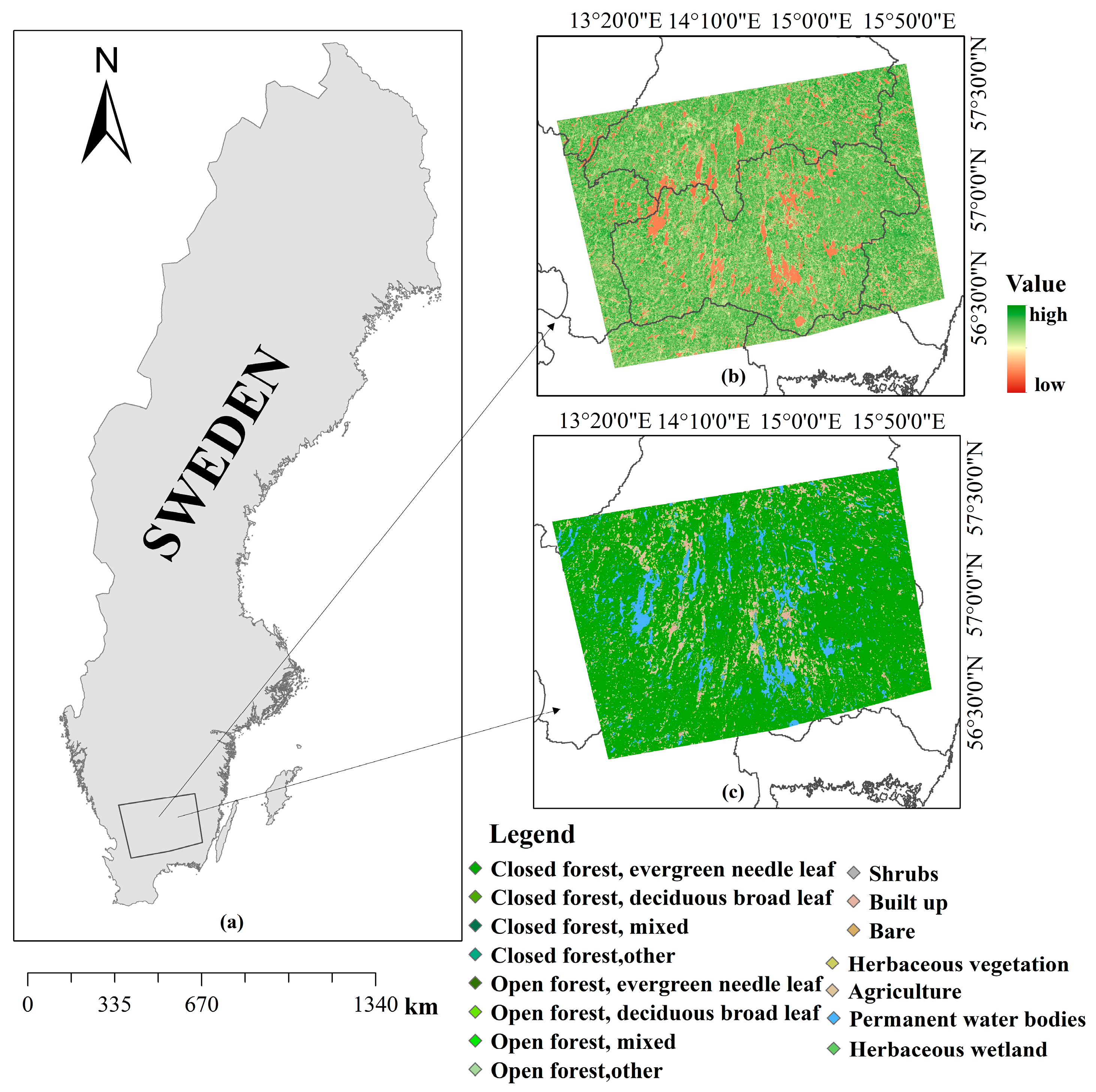
2.1. Study Area

In the past century, the total number of forests in Sweden has doubled, and the state of the ecological environment has also tended to improve. This is closely related to the acquisition of Sweden’s open natural resource survey data. Scholars and citizens can understand the local ecological conditions through public information. Therefore, this study comprehensively considered the data factors. Most of Kronoberg and some areas of surrounding cities were selected as the research area. The research area is shown in Figure 1.

2.2. Data

To better explore the performance of the model, we used C-band Sentinel-1 data as the main data; the Sentinel-2, DEM, and land cover data as auxiliary data; and the meteorological data and national forest inventory (NFI) ground point data as the data for evaluating the results.

2.2.1. Ground Point Data

This experiment did not depend on measured data in the processes of model establishment and estimation. Instead, measured data were only used in the processes of model evaluation and comparison. The data used in this experiment were a subset of the 2016 National Forest Inventory (NFI) sample plot data in Sweden. Each point in the sample plot data represents the forest situation of a circular plot with a radius of 7 m centered on this point. The dataset includes forest volume and records multiple attributes such as tree height, number of tree species, dry wood, and wet weight. We chose the southern part of Sweden, where the sampling points are densely distributed. In this research area, the central ecological communities are temperate broad-leaved forests and mixed forests, and forest species are relatively rich.

2.2.2. Sentinel Data

Sentinel data are the most widely used data in current research. The Sentinel-1 satellite was launched in 2014, and the strip scan mode includes stripmap (SM), interferometric wide swath (IW), extra-wide swath (EW), and wave (WV) modes. Among them, the WV scanning mode can only obtain single-polarization HH or VV model data, and other models can obtain single-polarization and dual-polarization data. A whole year of data were available for the study area in 2016. Therefore, to explore the impact of changes in the coherence and backscattering caused by changes in time and seasons on the estimation of the annual forest stock volume, we used the Sentinel_1A single-look complex (SLC) data from the IW scanning mode and VV polarization mode in 2016. There were 2 pieces of data per month, and the time baseline was 12 days. With a restricted baseline of 12 days, 18 pairs of coherence maps and 24 intensity maps of backscatter information were obtained.
The Sentinel-2 satellite was launched in 2015. The satellite is equipped with a multispectral imager, which can obtain 13 spectral bands, and the resolution of each band is different. Sentinel-2 multispectral data can be used to observe natural disasters such as volcanic eruptions, floods, and landslides. We used the SNAP and Sen2Cor (https://step.esa.int/main/, accessed on 1 March 2022) plugins provided by the ESA to perform radiometric calibration and atmospheric correction on the Sentinel-2L1C data and convert them into Sentinel-2L2A data for the calculation of vegetation coverage metadata. The obtained vegetation coverage was used to mask the parameters of the GSV inversion model.

2.2.3. Digital Elevation Model (DEM)

We used the 90 m resolution SRTM digital elevation model public data (https://www.earthdata.nasa.gov/sensors/srtm, accessed on 1 March 2022), which cover 80% of the world’s surface area. On the Swedish site, the data only cover the southern part of Sweden, which is one of the reasons why this research area was selected.

2.2.4. Land Cover Data

To minimize the influence of other land cover types on the result, we referred to the Copernicus Global Land Service: Land Cover 100 m: collection 3: epoch 2016: Globe (https://lcviewer.vito.be/2016, accessed on 1 March 2022) [46]. This dataset contains land surface classification data from 2015 to 2019. The research area data are shown in Figure 1c. The land surface can be divided into 23 categories, and the resolution is 100 m. The land cover data were used to mask the backscatter and coherence data in the experiment, and we only counted the part where the coverage type was forest.

2.2.5. Meteorological Data

The meteorological data were obtained from the official website of the National Center for Environmental Information, and the daily meteorological data in 2016 were obtained from the global surface summary of day data at (https://www.ncei.noaa.gov/maps/daily/, accessed on 1 May 2022). The data were obtained through 4 data collections per day, including multiple attributes such as daily average temperature, maximum and low temperature, precipitation, and dew point temperature. The global surface summary of the daily data is a comprehensive surface dataset that records the daily weather in detail. In this experiment, data extraction was performed according to the time and location of the SAR data.

2.3. Methods

The basic model in this study was the water-cloud model (WCM), which has been successfully applied in the inversion process of soil moisture, forest stock volume, and biomass [47]. The class water-cloud model used for forest parameter inversion is a simple backscattering parameter model, and the basic formula is as follows:
B f o r = B g r T t h r + B v e g ( 1 T t h r )
where B f o r is the total backscattering coefficient (dB); parameters B g r and B v e g represent the contribution of bare soil and vegetation to the backscattering (dB), respectively; and T t h r is the transmittance of microwaves through the forest.
T t h r = 1 f ( 1 T t r e e )
T t r e e = e α h
Here, f is the area filling factor; α is the attenuation factor of the forest, which represents the two-way attenuation per meter (dB/m); and T t r e e represents the two-way transmission rate of the forest. After verification [40,48], the transmission rate of the forest T t h r can be expressed as
T t h r = e β V o l
where V o l represents the forest stock volume (m3/ha), and β is the empirical coefficient (dimensionless). Then, we have
e β V o l = 1 f ( 1 e α h )
f = 1 e β V o l 1 e α h
We assume that the two-way transmittance of the forest is negligible [40]:
T t h r = e β V o l 1 f
The basis for this assumption is that the two-way attenuation of the forest in the C band a few meters before the canopy height of the forest is negligible [43]; then, the expression of the water-cloud model for forest stock volume inversion is
B f o r = B g r e β V o l + B v e g ( 1 e β V o l )

2.3.1. Interferometric Water-Cloud Model (IWCM)

The interferometric water-cloud model (IWCM) is mainly used for the inversion of forest stock volume and biomass. Its basic idea is similar to that of the water-cloud model. The coherence is divided into two parts that are contributed by vegetation and ground, separately, which are weighted by their respective backscattering. The vegetation contribution also considers the influence of the structure on volume decorrelation [25].
C f o r = C g r B g r B f o r T t h r + C v e g B v e g B f o r ( 1 T t h r ) C v o l
C v o l = α ( α j ω ) ( e j ω h e α h ) ( 1 e α h )
Here, C f o r is the total coherence, C g r is the time-dependent coherence of the ground, C v e g is the time-dependent coherence of trees, and the coherence is weighted by the backscattering, volume decorrelation, and geometric effects that the model considers. The first half of Equation (9) is the ground coherence contribution, and the second half represents the vegetation contribution, where ω is the geometric coefficient of the SAR image pair.
ω = 4 π B λ R sin θ
Here, B represents the normal component of the baseline, λ is wavelength, R is the slant range, and θ is the local incidence angle.

2.3.2. Siberia Model

The Siberia model has been validated in Siberia. Based on the IWCM, the model assumes that the spatial baseline is zero, and the backscattering intensity of each part is equal without considering the geometric effect of the interference and the decorrelation effect of the volume. The following simplified model was obtained [42,49]:
C f o r = C 0 e V ν V o l + C ( 1 e V ν V o l )
where exp ( V ν V o l ) is the exponential change relationship between the stock volume and coherence, V ν is the rate of coherence decrease with the increase in forest stock volume, C 0 is the coherence when the forest stock volume is zero, and C is the situation when the forest is extremely dense and saturated.

2.3.3. BIOMASAR Model

The basis of the BIOMASAR model is Equation (1). Considering that the model parameters of forest accumulation on a single date are easily affected by meteorological factors, the uncertainty of a single result is offset through the cumulative average of multi-time-series data [37].
V i = 1 β ln B v e g i B f o r i B v e g i B g r i
Here, i is the serial number of a certain time image in the time series; V i is the single-date accumulation result corresponding to the time; B f o r i corresponds to the total backscatter coefficient; and B v e g i and B g r i are the corresponding backscatter contributions of the vegetation and the ground, respectively. Parameter β is the empirical coefficient. The weighted average of the backscattering coefficients on the single-date stock volume can be used to obtain the final forest stock volume [20,25].
V M T = i = 1 N B i B max V i i = 1 N B i B max
Here, V M T is the multi-time-series GSV estimation result, B i = ( B v e g i B g r i ) i ; and B max is the maximum value of B i .

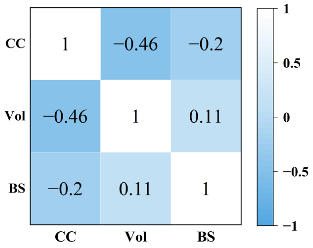
2.4. Parameter Determination

Figure 2 demonstrates the general experimental procedure used in this study. The known parameters in the three models were the total backscatter and coherence. Parameters B g r and C g r were determined using the vegetation coverage (VCF) data as a mask, and the VCF was calculated from Sentinel-2L2A data using SNAP software from European Space Agency (ESA). The threshold was set according to the distribution of the VCF, and the pixels were marked as “ground” and “dense vegetation” according to the threshold. Using a sliding window, the mean value of the pixels marked as “ground” in the window was considered to be the ground contribution of the central pixel, and the mean value of the pixels marked as “dense vegetation” was the contribution of dense vegetation [37,38]. Due to the different regional data sources and methods for calculating the VCF, the threshold of the VCF was slightly adjusted according to the actual situation, but the processes were the same. Parameters B v e g and C v e g were determined by selecting B V C F and C V C F in the dense vegetation area, respectively, through training in a similar way to B g r and C g r , respectively. B V C F and C V C F were introduced as parameters into the WCM and the IWCM formulas, and the values of B v e g and C v e g were calculated. For the calculation method, we referred to [42,50,51]. The geometric parameters of SAR in the model were extracted during the interference; the β empirical parameter refers to the existing research on BIOMASAR and IWCM, which reported a value of 0.006 ha/m3 [37]. Parameter V ν is the decreasing value of coherence with the growth in forest stock volume, and the value in this study was 0.015 according to the references. Parameter α is the attenuation factor of the forest, and its value is 2 dB/m according to [50,51].

2.5. Evaluation Method

The basic aim of this experimental model comparison was to perform baseline estimation, interference, filtering, and geocoding on the Sentinel-1 SLC data to obtain the coherence and backscatter. Geocoded backscatter and coherence information were fed into the model to obtain estimates of the forest stock for single image pairs. The weighted average was then used to obtain the inversion results of multi-time-series forest stock volume. In this experiment, the mean absolute error (MAE), root mean square error (RMSE), and relative root mean square error (RRMSE) were used to evaluate the accuracy of the results. The parameter V ¯ t r u e represents the mean of the true value, m is the total number of verification points, and V o l represents the model valuation. The smaller the evaluation value, the better the performance of the model.
M A E = 1 m l = 1 m V o l V t r u e
R M S E = 1 m l = 1 m V o l V t r u e 2
R R M S E = 1 m l = 1 m V o l V t r u e 2 V ¯ t r u e
The evaluation of the model was carried out from three aspects. The first one was the evaluation of the overall accuracy and efficiency. The quantitative indicators of model accuracy for a single time serious and multiple time series were calculated, as well as the correlation between the results and the measured values. Then, the performance of the model at multiple time series and a single time was evaluated, and the model with the best overall performance was selected. Second, the model performance was evaluated under different vegetation cover types and combined with the NFI tree type attribute and GSV data. Because each NFI point represents the vegetation within the radius, the vegetation types that accounted for greater than 50 percent within the range were considered to be tree types at this point. The evaluation factors were separately calculated for the classified results to obtain the model performance under different vegetation types. Third, the evaluation factors were combined with weather information. The weather station data and model results on the same date were extracted. Then, different weather conditions were distinguished to calculate the evaluation value, and the model performance under different weather conditions was analyzed.

3. Results

Figure 3 shows the result map of the GSV obtained after remote sensing data preprocessing and model inversion. The classification style of the result was consistent with that of [42,51]. All three models carried out the inversion of the forest stock volume. Among them, Figure 3a is the 2010 global forest stock volume dataset (https://globbiomass.org/products/global-mapping/, accessed on 1 May 2022) [9]; Figure 3b is the multi-time-series result of IWCM; Figure 3c is the multi-time-series result of the Siberia model; and Figure 3d is the BIMOASAR estimation result. It can be seen from the figure that the BIOMASAR model underestimated the GSV around water bodies. The Siberia result in Figure 3c and the IWCM model result in Figure 3d are more similar to the distribution of the dataset in 2010. In order to more comprehensively compare and evaluate the model results, the result evaluation was divided into three aspects from the whole to refinement.

3.1. Result Accuracy Evaluation

The precision quantification factors were extracted from the period-by-period data of the three models. The forest stock volume was considered to be stable without human intervention in a year, so the measured value in 2016 was taken as the real value in a year. Each model to be evaluated had 18 single-date results, 1 multi-time series result, and 159 points. First, the correlation analysis was performed and statistics were calculated between the estimated value and the actual measured value of a single period of this research site. Figure 4 is a heat map of the correlation distribution, where he lighter the color, the higher the correlation. From Figure 4, it can be concluded that the overall correlation of the inversion results of the IWCM model in this study area was slightly higher than that of the other two models.
For the three models, we calculated the MAE, RMSE, and RRMSE point by point by date, as shown in Figure 5. From the perspective of the RMSE and RRMSE, the Siberia model performed better, but there were outliers in the model.
The correlation between multiple time series and the measured GSV data from the NFI were calculated. Figure 6 represents the 2010 dataset. It can be seen that the correlation between the IWCM and GSV data from the NFI was higher than that of the other two models, and the correlation of BIOMASAR was lower than that of the other results. The lower accuracy of BIOMASAR is directly due to the model using existing data parameters. As mentioned in [33,34], the parameters can be directly used.
The multi-time-series results synthesized by weighting and superimposing the single-date results of the model are shown in Table 1. The average absolute error, root mean square error, and relative root mean square error of the IWCM model were better, followed by those of BIOMASAR and Siberia.

3.2. The Effect of Precipitation

To explore the factors that affect the models’ estimation results, we introduced the weather station data at the time of data acquisition. Meteorological records were collected corresponding to the time of the experimental SAR data. A total of 18 days, of which 5 days had precipitation, were evaluated. In this experiment, a precision evaluation of the precipitation date and nonprecipitation date results of the three models was carried out. As shown in Figure 7, from the statistical graphs of the three precision evaluation factors, we can see that the GSV estimated by the Siberia model and IWCM was relatively stable and hardly affected by precipitation. Precipitation increased the error in the BIOMASAR results, indicating that the model was more sensitive to precipitation, and different precipitation conditions had a certain impact on the model results.

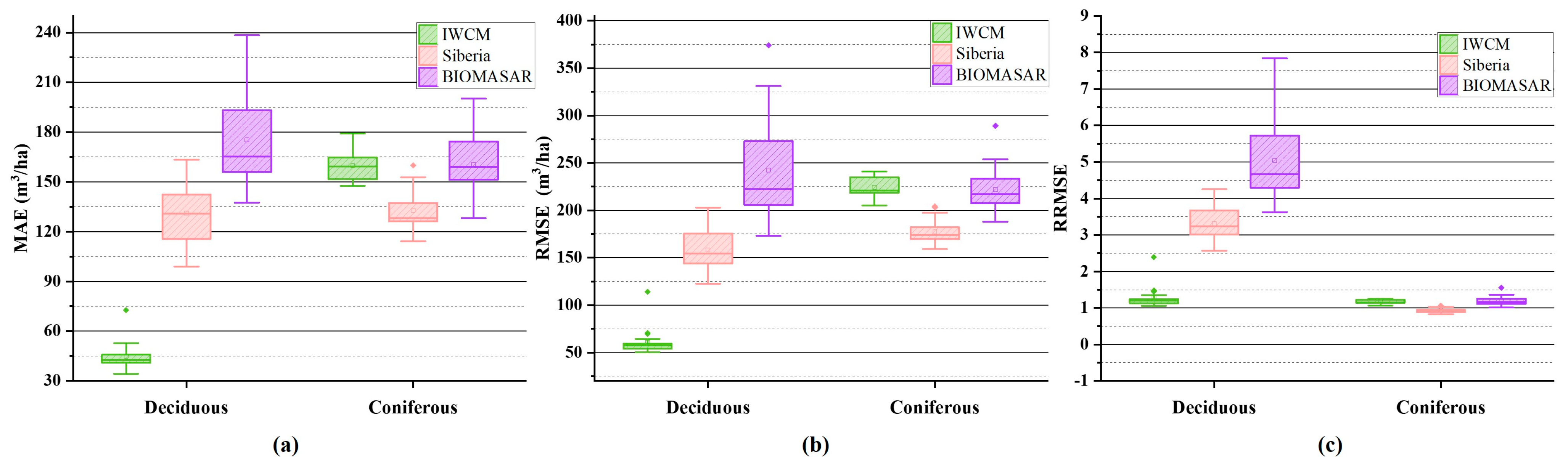
3.3. The Effect of Vegetation Type

From the measurement data, the volume points used for precision evaluation were artificially divided into coniferous and deciduous forests. The points of the forest resource survey data represent regional results, and each point represents a forest region with an area of about 154 square meters. Therefore, the tree species that contained more than 50% of the tree species were artificially defined as this point as the tree species represented by bits. According to manual statistics, among the 158 measured points, 111 measured points were coniferous forests, and the rest were deciduous forests. The point values of the estimation results were extracted for the stock volumes of the two types of tree species, and the separate accuracy evaluation factors were calculated. The final result is shown in Figure 8. It can be seen that the IWCM model was more sensitive to the type of tree species, and the model’s performance for coniferous forest was better than that for deciduous forest.

3.4. The Effect of Season

The 18-period data were divided according to the seasons in the Swedish regions by month. As the research area is located in southern Sweden, the division of months into the four seasons was roughly as follows: spring, March–May, containing four data; summer, June–August, containing five data; autumn, September–November, containing five data; winter, December–February, containing four data. Although the extraction time was 18 periods in total, the 159 points from each period of data were involved in the point accuracy evaluation. It can be seen from Figure 9 that the errors of the BIOMASAR model in the spring and winter were relatively high. This was because there were rainfall dates in the statistical results in these two seasons, so the model results considerably fluctuated. The error distribution of the Siberia model in each season was relatively low, but the model’s performance had certain fluctuations with the change of seasons. The IWCM model was less sensitive to the seasons, and the fluctuation was the least affected by the seasons.

4. Discussion

In this experiment, we used three existing models for comparison. Although the three models have been proven to successfully calculate the GSV, they have not been compared at the same time and in the same study area. In the experiment, the relationship between the tree height and GSV was fitted for the research area. Other parameters were obtained from various references, and the parameters mentioned in these references were directly used. The purpose of this study was to compare the models, keeping the conditions the same as much as possible. The reason for not using the relationship between tree height and GSV in the references was to avoid the influence of small-area forest characteristics on the results. The directly used parameters were the physical training parameters of the C-band microwave. These parameters have also been used in different studies. This study used Sentinel-1 data, the same microwave band as used in other studies. However, different factors, such as equipment parameters, capture time, and research area, led to different backscattering intensity signals and coherence. This is why the results of this study appear to be different from those of previous studies. These differences have little effect on comparing the models used under the same conditions.
In this study, three computational GSV methods based on the idea of the water-cloud model were used. All three models can estimate the GSV in a study area, but their inversion effects are slightly different. The BIOMASAR model is the result of the weighted average of the GSV estimated via multiple water-cloud models. This method uses the intensity signal of SAR to establish the relationship between backscatter and forest vegetation parameters to estimate the GSV. Because the model only uses the backscatter information of SAR, the performance of the model using Sentinel 1 single-date data was slightly lower than that of the other two models in this study area. BIOMASAR was more sensitive to climate changes, especially precipitation. Precipitation causes changes in the dielectric constant, which leads to changes in the backscattering intensity information received by the receiver. To solve this problem, Santoro et al. weighted the accumulation of the results of the single-date model as the final result of the model [37]. It can be seen from Figure 10 that the results with large errors were neutralized, which reduced the error and uncertainty of the model and improved the stability of the model results as a whole.
The IWCM model simulates the relationship between the vegetation and land backscatter in the WCM to establish equations. It calculates the GSV through the coherence equation of SAR. The equation also preserves the weights for the backscatter calculations. The coherence can reflect the structural information of the image collection area, so it is reasonable and feasible to introduce it into the observation of forest volume [38,40,50]. The coherence and backscattering in the IWCM can reflect the structure information and scattering intensity information of the observed target surface. From the evaluation of the results above, it was found that the overall performance of the model was more stable than that of the other two models for this study area and these experimental data. Precipitation and seasons had little influence on the model, and the model was sensitive to tree species. Due to the limited wavelength of the C band and as the state of deciduous forests greatly changes at different times, double changes in intensity and structural information occurred, so we observed fluctuations in accuracy. The calculation method of multi-time-series IWCM results is similar to the method of superposition of BIOMASAR for multi-time-series results. The single-date results of the IWCM model were superimposed on the time series, and the accuracy was slightly improved, but the effect was not significantly improved.
The equations for the Siberia model use only the coherence of the study area to estimate the GSV. Siberia had the smallest single-date RMSE and RRMSE, but the MAE was higher than that of the IWCM model. Through the model evaluation from different aspects, it was found that the model was not sensitive to precipitation. In terms of tree type, the accuracy for deciduous forests was lower than that for coniferous forests. In this study, the multi-time-series results were compared with the single-date results. The accuracy of the multi-time-series results of the Siberia model in the study area was higher than the accuracy of the single-date results. For forests without obvious structural changes, the model can be used to estimate the GSV using single-date data.
The three models use different combinations of backscatter and coherence. In order to explore the relationship between coherence, backscattering, and GSV, we calculated and drew a heat map. From Figure 11, it can be seen that the coherence was negatively correlated with GSV, while the backscatter and GSV were weakly positively correlated. The concomitant change in the coherence and GSV in the research area was more evident than that in the backscattering. The Siberian model in the study did not take into account the volume decorrelation effect of SAR. In the future, this model could be combined with SAR geometry information to discover the volume decorrelation effects.

5. Conclusions

In this study, three active microwave remote sensing models of forest GSV were investigated. These three models represent ideas of only using backscatter intensity, only using the coherence coefficient, and combining the backscatter intensity and coherence coefficient. From the results, the following can be concluded:
(1)
For this study area with many unknown conditions, among the three models, the IWCM model using both backscatter and coherence was more stable and more suitable. However, the model uses two parameters, backscatter and coherence. The acquisition of these two parameters also increases the time cost. Compared with the other two models, this model takes the longest time and is most sensitive to tree species type.
(2)
The Siberia model only uses coherence to calculate the GSV. In this study, the single-date result of this model had the best accuracy. However, a stable effect could not be obtained in multi-time-series data. The stability of the model estimation results ranked second among the three models. The data time baseline used in the experiment was 12 days. Reducing the space and time baseline may lead to better results.
(3)
The establishment of BIOMASAR model equations only uses SAR backscatter coefficients to estimate the GSV. The principle of the model is simple, easy to understand, and easy to reproduce. Because no SAR coherent computation is required, the time consumption is the least among the three models. It is more suitable for national, world-scale, or large-scale GSV collection. However, due to the introduction of fewer parameters, the stability of the model is poor. This study area is small, and the accuracy of this method ranked third. The amount of precipitation affected the accuracy of the model.
In summary, we realized the estimation of the GSV and compared three models that do not rely on measured data. We recommend using the BIOMASAR method for a wide range of research areas, as the model can more quickly obtain results. When the research area is small, the data are rich, and it is necessary to distinguish tree species, we recommend using the IWCM method. The Siberia model can be used in research areas where the amount of data is small and the time and space baselines are close.
Although the three models do not rely on measured data, better results may be obtained if the parameters are obtained in the study area. Data with a longer time series and a larger research scope can be used to dynamically analyze changes in forest stock volume and will be more useful. The correlation between coherence and GSV is stronger, and the coupling of parametric models and nonparametric models will achieve better results for different situations, which is also one of the future development directions.

Author Contributions

Conceptualization, T.Z. and H.S.; methodology, T.Z. and H.S.; software, T.Z., Z.X. and H.X.; validation, T.Z., D.W. and L.W.; formal analysis, T.Z.; investigation, T.Z.; resources, T.Z.; data curation, T.Z.; writing—original draft preparation, T.Z.; writing—review and editing, T.Z.; visualization, T.Z.; supervision, H.S.; project administration, H.S.; funding acquisition, H.S. All authors have read and agreed to the published version of the manuscript.

Funding

This work was supported by the Beijing Municipal Natural Science Foundation under Grant 6222045.

Acknowledgments

Thanks to Maurizio Santoro of GAMMA Remote Sensing for his help. Thanks to the Biomass Project for the resulting data (https://globbiomass.org/products/global-mapping/, accessed on 1 May 2022). We thank the Swedish University of Agricultural Sciences for the Sample plot data. Thanks to the United States Geological Survey for the SRTM DEM data. Thanks to the European Space Agency for providing the Sentinel-1 and Sentinel-2 data. Thanks to the Copernicus Global Land Service for CGLS-LC100 Collection 3 2016 land cover data, and thanks to the National Centers for Environmental Information weather data. Thanks to all reviewers and editors for their suggestions and help on this article.

Conflicts of Interest

The authors declare no conflict of interest.

References

  1. McKinnon, G.; Webber, S. Climate Change Impacts and Adaptation in Canada: Is the Forest Sector Prepared? For. Chron. 2005, 81, 653–654. [Google Scholar] [CrossRef]
  2. Gamfeldt, L.; Snall, T.; Bagchi, R.; Jonsson, M.; Gustafsson, L.; Kjellander, P.; Ruiz-Jaen, M.C.; Froberg, M.; Stendahl, J.; Philipson, C.D.; et al. Higher Levels of Multiple Ecosystem Services Are Found in Forests with More Tree Species. Nat. Commun. 2013, 4, 1340. [Google Scholar] [CrossRef] [PubMed]
  3. Fei, S.; Jo, I.; Guo, Q.; Wardle, D.A.; Fang, J.; Chen, A.; Oswalt, C.M.; Brockerhoff, E.G. Impacts of Climate on the Biodiversity-Productivity Relationship in Natural Forests. Nat. Commun. 2018, 9, 5436. [Google Scholar] [CrossRef] [PubMed]
  4. Gschwantner, T.; Alberdi, I.; Bauwens, S.; Bender, S.; Borota, D.; Bosela, M.; Bouriaud, O.; Breidenbach, J.; Donis, J.; Fischer, C.; et al. Growing Stock Monitoring by European National Forest Inventories: Historical Origins, Current Methods and Harmonisation. For. Ecol. Manag. 2022, 505, 119868. [Google Scholar] [CrossRef]
  5. Heinonen, T.; Pukkala, T.; Mehtatalo, L.; Asikainen, A.; Kangas, J.; Peltola, H. Scenario Analyses for the Effects of Harvesting Intensity on Development of Forest Resources, Timber Supply, Carbon Balance and Biodiversity of Finnish Forestry. For. Policy Econ. 2017, 80, 80–98. [Google Scholar] [CrossRef]
  6. Schmid, S.; Thurig, E.; Kaufmann, E.; Lischke, H.; Bugmann, H. Effect of Forest Management on Future Carbon Pools and Fluxes: A Model Comparison. For. Ecol. Manag. 2006, 237, 65–82. [Google Scholar] [CrossRef]
  7. Alberdi, I.; Michalak, R.; Fischer, C.; Gasparini, P.; Brandli, U.; Tomter, S.; Kuliesis, A.; Snorrason, A.; Redmond, J.; Hernandez, L.; et al. Towards Harmonized Assessment of European Forest Availability for Wood Supply in Europe. For. Policy Econ. 2016, 70, 20–29. [Google Scholar] [CrossRef]
  8. Boechat Soares, C.P.; Romarco de Oliveira, M.L.; Martins, F.B.; Moreira de Figueiredo, L.T. Equations to Estimate the Carbon Stock per Hectare in Stems of Trees in Seasonal Semidecidual Forest. Cienc. Florest. 2016, 26, 579–588. [Google Scholar] [CrossRef]
  9. Santoro, M.; Cartus, O.; Carvalhais, N.; Rozendaal, D.M.A.; Avitabile, V.; Araza, A.; de Bruin, S.; Herold, M.; Quegan, S.; Rodríguez-Veiga, P.; et al. The Global Forest Above-Ground Biomass Pool for 2010 Estimated from High-Resolution Satellite Observations. Earth Syst. Sci. Data 2021, 13, 3927–3950. [Google Scholar] [CrossRef]
  10. Cartus, O.; Kellndorfer, J.; Rombach, M.; Walker, W. Mapping Canopy Height and Growing Stock Volume Using Airborne Lidar, ALOS PALSAR and Landsat ETM. Remote Sens. 2012, 4, 3320–3345. [Google Scholar] [CrossRef]
  11. Zharko, V.; Bartalev, S.; Sidorenkov, V. Forest Growing Stock Volume Estimation Using Optical Remote Sensing over Snow-Covered Ground: A Case Study for Sentinel-2 Data and the Russian Southern Taiga Region. Remote Sens. Lett. 2020, 11, 677–686. [Google Scholar] [CrossRef]
  12. Hüttich, C.; Korets, M.; Bartalev, S.; Zharko, V.; Schepaschenko, D.; Shvidenko, A.; Schmullius, C. Exploiting Growing Stock Volume Maps for Large Scale Forest Resource Assessment: Cross-Comparisons of ASAR- and PALSAR-Based GSV Estimates with Forest Inventory in Central Siberia. Forests 2014, 5, 1753–1776. [Google Scholar] [CrossRef]
  13. Askne, J.; Santoro, M.; Smith, G.; Fransson, J.E.S. Multitemporal Repeat-Pass Sar Interferometry of Boreal Forests. IEEE Trans. Geosci. Remote Sens. 2003, 41, 1540–1550. [Google Scholar] [CrossRef]
  14. Li, X.; Long, J.; Zhang, M.; Liu, Z.; Lin, H. Coniferous Plantations Growing Stock Volume Estimation Using Advanced Remote Sensing Algorithms and Various Fused Data. Remote Sens. 2021, 13, 3468. [Google Scholar] [CrossRef]
  15. Li, X.; Lin, H.; Long, J.; Xu, X. Mapping the Growing Stem Volume of the Coniferous Plantations in North China Using Multispectral Data from Integrated GF-2 and Sentinel-2 Images and an Optimized Feature Variable Selection Method. Remote Sens. 2021, 13, 2740. [Google Scholar] [CrossRef]
  16. Bauwens, S.; Bartholomeus, H.; Calders, K.; Lejeune, P. Forest Inventory with Terrestrial LiDAR: A Comparison of Static and Hand-Held Mobile Laser Scanning. Forests 2016, 7, 127. [Google Scholar] [CrossRef]
  17. Parkitna, K.; Krok, G.; Miscicki, S.; Ukalski, K.; Lisanczuk, M.; Mitelsztedt, K.; Magnussen, S.; Markiewicz, A.; Sterenczak, K. Modelling Growing Stock Volume of Forest Stands with Various ALS Area-Based Approaches. Forestry 2021, 94, 630–650. [Google Scholar] [CrossRef]
  18. Khati, U.; Lavalle, M.; Shiroma, G.H.X.; Meyer, V.; Chapman, B. Assessment of Forest Biomass Estimation from Dry and Wet SAR Acquisitions Collected during the 2019 UAVSAR AM-PM Campaign in Southeastern United States. Remote Sens. 2020, 12, 3397. [Google Scholar] [CrossRef]
  19. Santi, E.; Paloscia, S.; Pettinato, S.; Fontanelli, G.; Mura, M.; Zolli, C.; Maselli, F.; Chiesi, M.; Bottai, L.; Chirici, G. The Potential of Multifrequency SAR Images for Estimating Forest Biomass in Mediterranean Areas. Remote Sens. Environ. 2017, 200, 63–73. [Google Scholar] [CrossRef]
  20. Santoro, M.; Cartus, O.; Fransson, J.E.S. Dynamics of the Swedish Forest Carbon Pool between 2010 and 2015 Estimated from Satellite L-Band SAR Observations. Remote Sens. Environ. 2022, 270, 112846. [Google Scholar] [CrossRef]
  21. Cartus, O.; Santoro, M.; Wegmuller, U.; Labriere, N.; Chave, J. Sentinel-1 Coherence for Mapping Above-Ground Biomass in Semiarid Forest Areas. IEEE Geosci. Remote Sens. Lett. 2022, 19, 5. [Google Scholar] [CrossRef]
  22. Ramanujam, S.; Chandrasekar, R.; Chakravarthy, B. A New PCA-ANN Algorithm for Retrieval of Rainfall Structure in a Precipitating Atmosphere. Int. J. Numer. Methods Heat Fluid Flow 2011, 21, 1002–1025. [Google Scholar] [CrossRef]
  23. Sharma, A.; Kannan, S.R. Intercomparison between IMD Ground Radar and TRMM PR Observations Using Alignment Methodology and Artificial Neural Network. J. Earth Syst. Sci. 2021, 130, 1–13. [Google Scholar] [CrossRef]
  24. Sharma, A.; Kannan, S.R. A Methodology to Upscale IMD Ground Radar Observations at the Same Resolution with TRMM PR Reflectivity Using ANN. Remote Sens. Appl. Soc. Environ. 2023, 30, 100940. [Google Scholar] [CrossRef]
  25. Santoro, M.; Cartus, O.; Fransson, J.E.S. Integration of Allometric Equations in the Water Cloud Model towards an Improved Retrieval of Forest Stem Volume with L-Band SAR Data in Sweden. Remote Sens. Environ. 2021, 253, 112235. [Google Scholar] [CrossRef]
  26. Tanase, M.A.; Borlaf-Mena, I.; Santoro, M.; Aponte, C.; Marin, G.; Apostol, B.; Badea, O. Growing Stock Volume Retrieval from Single and Multi-Frequency Radar Backscatter. Forests 2021, 12, 944. [Google Scholar] [CrossRef]
  27. Tanase, M.A.; Marin, G.; Belenguer-Plomer, M.A.; Borlaf, I.; Popescu, F.; Badea, O. Deep Neural Networks for Forest Growing Stock Volume Retrieval: A Comparative Analysis for L-Band Sar Data. In Proceedings of the IGARSS 2020—2020 IEEE International Geoscience and Remote Sensing Symposium, Waikoloa, HI, USA, 26 September–2 October 2020; pp. 4975–4978. [Google Scholar]
  28. Ataee, M.S.; Maghsoudi, Y.; Latifi, H.; Fadaie, F. Improving Estimation Accuracy of Growing Stock by Multi-Frequency SAR and Multi-Spectral Data over Iran’s Heterogeneously-Structured Broadleaf Hyrcanian Forests. Forests 2019, 10, 641. [Google Scholar] [CrossRef]
  29. Li, Y.; Li, M.; Li, C.; Liu, Z. Forest Aboveground Biomass Estimation Using Landsat 8 and Sentinel-1A Data with Machine Learning Algorithms. Sci. Rep. 2020, 10, 9952. [Google Scholar] [CrossRef]
  30. Ge, S.; Tomppo, E.; Rauste, Y.; Su, W.; Gu, H.; Praks, J.; Antropov, O. Predicting Growing Stock Volume of Boreal Forests Using Very Long Time Series of Sentinel-1 Data. In Proceedings of the IGARSS 2020—2020 IEEE International Geoscience and Remote Sensing Symposium, Waikoloa, HI, USA, 26 September 2020; pp. 4509–4512. [Google Scholar]
  31. Chen, L.; Ren, C.; Zhang, B.; Wang, Z.; Xi, Y. Estimation of Forest Above-Ground Biomass by Geographically Weighted Regression and Machine Learning with Sentinel Imagery. Forests 2018, 9, 582. [Google Scholar] [CrossRef]
  32. Carreiras, J.M.B.; Vasconcelos, M.J.; Lucas, R.M. Understanding the Relationship between Aboveground Biomass and ALOS PALSAR Data in the Forests of Guinea-Bissau (West Africa). Remote Sens. Environ. 2012, 121, 426–442. [Google Scholar] [CrossRef]
  33. Thiel, C.; Schmullius, C. The Potential of ALOS PALSAR Backscatter and InSAR Coherence for Forest Growing Stock Volume Estimation in Central Siberia. Remote Sens. Environ. 2016, 173, 258–273. [Google Scholar] [CrossRef]
  34. Koskinen, J.T.; Palliainen, J.T.; Hyyppa, J.M.; Engdahl, M.E.; Hallikainen, M.T. The Seasonal Behavior of Interferometric Coherence in Boreal Forest. IEEE Trans. Geosci. Remote Sens. 2001, 39, 820–829. [Google Scholar] [CrossRef]
  35. Michelakis, D.; Stuart, N.; Brolly, M.; Woodhouse, I.H.; Lopez, G.; Linares, V. Estimation of Woody Biomass of Pine Savanna Woodlands From ALOS PALSAR Imagery. IEEE J. Sel. Top. Appl. Earth Obs. Remote Sens. 2015, 8, 244–254. [Google Scholar] [CrossRef]
  36. Askne, J.I.H.; Dammert, P.B.G.; Ulander, L.M.H.; Smith, G. C-Band Repeat-Pass Interferometric SAR Observations of the Forest. IEEE Trans. Geosci. Remote Sens. 1997, 35, 25–35. [Google Scholar] [CrossRef]
  37. Santoro, M.; Beer, C.; Cartus, O.; Schmullius, C.; Shvidenko, A.; McCallum, I.; Wegmüller, U.; Wiesmann, A. The Biomasar Algorithm: An Approach for Retrieval of Forest Growing Stock Volume Using Stacks of Multi-Temporal Sar Data. In Proceedings of the ESA Living Planet Symposium, Bergen, Norway, 28 June–2 July 2010; Volume 28. [Google Scholar]
  38. Santoro, M.; Beer, C.; Cartus, O.; Schmullius, C.; Shvidenko, A.; McCallum, I.; Wegmüller, U.; Wiesmann, A. Retrieval of Growing Stock Volume in Boreal Forest Using Hyper-Temporal Series of Envisat ASAR ScanSAR Backscatter Measurements. Remote Sens. Environ. 2011, 115, 490–507. [Google Scholar] [CrossRef]
  39. Attema, E.P.W.; Ulaby, F.T. Vegetation Modeled as a Water Cloud. Radio Sci. 1978, 13, 357–364. [Google Scholar] [CrossRef]
  40. Askne, J.; Dammert, P.B.G.; Smith, G. Understanding ERS InSAR Coherence of Boreal Forests. In Proceedings of the IEEE 1999 International Geoscience and Remote Sensing Symposium, IGARSS’99 (Cat. No.99CH36293), Hamburg, Germany, 28 June–2 July 1999; Volume 4, pp. 2111–2114. [Google Scholar]
  41. Santoro, M.; Askne, J.; Smith, G.; Dammert, P.B.G.; Fransson, J.E.S. Boreal Forest Monitoring with ERS Coherence. In Proceedings of the ERS-Envisat Symposium, Gothenburg, Sweden, 16–20 October 2000. [Google Scholar]
  42. Cartus, O.; Santoro, M. Large Area Forest Stem Volume Mapping in the Boreal Zone Using Synergy of ERS-1/2 Tandem Coherence and MODIS Vegetation Continuous Fields. Remote Sens. Environ. 2011, 115, 931–943. [Google Scholar] [CrossRef]
  43. Santoro, M.; Askne, J.; Dammert, P.B.G.; Fransson, J.E.S.; Smith, G. Retrieval of biomass in boreal forest from multi-temporal ERS-1/2 interferometry. In Proceedings of the Second International Workshop on ERS SAR Interferometry, Liège, Belgium, 10–12 November 1999. [Google Scholar]
  44. Schmullius, C.; Holz, A.; Vietmeier, J.; Zimmermann, R.; Etzroth, N. SIBERIA—Sar Imaging for Boreal Ecology and Radar Interferometry Applications: First ERS Tandem Results from the IGBP Boreal Forest Transect. In Proceedings of the Symposium on Retrieval of Bio- & Geo-physical Parameters from SAR Data for Land Applications, Noordwijk, The Netherlands, 21 October 1998; Volume 441, pp. 365–370. [Google Scholar]
  45. Schmullius, C.; Thiel, C.; Pathe, C.; Santoro, M. Radar Time Series for Land Cover and Forest Mapping. In Remote Sensing Time Series; Kuenzer, C., Dech, S., Wagner, W., Eds.; Remote Sensing and Digital Image Processing; Springer International Publishing: Cham, Switzerland, 2015; Volume 22, pp. 323–356. ISBN 978-3-319-15966-9. [Google Scholar]
  46. Buchhorn, M.; Lesiv, M.; Tsendbazar, N.-E.; Herold, M.; Bertels, L.; Smets, B. Copernicus Global Land Cover Layers—Collection 2. Remote Sens. 2020, 12, 1044. [Google Scholar] [CrossRef]
  47. Santoro, M.; Eriksson, L.; Askne, J.; Schmullius, C. Assessment of Stand-wise Stem Volume Retrieval in Boreal Forest from JERS-1 L-band SAR Backscatter. Int. J. Remote Sens. 2006, 27, 3425–3454. [Google Scholar] [CrossRef]
  48. Pulliainen, J.T.; Mikhela, P.J.; Hallikainen, M.T.; Ikonen, J.-P. Seasonal Dynamics of C-Band Backscatter of Boreal Forests with Applications to Biomass and Soil Moisture Estimation. IEEE Trans. Geosci. Remote Sens. 1996, 34, 758–770. [Google Scholar] [CrossRef]
  49. Wagner, W. Large-Scale Mapping of Boreal Forest in SIBERIA Using ERS Tandem Coherence and JERS Backscatter Data. Remote Sens. Environ. 2003, 85, 125–144. [Google Scholar] [CrossRef]
  50. Santoro, M.; Askne, J.; Smith, G.; Fransson, J.E.S. Stem Volume Retrieval in Boreal Forests from ERS-1/2 Interferometry. Remote Sens. Environ. 2002, 81, 19–35. [Google Scholar] [CrossRef]
  51. Dammert, P.B.G.; Askne, J. Interferometric Tree Height Observations in Boreal Forests with SAR Interferometry. In Proceedings of the IGARSS ’98, Sensing and Managing the Environment, 1998 IEEE International Geoscience and Remote Sensing, Symposium Proceedings, (Cat. No.98CH36174), Seattle, WA, USA, 6–10 July 1998; Volume 3, pp. 1363–1366. [Google Scholar]
Figure 1. Location of study area. (a) The location of the study area in Sweden; (b) vegetation continuous fields (VCFs) in the study area, and (c) CGLS-LC100 Collection 3 2016 land cover data of the study area.
Remotesensing 15 02848 g001
Figure 2. General experimental procedure. The yellow part is the data, the blue part is the SAR processing and model processing, and the pink part is the result of each step.
Remotesensing 15 02848 g002
Figure 3. GSV model result distribution. (a) The accumulation dataset in 2010; (b) the multi-time-series result of IWCM; (c) the multi-time-series result of the Siberia model; (d) the BIMOASAR estimation result.
Remotesensing 15 02848 g003
Figure 4. The correlation heat map of the results. Model name_MT is the result of multiple time series. Vol_total represents the measured value. (a) The correlation of IWCM; (b) the correlation of Siberia model; (c) the correlation of BIOMASAR. The lighter the color, the stronger the correlation.
Remotesensing 15 02848 g004
Figure 5. The three models’ single-date data estimation results and the measurement data’s accuracy evaluation. (a) MAE distribution, and IWCM had the best performance. (b) RMSE distribution, and the Siberia model had the best performance. (c) RRMSE distribution, and the Siberia model had the best performance.
Remotesensing 15 02848 g005
Figure 6. Multi-time-series result correlation heat map. Dataset represents the results of existing datasets in 2010. The results of IWCM and the dataset had the strongest correlation with the measured values.
Remotesensing 15 02848 g006
Figure 7. The influence of precipitation on the results of the model. (a) MAE distribution, (b) RMSE distribution, (c) RRMSE distribution. The BIOMASAR results were the most sensitive to precipitation.
Remotesensing 15 02848 g007
Figure 8. The effect of tree species on results. (a) MAE distribution, (b) RMSE distribution, (c) RRMSE distribution. The IWCM model was the most sensitive to tree species, and the accuracy for deciduous forest was higher than that for coniferous forest.
Remotesensing 15 02848 g008
Figure 9. The effect of season on the results. (a) MAE distribution, (b) RMSE distribution, (c) RRMSE distribution. There was precipitation on the spring date of the BIOMASAR model, and the distribution span was large. The IWCM model was stable. The result of the Siberia model was the best in winter.
Remotesensing 15 02848 g009
Figure 10. The total distribution of the evaluation of single-date and multi-time-series results. (a) MAE distribution, (b) RMSE distribution, (c) RRMSE distribution. M_T represents multi-time-series data. The effects of the IWCM and BIOMASAR were slightly improved in the multi-time-series results, while the effect of the Siberia model was not improved.
Remotesensing 15 02848 g010
Figure 11. Vol is the measured GSV, CC represents coherence, BS represents backscattering, and the value on the graph represents the correlation coefficient. From the second column or row the correlation between GSV and coherence or backscattering can be obtained.
Remotesensing 15 02848 g011
Table 1. Evaluation statistical table of multi-time-series results.
MetricIWCMSiberiaBIOMASAR
MAE
(m3/ha)
119.47171.14138.99
RMSE
(m3/ha)
186.88300.52246.32
RRMSE1.262.031.66
Disclaimer/Publisher’s Note: The statements, opinions and data contained in all publications are solely those of the individual author(s) and contributor(s) and not of MDPI and/or the editor(s). MDPI and/or the editor(s) disclaim responsibility for any injury to people or property resulting from any ideas, methods, instructions or products referred to in the content.

