Article

A Time Delay Calibration Technique for Improving Broadband Lightning Interferometer Locating

1
State Key Laboratory of Severe Weather, Chinese Academy of Meteorological Sciences, Beijing 100081, China
2
Laboratory of Lightning Physics and Protection Engineering, Chinese Academy of Meteorological Sciences, Beijing 100081, China
3
Department of Electrical, Electronic and Computer Engineering, Gifu University, Gifu 501-1193, Japan
4
Institute of Tropical and Marine Meteorology, China Meteorological Administration, Guangzhou 510640, China
5
Guangdong-Hong Kong-Macao Greater Bay Area Weather Research Center for Monitoring Warning and Forecasting, Shenzhen 518038, China
*
Author to whom correspondence should be addressed.
Remote Sens. 2023, 15(11), 2817; https://doi.org/10.3390/rs15112817
Submission received: 9 April 2023 / Revised: 19 May 2023 / Accepted: 26 May 2023 / Published: 29 May 2023

Abstract

:
This article introduces a time delay calibration technique designed for processing broadband lightning interferometer data with the aim of solving the problem of increased noises in the location results when reducing the length of the data analysis window. The locating performances using three analysis window lengths, 1024 ns, 256 ns, and 128 ns, were compared and analyzed using a cloud-to-ground lightning record as an example. Without using the time delay calibration, the locating noises significantly increased as the length of the analysis window decreased. After the calibration, the problem was solved. Using statistical analysis of the least squares residuals and the signal correlation coefficients within the analysis windows, it was found that overall, there was no significant change in the distribution of residuals after using the time delay calibration method, but the correlation coefficients were significantly improved. The results indicate that the time delay calibration technique can improve the correlation of signals within the analysis window, thereby greatly reducing the ineffective locating results generated after narrowing down the analysis window. The article also analyzed the locating results, as well as the correlation coefficients and signal strength characteristics at the analysis window of 32 ns, the smallest ever reported before. Even at such a small window, the time delay calibration method can still ensure computational stability. The relevant analysis suggests that according to data usage, the correlation coefficient can be flexibly used as a quality control condition of the located results.

1. Introduction

VHF (very high frequency) lightning location systems are generally used to provide detailed discharge progression information and can be divided into TDOA (time difference of arrival) location systems and interferometry-based direction-of-arrival location systems. In TDOA systems, each lightning radiation source is considered as a point in space, emitting electromagnetic waves that propagate through space in the form of spherical waves. Such systems could provide three-dimensional (3D) source location accuracy on the order of tens of meters with a temporal resolution on the order of tens of microseconds [1,2]. In interferometric systems, the electromagnetic wave from each radiation source is treated as a plane wave arriving at each pair of antennas. Despite having a smaller physical footprint, interferometric systems can provide high-precision two-dimensional (2D) locations with temporal resolutions in the order of microseconds [3,4], but slightly less accurate 3D locations so far compared to TDOA location systems [5,6,7]. These two types of systems have their advantages and disadvantages for lightning observation with a certain degree of complementarity. In recent years, the radio astronomy telescope LOFAR (LOw Frequency ARray) has achieved highly precise 3D lightning location results with high temporal–spatial accuracy [8], utilizing its wide-ranging and high-density VHF signal receiving array. It can be considered as an advanced TDOA lightning localization system, incorporating certain technical features of existing broadband lightning interferometers [9,10].
Interferometer-based lightning location systems can be further divided into the narrowband interferometer and broadband interferometer according to the bandwidth of the received signals, and they have mainly been used for scientific research [11,12,13,14,15,16].
The broadband interferometer for lightning detection was first proposed and utilized by Shao et al. [13]. Later, Ushio et al. and Dong et al., respectively, developed and improved their own VHF broadband lightning interferometer systems [12,15], realizing 2D locations (azimuth and elevation). Meanwhile, continuous efforts have been made to carry out three-dimensional observations with the broadband interferometers and some results have been achieved [4,6,17,18,19].
As an important tool for studying lightning physics, VHF broadband lightning interferometers are constantly evolving in their hardware configuration. With a continuous improvement in the performance of A/D (analog-to-digital) acquisition devices in sampling rate, digital accuracy, and storage depth, the temporal resolution of location results, the resolution of weak radiation sources, and the “continuity of observation” have correspondingly improved. Initially, commercial high-speed digital oscilloscopes have been used as experimental platforms for the development and experimentation of broadband interferometers [13,14]. Compared with systems built using A/D acquisition cards in the same period, these systems had obvious advantages in terms of sampling rate, which was more conducive to improving the accuracy of location results due to the proportional relationship between location accuracy and temporal resolution [20]. With the improvement in A/D acquisition technology and the observation practice of longer baseline antenna arrays, more people have begun to choose to use high-performance digital broadband interferometers built with high-speed A/D cards that are more flexible and cost-effective [20,21,22]. The scheme using high-speed acquisition cards can achieve a larger sampling depth and higher A/D conversion resolution at a relatively low cost, reducing the dead time of observation and improving the resolution of weaker signals [22].
The broadband observation system can obtain information in a richer frequency range, but it is also more susceptible to electromagnetic noise interference from the environment [23]. Therefore, optimizing the observation methods and data processing techniques has always been a key focus of research on broadband interferometer technology [14,23,24]. Building upon the work of previous researchers, Qiu et al. proposed a method for reducing the noise of a phase difference spectrum using wavelet transforms, based on observation work conducted during a campaign in the Conghua area in Guangdong Province, China, in 2007, which improved the 2D locating results [23]. They also proposed a method using cross-correlation to calculate the time delay for broadband interferometer locating [25]. Sun et al. further proposed a generalized cross-correlation time delay estimation calculation method that combines wavelet transforms [26]. For broadband interferometers, during the locating computation, although the cross-power spectrum of the data from each analysis window contains phase difference information from multiple frequencies, it is generally assumed that all frequencies originate from the same incident direction. In this case, we can utilize the slope of the phase difference spectrum, which corresponds to the time delay of the incident signal, to unwrap the phase differences and determine the incident direction based on the phase difference information [27]. Alternatively, we can directly employ the time delay estimation method for incident direction computation. This approach can be considered as a time-domain solution for interferometric direction finding. Moreover, with the wide development in broadband interferometer observation, the radiation source location analysis methods used in different disciplines have been continuously introduced into the broadband interferometer locating of lightning and have achieved various locating effects. For instance, Stock et al. provided methods and ideas for locating weak signal sources and reducing noise interference using multi-baseline solution methods based on time-domain or frequency-domain information [20,28]. Wang et al. explored weak signal and multi-radiation source location through the use of time-reversal methods and the multiple signal classification algorithm [29,30], while Li et al. used the orthogonal propagator method [31]. The combination of time delay estimation direction finding and time-reversal direction finding techniques can alleviate the computational complexity issue that arises when using the time-reversal method alone [32].
Among the existing interferometer locating methods, the method of using cross-correlation to calculate signal time delay is more convenient than traditional frequency-domain phase difference calculation in giving the incident angle of the signal without having to consider the phase ambiguity brought about by periodicity [20]. When building an interferometer system using a relatively low sampling rate, it may be necessary to increase the length of the antenna baseline to ensure sufficient directional accuracy [21]. However, longer baselines will cause a wider range of time differences between the signals received by different antennas. In this case, directly extracting signals for cross-correlation calculation will restrict the choice of the calculation time window size and affect the stability of the calculation results. Therefore, Shao et al. proposed a method of using time difference adjustment analysis windows for delay calibration and verified its effectiveness [33]. This method has a similar effect to the waveform alignment method used when cross-correlation is applied to TDOA lightning locating systems [10,34,35].
High temporal resolution is one of the main advantages of broadband interferometer for tracking lightning progression. To further analyze the discharge details of different physical processes of lightning, people have used sliding windows and reduced window widths to further improve the temporal resolution of the observation [4,20]. In our previous observations, because the interferometer used a high sampling rate of 1 GS/s, a short antenna baseline of about 15 m, and a large locating time window of 1 μs, the locating analysis did not consider the influence of window length on cross-correlation time delay estimation [6]. With the upgrade in future data collection devices and further research, it may be necessary to focus on how to further improve the temporal resolution of observations [22,36]. Therefore, in this paper, based on the observed data of the 1 GS/s sampling rate interferometer, time delay calibration technology is introduced, a smaller locating time window and sliding interval are tried to obtain a higher time resolution, and the application effect of time delay calibration technology is analyzed.

2. Observation and Methods

The data used in this article are from the lightning observation with broadband interferometers carried out in Guangdong, China, in 2010 [4]. The observations were conducted at two sites, each using a square observation array with a side length of 15 and 16 m composed of four broadband discone antennas [6]. In the system, the Lecroy7100A with a sampling rate of 1 GS/s was used to collect lightning signals in the frequency range of 30–300 MHz in the sequence trigger mode. The sequence trigger mode divided the 10 MB memory of the oscilloscope for each channel into 5000 segments, with a length of 2002 sampling points. The dead time between the segments was less than 6 μs, usually measured as 2–3 μs. At that time, the observation had a higher sampling rate compared to the interferometer system based on the high-speed A/D card commonly used today, but was relatively deficient in terms of data integrity and continuity due to the segmented sampling mode and 8-bit vertical resolution.
The basic locating methods for this study were the same as the ones that we used before [6]. Equation (1) was based on the geometry of the interferometer principle, where α and β are the angles between the incident electromagnetic wave and the north and east directions, respectively, c is the speed of light, and δn, dn, and Δtn are the azimuth, length, and time delay of the received signal for the nth baseline, respectively. Equation (1) can be generalized into (2). Then, a least square residual equation, Equation (6), was used to solve Equation (2). The window used for the time delay estimation usually consisted of 1024 sampling points before, sliding a certain length each time until the end of the data segment, such as sliding 512 or 64 sampling points used in previous work [4,6]. The locating program uses the maximum value of the data in each analysis window as the preliminary screening threshold. If the maximum value of the data in an analysis window is too small, the program considers that there is no valid signal in that window and skips it. The amplitude threshold used here was 1.77 mV. When the least squares solution was completed, the program used the residual Rn (Equation (6)) corresponding to the calculation result of each window as the evaluation parameter of the solution quality. Results with Rn greater than 0.01 were excluded from the calculation in this article.
cos α sin δ n + cos β cos δ n = c Δ t n d n
A · x = b
A = sin δ 1 cos δ 1 sin δ n cos δ n
x = cos α cos β
b = c Δ t 1 d 1 c Δ t n d n
R n = A x b 2 2
The “time delay calibration” proposed here is an optimization technique for interferometer locating calculation, used to solve the limitation of selecting the analysis window length caused by the variation range in time differences between incoming signals. Taking two channel signals as an example, as shown in Figure 1a, in the original method, the analysis window slides at a fixed interval from the beginning of the data segment in each channel. According to the original window selection method, the consistency of signals in different channels within the same analysis window is affected by the magnitude of the signal time delay. Therefore, as shown in Figure 1b, the calibration program first uses the data segment record length (in this case, the segment length is 2002 data points) as the primary window to estimate the time delay between signals from different channels, obtaining the initial time difference τ0. Generally, the τ0 reflects the time delay relationship between the strongest signals in the window. Then, as shown in Figure 1c, the starting position of the secondary analysis window in the channel containing the relatively backward signal is shifted backward by τ0. This operation is equivalent to aligning the signals according to the overall time delay between signals of different channels in a segment. Next, the shorter secondary analysis window is used for the locating calculation according to the specified analysis window size and sliding window size (sliding length). In this way, the analysis end position of the channel containing the original leading signal will be correspondingly advanced by τ0, and the total length of the data available for analysis will become “segment length-τ0”. According to the selected analysis window size, each data acquisition segment can generate n secondary analysis windows from window 1 to window n, where n is the multiple obtained by dividing the available analysis length (segment length—τ0) by the secondary analysis window size and taking the integer part. The time delay result τn calculated from each secondary analysis window (window n) is added to τ0 as the time delay calculated after the calibration for that analysis window. This value is then used as Δtn in Equation (1) for the locating calculation. This method can be extended to four channels to obtain the calibrated locating results. Figure 1d shows the effect of signal extraction with the reduced analysis window after using the time delay calibration method. It can be seen that while the number of pulses within the reduced window decreases, the time delay calibration method maintains a good consistency of signals within the window, which should help to further distinguish the lightning radiations of different strengths. This is also what we will continue to discuss in the following.

3. Results

3.1. Observation Data

The observation results of a negative cloud-to-ground (CG) lightning event on 13 June 2010, at 15:40:06, were obtained from the Conghua Meteorological Bureau station, as shown in Figure 2. The system recorded the fast change in the ground electric field (time constant 1 ms) and a total of 2981 segments of VHF data. The polarity of the ground electric field waveform was defined according to the physics sign convention, with negative polarity indicating a negative electric field change caused by a negative return stroke. This CG lightning record started from the beginning of the flash, lasted for about 500 ms, and included four return-stroke processes. Figure 2a shows the fast electric field waveform, and Figure 2b shows the elevation angle of the radiation source with time. The locating calculation uses an analysis window of 1024 samples and slides every 64 sampling points. The color of the radiation source corresponds to its occurrence time. Figure 2c shows the 2D locating result of the lightning radiation sources in elevation-azimuth. In Figure 2c, it can be seen that there is obvious development path branching in the lightning from the initial stage to the stepped leader stage. The corresponding radiation sources are mainly represented by the deep blue color. The radiation sources for the three subsequent leader processes mainly continue to develop along a path branch of the previous stepped leader, corresponding to the green, yellow, and red radiation sources, respectively. Due to the use of a relatively small sliding window, the number of radiation sources reaches 33,102. Most of the locating results are concentrated along a specific path, and only a few scattered locating points appear around the area occupied by the main location results. Most of these scattered location results are dark blue and light blue, which mainly appear in the stage of step leader and the stage of intracloud discharge after the first return stroke.
Figure 3 shows the enlarged observation results near the four leader processes recorded in Figure 2. Figure 3(a1,b1) show the evolution of the fast electric field waveform and the variation in the elevation angle of the radiation sources from the beginning of the lightning to the end of the first return stroke. As can be seen, the elevation angle of the lightning radiation sources started at 66.9° at time 0, accompanied by a typical sequence of ground electric field pulses. Subsequently, they mainly showed a downward trend, with relatively obvious path branching occurring around 20 ms and 60 ms, followed by a rapid increase after the return stroke occurred. The radiation sources lasted for about 86 ms from the beginning to the occurrence of the return stroke. Similarly, Figure 3(a2,b2) show the leader process before the second return stroke. The radiation sources of the second leader started at about 225.7 ms, and their elevation angles developed from about 66.3° to about 9.4° in about 6 ms. An obvious path bifurcation appeared around time 227.0 ms. During the period from the beginning of the second leader to time 227.0 ms, an irregular cluster of ground electric field waveforms was generated, which should belong to a chaotic leader. Figure 3(a3,b3,a4,b4) show the locating results and enlarged ground electric field waveforms of the third and fourth leaders, respectively. Here, both leaders are typical dart leaders, with a duration of 636 μs and 885 μs, and their elevation angles decreased from about 65.0° and 64.2° to about 10.7° and 9.3°, respectively.

3.2. Locating Results with Reduced Analysis Window before and after Time Delay Calibration

Figure 4a,c show the 2D calculation results with data analysis windows of 256 ns and 128 ns and sliding windows of 64 ns and 32 ns. From Figure 4a, it can be seen that compared to Figure 2c, with the use of a smaller data analysis window and the same sliding window, the continuity in the locating results improved to some extent. It can be seen that the distribution of the red locating results changes from cluster to expansion in a certain direction. However, due to the influence of directly narrowing the analysis window, the total number of calculated locations decreases from 33,102 in Figure 2c to 32,432 in Figure 4a, and the number of noise points increases significantly in the first two leader processes, judging from the color of the points. Furthermore, as shown in Figure 4c, after using a smaller analysis window of 128 ns and a smaller sliding window of 32 ns, the total number of radiation sources obtained from the locating results slightly increases to 37,124, but the number of noise points increases greatly not only in the first two leader processes but also in the last two dart leader processes. The reason for this phenomenon may be that as the analysis window is reduced, the range in time delay changes (about 0~50 ns for the baseline of 15 m) between different antenna signals determined by the antenna array baseline length begins to affect the accuracy of the time delay estimation. Therefore, this article introduces the time delay calibration method to test and solve this problem.
The 2D locating results using time delay calibration are shown in Figure 4b,d, with the same color shading as before. Figure 4b presents the calculation results using a 256 ns analysis window and a 64 ns sliding window, while Figure 4d shows the results using a 128 ns analysis window and 32 ns sliding windows. Compared with Figure 4a, after time delay calibration, the number of locating points in Figure 4b increases from 32,432 to 34,193, and the quality improves with almost no invalid locating noise except for a few scattered blue spots above the main distribution area of the radiation sources. Similarly, compared with Figure 4c, the number of locating points in Figure 4d increases from 37,134 to 56,115, with a significant reduction in invalid locating noise points.
Moreover, compared with Figure 2c, Figure 4b using a smaller analysis window can obtain more locating results with the same sliding window. From the perspective of locating performance, what can intuitively be seen is that the continuity in the dart leader locating results significantly improved after using a smaller analysis window, and the same is true for the results in Figure 4d. The improved continuity in the locating results is manifested by the extension of new locating points along the development direction based on the original locating radiation source area shown in Figure 2c. This change is also reflected in the sporadic discharge event locating points in red above the main location path. It can be clearly seen that the dart leader locating results marked in green, yellow, and red in Figure 4 are more continuous than those in Figure 2c, whether the time delay calibration is used or not, and the sporadic red discharge events above the main locating path are concentrated in one direction when using a smaller analysis window. This is a benefit of reducing the scale of the analysis window. The time delay calibration technology further improves the stability of the program when using a smaller analysis window, reduces calculation errors, and increases the number of effective locating results.

3.3. Effect of Time Delay Calibration on Residual and Correlation Coefficient in Locating Calculation

To analyze the reasons for the impact of time delay calibration technology on locating results, here we calculate the least squares calculation residual Rn of the locating results obtained when using the three combinations of analysis windows and sliding windows previously used, as well as the average correlation coefficient obtained during the cross-correlation calculation of the corresponding signals. Rn was chosen because it serves as a criterion for the validity of the calculation results in the original calculation program. The correlation coefficient was chosen because the time delay calibration roughly aligns with the signals within each analysis window, making the signals tend to come from the same radiation source. The most direct guess, in this case, is that this calibration will greatly improve the correlation of the signals used in the calculation. In the example given in the article, data were extracted from four-channel signals in each analysis window and cross-correlation was performed along six baselines. Therefore, the average correlation coefficient of each locating result is the average of the correlation coefficients obtained from six cross-correlation calculations.
Figure 5 shows the statistical results of Rn and the average correlation coefficient (Coeff) corresponding to the three sets of calculation results. The panels a–f correspond to the statistical results of Rn and Coeff for the three sets of locating results in Figure 2 and Figure 4b,d, respectively. The white color represents the results obtained using the original calculation method, and the blue color represents the results obtained after time delay calibration. From the figure, it can be seen that the distribution of Rn corresponding to the three sets of locating results (Figure 5a,c,e) did not change significantly before and after time delay calibration, and the differences came from the change in the number of locating results obtained before and after time delay calibration. This also indicates that the problem of a large number of noise points generated via the original method after narrowing the analysis window cannot be solved by further changing the threshold of Rn. In addition, in Figure 5a, because the segment recording length used here is short, with only 2002 sampling points, the length of available data is further reduced after the time delay calibration and the use of the new method reduces the number of locating results instead.
In Figure 5b,d,f, there are significant differences in the statistical results of Coeff before and after time delay calibration. For convenience, the color of the statistical results without time delay calibration in the figure is white and has 40% transparency. It can be seen that when using a 1024 ns analysis window (Figure 5b), the distributions of Coeff before and after time delay calibration are not significantly different. However, after time delay calibration, the average value of Coeff is 0.70, which is still slightly higher than the average value of 0.69 without time delay calibration. As the analysis window length is reduced (Figure 5d,f), the differences between the distributions of Coeff before and after time delay calibration become more pronounced. When using a 256 ns analysis window (Figure 5d), the average values of Coeff before and after time delay calibration are 0.71 and 0.76, respectively. When using a 128 ns analysis window (Figure 5f), the average values of Coeff before and after time delay calibration are 0.69 and 0.78, respectively. The results in Figure 5 show that the correlation coefficient Coeff will decrease with the narrowing of the analysis window when the time delay calibration is not used, but it will increase obviously after the time delay calibration is used, which is the reason for the improvement in the locating effect.

3.4. Locating Results and Quality Control after Further Narrowing the Analysis Window

From the statistical results, it is clear that the use of time delay calibration does indeed make it possible to effectively reduce the length of the analysis window and further helps to improve the resolution of small-time-scale discharge events. Moreover, based on the high sampling rate of the existing data, the analysis window can be further reduced. Figure 6a shows the location results for an analysis window length of 32 ns and a sliding window length of 16 ns. We chose the analysis window of 32 ns because the VHF signal observation starts at about 30 MHz and the corresponding period is about 33 ns. We subjectively think that this is needed to ensure that the signal within an analysis window has a complete period. The color range of the radiation sources is the same as that in Figure 2. Compared with the location results in Figure 4, the number of radiation points in Figure 6a is further increased to 76,247. As the number increases, there are no scattered noise location points, as seen in Figure 4a,c. Only some sporadic blue scattered location points above the main coverage path of the radiation sources further increased compared with the results in Figure 4d. With the increase in the number of radiation sources, the distribution of the location results in Figure 6a mainly shows a further expansion of the distribution range based on the location distribution path in Figure 4d, and there are more distributed location points that are relatively discrete near the main path where the location results are clustered. In order to further evaluate the effectiveness and quality of the location calculation in Figure 6a, Figure 6b colors the location points according to the average correlation coefficient (Coeff) analyzed above. As shown in Figure 6b, points colored red or close to red correspond to higher correlation coefficients, mainly distributed in the central area of the distribution path of location results, while location points colored blue and green correspond to lower correlation coefficients and are mainly distributed around the periphery of the path in a relatively scattered manner.
Considering the use of smaller data analysis and sliding windows, weaker pulse signals in the data record may have a greater chance of being distinguished from stronger pulse signals around them. So, are the expansion of the location path range and the increase in scattered locating points around the path related to weaker signals? In Figure 6c, an A/D channel is selected, and the sum of the absolute values of the amplitude of all of the sampling points in each analysis window of that channel is used as a reference to recolor the locating points. From Figure 6c, it can be seen that, in general, the scattered locating points around the location path are mostly dark blue, corresponding to weaker signals. However, since the 2D location result cannot calibrate the signal amplitude according to the transmission distance, the located points in the high elevation range of the figure also appear to be slightly weaker overall, which may be mainly related to the attenuation of the signal transmission. Meanwhile, Figure 7 also shows the distribution of the sum of amplitudes within each analysis window relative to the correlation coefficient, and the distribution points are counted according to the density of a 50 × 50 grid, giving rise to a contour plot of the distribution. It can be seen that, overall, there is a positive correlation between signal strength and the correlation coefficient of time delay estimation, and the main location results are concentrated in the vicinity of the sum of amplitudes of 3.2 V and the correlation coefficient of 0.9, which correspond to the moderate signal strength and higher correlation coefficient.
In addition, Figure 8 re-colors the location results of different discharge stages based on the correlation coefficient, following the division of the discharge process stages shown in Figure 3. This was used to analyze the distribution of the correlation coefficient with the temporal development in the discharge process. It can be seen that there are certain differences in the distribution of the correlation coefficients of the locating results during different types of lightning leader processes. In comparison, in Figure 8(b1), the distribution of the correlation coefficient from the lightning initiation to the stepping leader stage is closest to the overall situation seen earlier, that is, the location results with higher correlation coefficients are distributed in the center of the path, while those with lower correlation coefficients are distributed around the discharge development path. In the dart leader processes shown in Figure 8(b3,b4), most of the location results have good correlation coefficients, forming channels with denser distributions, and a small number of location points with smaller correlation coefficients are distributed around the channels. In the chaotic leader process shown in Figure 8(b2), the correlation coefficients of the location results before 228 ms are similar to those of the stepped leader process in Figure 8(b1), while the distribution of the correlation coefficients of the location results after this time is more similar to the dart leader processes in Figure 8(b3,b4). The distribution of the correlation coefficients in different stages of the discharge process shown in Figure 8 may reflect, from one aspect, that many location results with small correlation coefficients and weak signal strengths appeared when using small data analysis windows, which may be related to the complexity of the development path of lightning discharge. Based on the above analysis, the correlation coefficient may be feasible as a quality control parameter that highlights the main development path of the discharge process.

4. Discussion

This article applies a time delay calibration method to the locating calculation of a broadband interferometer. In this method, the signals within the primary window are aligned first using the time delay relationship of the strongest signal, and then the precise time delay is obtained using a smaller analysis window. This approach allows for the better matching of the signals within the shorter analysis window and therefore reduces errors caused by the inconsistent data in the window. Using a negative cloud-to-ground lightning observation record with four return strokes as an example, the difference between the locating results before and after using the time delay calibration method was tested for three different combinations of data analysis window lengths and sliding window lengths. The use of the time delay calibration method solved the problem of a large number of invalid noise points in the locating results when reducing the data analysis windows’ length to shorter than 256 ns in the original calculation method. This improved the temporal resolution of the location results while reducing the number of signals correlated with different radiation sources within one analysis window. A high time resolution locating result was obtained using a data analysis window of 32 ns in length and a sliding window of 16 ns. Although the location result does not differ significantly from previous results in terms of its overall shape, this technology can be used to adjust future observation plans to obtain better location results.
As we know, the location accuracy of the locating method in the article mainly depends on the A/D sampling rate and the baseline length of the antenna array under the premise of observing the electromagnetic environment. With a fixed sampling rate, using an antenna array with a longer baseline can improve the angular measurement accuracy of the single-site 2D location. Of course, this does not mean that a longer baseline is always better. On the one hand, the interferometer’s directional calculation requires the incident signal to satisfy the plane wave assumption relative to the antenna array scale. A baseline length that is too long can introduce calculation errors. On the other hand, the arrangement of observation experiments is often limited by the site, and in practical observations, we often need to compromise on observation conditions. In cases of limited space, high sampling rate equipment can use shorter baselines, which is an advantage of the observation plan in this article to some extent. It must be admitted that the locating results in the article can only reflect the improvement in the temporal resolution under the conditions of fixed sampling rate and antenna array. They cannot provide a more detailed spatial depiction capability. However, the spatial resolution of the interferometer locating system is different in different elevation observation ranges. Therefore, with existing data, the time delay calibration method will help to accurately locate the discharge process in the high elevation observation range with a better ability to distinguish small-scale discharge events.
In addition, in our previous work, we replaced the earlier locating method with the least squares locating method described in this article [6]. The main advantage of using the least squares method is that the residual Rn obtained during the locating calculation can be used to filter out locating errors caused by noise or erroneous signals that were scanned during the sliding process. In the analysis of Figure 5 in the previous section, although there was no significant change in the distribution of Rn before and after time delay calibration, this does not mean that Rn is completely ineffective when calculating with smaller data analysis windows. It simply means that using Rn alone is not sufficient to support this type of work. Therefore, in future work, it is important to flexibly use the combination of Rn and correlation coefficient to control the quality of the locating results.
The article does not provide a specific correlation coefficient threshold to demonstrate the quality control effect because quality control itself may have different strategies depending on the analysis purpose. As shown in the results of Figure 8, the distribution characteristics of correlation coefficients vary for different discharge processes. If the main goal is to show a clear discharge path, a relatively high correlation coefficient threshold can be used to eliminate sporadic locating points around the channel so that the distribution path of the locating results can be as clear and concentrated as possible. However, if the analysis of lightning discharge involves the spatial range or discharge details of specific discharge events, the quality control scheme should choose a slightly lower correlation coefficient threshold to retain some discrete locating points around the main path.
Finally, after all, the observation in this paper comes from 13 years ago. With the development in A/D acquisition equipment that combines better signal vertical resolution and higher time domain sampling rates, the method presented here should be able to provide better locating results under new observation conditions.

5. Conclusions

According to the analysis results in the article, the following conclusions can be drawn:
(1)
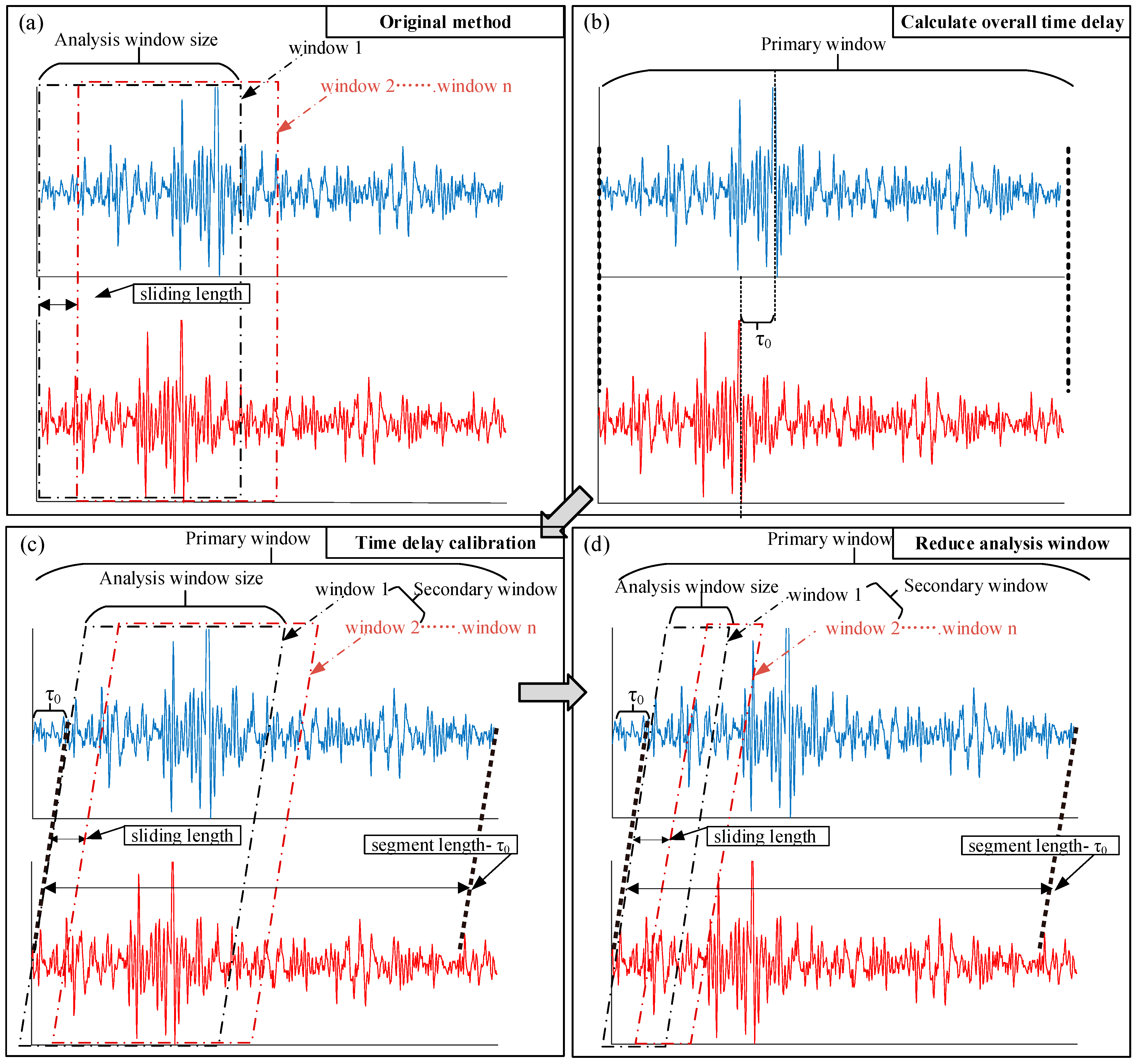
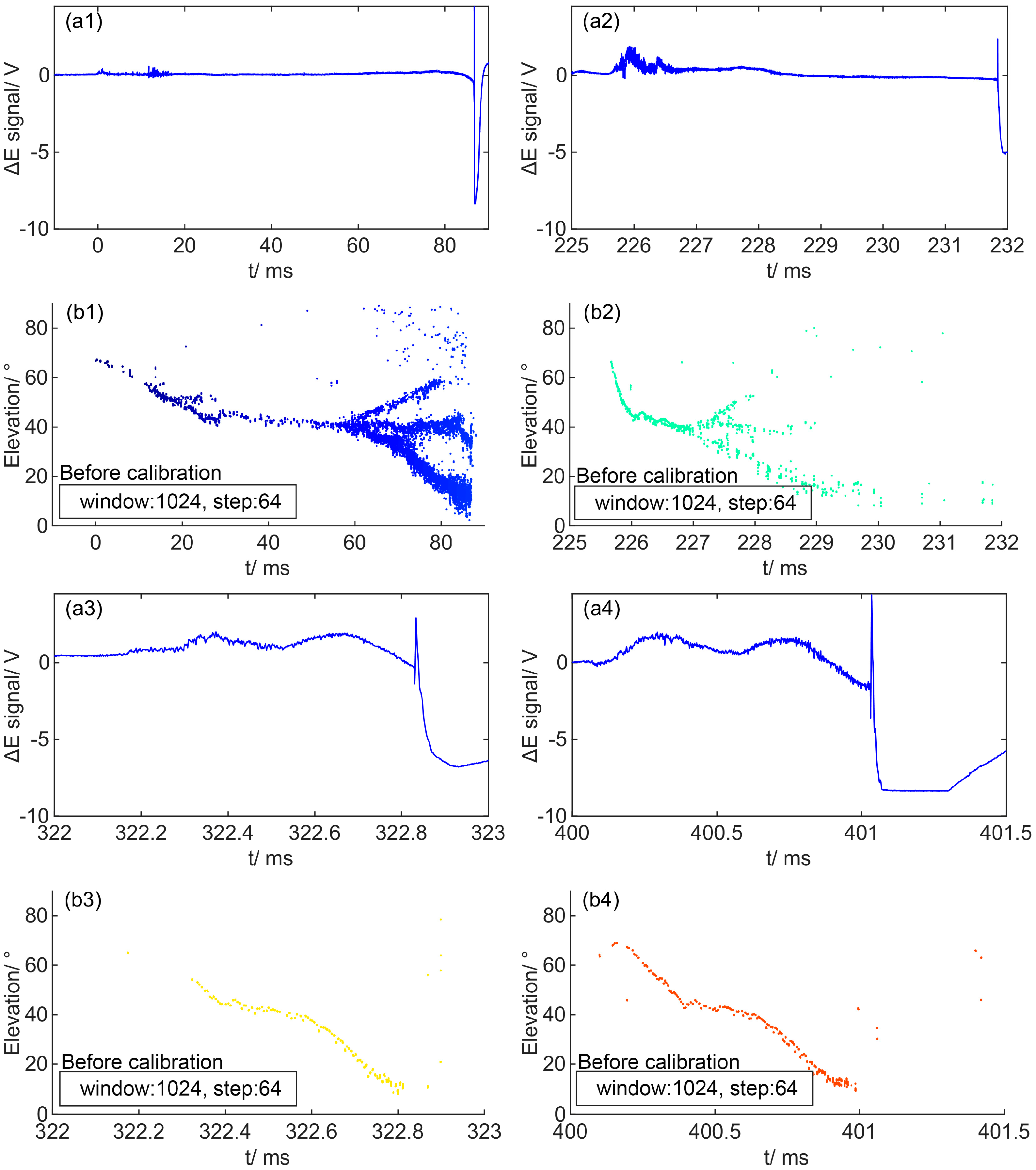
The use of the time delay calibration method can solve the problem of increased noise in the location results and improve the location effect when the data analysis window length is reduced.
(2)
After using the time delay calibration method, the correlation coefficient obtained via cross-correlation calculation in the process of locating calculation is improved, that is, this method improves the consistency of signals in the analysis window, and makes the input signals of locating calculation more stable and reasonable, thus improving the quality of the output results.
(3)
The correlation coefficient obtained via cross-correlation calculation in the locating calculation process can be used for the quality control of the locating results.

Author Contributions

Conceptualization, D.W. and H.L.; methodology, H.L.; software, H.L.; validation, W.D., W.L., B.W., Q.Q., Y.M., L.C. and Y.G.; writing—original draft preparation, H.L.; writing—review and editing, D.W. All authors have read and agreed to the published version of the manuscript.

Funding

This research was funded by the National Natural Science Foundation of China (grant numbers 41875005, 42075088, and 42105085).

Data Availability Statement

The data used in this paper are available upon request from the corresponding author.

Acknowledgments

Thanks to the editors and reviewers for their hard work and valuable advice.

Conflicts of Interest

The authors declare no conflict of interest.

References

  1. Rison, W.; Thomas, R.J.; Krehbiel, P.R.; Hamlin, T.; Harlin, J. A GPS-based three-dimensional lightning mapping system: Initial observations in central New Mexico. Geophys. Res. Lett. 1999, 26, 3573–3576. [Google Scholar] [CrossRef]
  2. Thomas, R.J.; Krehbiel, P.R.; Rison, W.; Hunyady, S.J.; Winn, W.P.; Hamlin, T.; Harlin, J. Accuracy of the Lightning Mapping Array. J. Geophys. Res. Atmos. 2004, 109, D14207. [Google Scholar] [CrossRef]
  3. Rhodes, C.T.; Shao, X.M.; Krehbiel, P.R.; Thomas, R.J.; Hayenga, C.O. Observations of lightning phenomena using radio interferometry. J. Geophys. Res. Atmos. 1994, 99, 13059–13082. [Google Scholar] [CrossRef]
  4. Liu, H.; Dong, W.; Wu, T.; Zheng, D.; Zhang, Y. Observation of compact intracloud discharges using VHF broadband interferometers. J. Geophys. Res. Atmos. 2012, 117, D1203. [Google Scholar] [CrossRef]
  5. Yoshihashi, S.; Kawasaki, I.; Matsuura, K.; Isoda, H.; Sonoi, Y. 3D imaging of lightning channel and leader progression velocity. Electr. Eng. Jpn. 2001, 137, 22–28. [Google Scholar] [CrossRef]
  6. Liu, H.; Qiu, S.; Dong, W. The Three-Dimensional Locating of VHF Broadband Lightning Interferometers. Atmosphere 2018, 9, 317. [Google Scholar] [CrossRef]
  7. Sun, Z.; Qie, X.; Liu, M.; Jiang, R.; Zhang, H. Three-Dimensional Mapping on Lightning Discharge Processes Using Two VHF Broadband Interferometers. Remote Sens. 2022, 14, 6378. [Google Scholar] [CrossRef]
  8. Hare, B.M.; Scholten, O.; Dwyer, J.; Trinh, T.N.G.; Buitink, S.; ter Veen, S.; Bonardi, A.; Corstanje, A.; Falcke, H.; Hörandel, J.R.; et al. Needle-like structures discovered on positively charged lightning branches. Nature 2019, 568, 360–363. [Google Scholar] [CrossRef]
  9. Scholten, O.; Hare, B.M.; Dwyer, J.; Liu, N.; Sterpka, C.; Kolmasov, I.; Santolik, O.; Lan, R.; Uhlir, L.; Buitink, S. Interferometric imaging of Intensely Radiating Negative Leaders. Phys. Rev. D 2022, 105, 062007. [Google Scholar] [CrossRef]
  10. Scholten, O.; Hare, B.M.; Dwyer, J.; Sterpka, C.; Kolmašová, I.; Santolík, O.; Lán, R.; Uhlíř, L.; Buitink, S.; Corstanje, A.; et al. The Initial Stage of Cloud Lightning Imaged in High-Resolution. JGR Atmos. 2021, 126, e2020JD033126. [Google Scholar] [CrossRef]
  11. Shao, X.M.; Krehbiel, P.R. The spatial and temporal development of intracloud lightning. J. Geophys. Res. Atmos. 1996, 101, 26641–26668. [Google Scholar] [CrossRef]
  12. Ushio, T.; Kawasaki, Z.I.; Ohta, Y.; Matsuura, K. Broad Band Interferometric Measurement of Rocket Triggered Lightning in Japan. Geophys. Res. Lett. 1997, 24, 2769–2772. [Google Scholar] [CrossRef]
  13. Shao, X.M.; Holden, D.N.; Rhodes, C.T. Broad Band Radio Interferometry for Lightning Observations. Geophys. Res. Lett. 1996, 23, 1917–1920. [Google Scholar] [CrossRef]
  14. Kawasaki, Z.; Mardiana, R.; Ushio, T. Broadband and Narrowband RF Interferometers for Lightning Observations. Geophys. Res. Lett. 2000, 27, 3189–3192. [Google Scholar] [CrossRef]
  15. Dong, W.; Liu, X.; Yu, Y.; Zhang, Y. Broadband interferometer observations of a triggered lightning. Chin. Sci. Bull. 2001, 46, 1561–1565. [Google Scholar] [CrossRef]
  16. Zhang, G.; Zhao, Y.; Qie, X.; Zhang, T.; Wang, Y.; Chen, C. Observation and study on the whole process of cloud-to-ground lightning using narrowband radio interferometer. Sci. China Ser. D-Earth Sci. 2008, 51, 694–708. [Google Scholar] [CrossRef]
  17. Li, Y.; Qiu, S.; Shi, L.; Huang, Z.; Wang, T.; Duan, Y. Three-Dimensional Reconstruction of Cloud-to-Ground Lightning Using High-Speed Video and VHF Broadband Interferometer. J. Geophys. Res. Atmos. 2017, 122, 13, 413–420, 435. [Google Scholar] [CrossRef]
  18. Yoshida, S.; Biagi, C.J.; Rakov, V.A.; Hill, J.D.; Stapleton, M.V.; Jordan, D.M.; Uman, M.A.; Morimoto, T.; Ushio, T.; Kawasaki, Z.I. Three-dimensional imaging of upward positive leaders in triggered lightning using VHF broadband digital interferometers. Geophys. Res. Lett. 2010, 37, L5805. [Google Scholar] [CrossRef]
  19. Jensen, D.P.; Sonnenfeld, R.G.; Stanley, M.A.; Edens, H.E.; Da Silva, C.L.; Krehbiel, P.R. Dart-Leader and K-Leader Velocity From Initiation Site to Termination Time-Resolved with 3D Interferometry. Geophys. Res. Atmos. 2021, 126, e2020JD034309. [Google Scholar] [CrossRef]
  20. Stock, M.G.; Akita, M.; Krehbiel, P.R.; Rison, W.; Edens, H.E.; Kawasaki, Z.; Stanley, M.A. Continuous broadband digital interferometry of lightning using a generalized cross-correlation algorithm. J. Geophys. Res. Atmos. 2014, 119, 3134–3165. [Google Scholar] [CrossRef]
  21. Lyu, F.; Cummer, S.A.; Qin, Z.; Chen, M. Lightning Initiation Processes Imaged With Very High Frequency Broadband Interferometry. J. Geophys. Res. Atmos. 2019, 124, 2994–3004. [Google Scholar] [CrossRef]
  22. Pu, Y.; Cummer, S.A. Needles and Lightning Leader Dynamics Imaged with 100–200 MHz Broadband VHF Interferometry. Geophys. Res. Lett. 2019, 46, 13556–13563. [Google Scholar] [CrossRef]
  23. Qiu, S.; Zhou, B.H.; Shi, L.H.; Dong, W.S.; Zhang, Y.J.; Gao, T.C. An improved method for broadband interferometric lightning location using wavelet transforms. J. Geophys. Res. 2009, 114, D18211. [Google Scholar] [CrossRef]
  24. Mardiana, R.; Kawasaki, Z.I. Dependency of VHF Broad Band Lightning Source Mapping on Fourier Spectra. Geophys. Res. Lett. 2000, 27, 2917–2920. [Google Scholar] [CrossRef]
  25. Shi, Q.; Bo, Y.; Wansheng, D.; Taichang, G. Application of correlation time delay estimation in broadband interferometer for lightning detection. Sci. Meteorol. Sin. 2009, 29, 92–96. [Google Scholar]
  26. Sun, Z.; Qie, X.; Liu, M.; Cao, D.; Wang, D. Lightning VHF radiation location system based on short-baseline TDOA technique—Validation in rocket-triggered lightning. Atmos. Res. 2013, 129–130, 58–66. [Google Scholar] [CrossRef]
  27. Akita, M.; Stock, M.; Kawasaki, Z.; Krehbiel, P.; Rison, W.; Stanley, M. Data processing procedure using distribution of slopes of phase differences for broadband VHF interferometer. J. Geophys. Res. Atmos. 2014, 119, 6085–6104. [Google Scholar] [CrossRef]
  28. Stock, M.; Krehbiel, P. Multiple baseline lightning interferometry—Improving the detection of low amplitude VHF sources. In Proceedings of the International conference on Lightning Protection, Shanghai, China, 11–18 October 2014; pp. 293–300. [Google Scholar]
  29. Wang, T.; Qiu, S.; Shi, L.; Li, Y. Broadband VHF Localization of Lightning Radiation Sources by EMTR. IEEE Trans. Electromagn. Compat. 2017, 59, 1949–1957. [Google Scholar] [CrossRef]
  30. Wang, T.; Shi, L.; Qiu, S.; Sun, Z.; Duan, Y. Continuous broadband lightning VHF mapping array using MUSIC algorithm. Atmos. Res. 2020, 231, 104647. [Google Scholar] [CrossRef]
  31. Li, S.L.; Qiu, S.; Shi, L.H.; Li, Y.; Duan, Y.T. Broadband very high frequency localization of lightning radiation sources based on orthogonal propagator method. Acta Physica Sin. 2019, 68, 279–287. [Google Scholar] [CrossRef]
  32. Li, F.; Sun, Z.; Liu, M.; Yuan, S.; Wei, L.; Sun, C.; Lyu, H.; Zhu, K.; Tang, G. A New Hybrid Algorithm to Image Lightning Channels Combining the Time Difference of Arrival Technique and Electromagnetic Time Reversal Technique. Remote Sens. 2021, 13, 4658. [Google Scholar] [CrossRef]
  33. Shao, X.M.; Ho, C.; Bowers, G.; Blaine, W.; Dingus, B. Lightning Interferometry Uncertainty, Beam Steering Interferometry, and Evidence of Lightning Being Ignited by a Cosmic Ray Shower. J. Geophys. Res. Atmos. 2020, 125, e2019JD032273. [Google Scholar] [CrossRef]
  34. Fan, X.P.; Zhang, Y.J.; Zheng, D.; Zhang, Y.; Lyu, W.T.; Liu, H.Y.; Xu, L.T. A New Method of Three-Dimensional Location for Low-frequency Electric Field Detection Array. J. Geophys. Res. Atmos. 2018, 123, 8792–8812. [Google Scholar] [CrossRef]
  35. Lyu, F.; Cummer, S.A.; Solanki, R.; Weinert, J.; McTague, L.; Katko, A.; Barrett, J.; Zigoneanu, L.; Xie, Y.; Wang, W. A low-frequency near-field interferometric-TOA 3-D Lightning Mapping Array. Geophys. Res. Lett. 2014, 41, 7777–7784. [Google Scholar] [CrossRef]
  36. Yang, J.; Wang, D.; Huang, H.; Wu, T.; Takagi, N.; Yamamoto, K. A 3D Interferometer-Type Lightning Mapping Array for Observation of Winter Lightning in Japan. Remote Sens. 2023, 15, 1923. [Google Scholar] [CrossRef]
Figure 1. Illustration of time delay calibration method: (a) the sliding window mode of the original method, (b) the first step of the time delay calibration method, (c) the window sliding mode of the time delay calibration method, and (d) same as (c) but for a reduced analysis window.
Remotesensing 15 02817 g001
Figure 2. Observation results of a negative CG flash at 15:40:06 on 13 June 2010: (a) fast electric field change signal, (b) elevation angle of radiation source with time, and (c) 2D location results of the elevation-azimuth angle. The locating calculation uses an analysis window of 1024 samples and slides every 64 sampling points. The color of the location points corresponds to their occurrence time.
Remotesensing 15 02817 g002
Figure 3. The observation results from Figure 2 are displayed in an enlarged view for the four stages of the discharge process: (a1,b1) show the process from the beginning of the lightning to the end of the first return stroke, (a2,b2) show the second leader process, (a3,b3) show the third leader process, and (a4,b4) show the fourth leader process.
Remotesensing 15 02817 g003
Figure 4. Comparison of locating results before and after using the time delay calibration method: (a) using an analysis window of 256 ns and a sliding window of 64 ns for calculation without the time delay calibration, (b) using an analysis window of 256 ns and a sliding window of 64 ns for calculation with the time delay calibration, (c) using an analysis window of 128 ns and a sliding window of 32 ns for calculation without the time delay calibration, and (d) using an analysis window of 128 ns and a sliding window of 32 ns for calculation with the time delay calibration.
Remotesensing 15 02817 g004
Figure 5. Statistical results of the residuals Rn and the average correlation coefficient (Coeff) corresponding to the results obtained using three groups of different analysis window lengths and sliding window lengths: (a,b) analysis window length of 1024 ns and sliding window length of 64 ns, (c,d) analysis window length of 256 ns and sliding window length of 64 ns, (e,f) analysis window length of 128 ns and sliding window length of 32 ns. The white color represents the results obtained using the original calculation method (marked as “O” in the legend), and the blue color represents the results obtained after time delay calibration (marked as “N” in the legend). In the panels (b,d,f), the white histogram has 40% transparency, and the blue histogram covered by it will reveal light blue.
Remotesensing 15 02817 g005
Figure 6. The 2D location results obtained using a 32ns analysis window and a 16ns sliding window are shown as (a) colored by occurrence time, (b) colored by the average correlation coefficient obtained during calculation, and (c) colored by the sum of signal amplitudes within each analysis window.
Remotesensing 15 02817 g006
Figure 7. The distribution relationship between the sum of signal amplitude in the analysis window and the average correlation coefficient of the localization results in Figure 6.
Remotesensing 15 02817 g007
Figure 8. Zoomed-in display similar to Figure 3, but using a 32 ns analysis window and a 16 ns sliding window, with localization points colored according to their corresponding average correlation coefficient. (a1a4) are same with the corresponding panels in Figure 3. (b1b4) show the same discharge stages as in the corresponding panels of Figure 3.
Remotesensing 15 02817 g008
Disclaimer/Publisher’s Note: The statements, opinions and data contained in all publications are solely those of the individual author(s) and contributor(s) and not of MDPI and/or the editor(s). MDPI and/or the editor(s) disclaim responsibility for any injury to people or property resulting from any ideas, methods, instructions or products referred to in the content.

