1. Introduction
In recent years, satellite remote sensing images have become increasingly utilized for monitoring land surface changes due to the continuous development of computer and space satellite technology. In particular, InSAR has emerged as a popular technology for monitoring surface subsidence changes, especially goaf deformation, as it is not impacted by weather and has extensive coverage [
1]. Goaf is formed after coal extraction from underground, and the continuous and efficient monitoring of surface subsidence above goaf can facilitate the understanding of surface subsidence damage to surface structures, explore mining subsidence mechanisms, and provide a decision-making basis for geological disaster prevention and ecological restoration in mining areas [
2]. The authors of [
3] estimated that the total economic losses due to subsidence from coal mining in China were approximately 32 billion CNY (about 4.9 billion USD) from 2001 to 2010. These losses were primarily due to damage to buildings, roads, and other infrastructure caused by surface subsidence above goaf. Surface subsidence caused by goaf formation can lead to accidents such as landslides, rockfalls, and collapses, which can result in injuries and fatalities; [
4] and [
5] reported that coal mining-related subsidence caused accidents, resulting in deaths or injuries every year in the world. Efficient monitoring of surface subsidence above goaf can help in preventing accidents and reducing economic losses [
6,
7,
8]. The traditional form of goaf surface subsidence monitoring involves point-like monitoring stations, which are characterized by high consumption, low efficiency, limited coverage, and insufficient monitoring capability. Thus, it is of immense theoretical value and practical significance to use the new monitoring method of goaf surface subsidence (InSAR) to explore the formation mechanism behind subsidence in key mining areas and predict the evolution law and development trend of subsidence based on new monitoring methods and technology. Recent advances in deep learning theory have had a significant impact on time series prediction. As a result, an increasing number of deep-learning algorithms are being utilized to research long time series prediction, thereby making it possible to obtain mine subsidence characteristic information and dynamic forecasting in mining areas [
9,
10]. Deep-learning algorithms such as artificial neural networks (ANNs) [
11] and recurrent neural networks (RNNs) [
12] can be used to analyze long time series data and predict mine subsidence characteristics and dynamics. However, these methods need further improvement to improve the accuracy of prediction.
InSAR, an active remote-sensing technology, has been widely used for monitoring subsidence and surface deformation [
13]. Initially, this technology was employed for ground elevation mapping [
14] and subsequently extended to surface deformation monitoring [
15]. However, the atmospheric phase delay and temporal and spatial decorrelation associated with two-pass InSAR technology can lead to phase unwrapping failure. Therefore, researchers proposed time series InSAR monitoring technology [
16], including PS-InSAR [
17] and SBAS-InSAR [
18], with the latter being more suitable for deformation monitoring in mining areas. SBAS-InSAR technology involves registering interferences in pairs of SAR data sets covering the same area and selecting interferograms whose temporal and spatial baselines meet the threshold [
19]. The highly coherent points in the images are then reconstructed based on the interferograms’ phase. SBAS-InSAR has shown high-quality monitoring results with sub-centimeter monitoring accuracy [
20,
21]. G. Herrera et al. [
22] demonstrated the monitoring capacity of InSAR technology using multi-sensor and multi-temporal SAR data in very slow landslides. Dario Peduto et al. [
23] used DInSAR technology to analyze building deformation and presented a multi-scale procedure tailored to analyze the settlement-induced building damage; it could forecast building damage in urban areas. M. P. Sanabria et al. [
24] proposed a methodology to produce subsidence activity maps based on PSInSAR data; these displacement map measurements are interpolated based on conditional Sequential Gaussian Simulation complement, and they are helpful for the identification of wide subsiding areas.
In the context of mining subsidence, InSAR technology has been increasingly recognized as a valuable tool for monitoring surface deformation. However, predicting subsidence movement remains a challenge and requires a prediction model that integrates InSAR data. To date, two broad categories of prediction models have been employed: traditional and late models. Traditional models use various technical methods to obtain surface deformation data post-mining and predict the maximum deformation value using mathematical functions or numerical models. Examples include numerical simulation, similar material simulation, probability integration, and other static prediction models [
25].
The mining subsidence process is a complex spatio-temporal phenomenon, posing challenges for applying static prediction models that cannot account for dynamic changes [
26]. Alternatively, continuous multi-period surface deformation data obtained by various technical means can be analyzed to predict the location and timing of maximum surface movement deformation by incorporating time functions such as Knothe [
27], Weibull [
28], and Logistic [
29]. However, these models can only capture the linear relationship between two vectors and are limited in their ability to predict nonlinear deformation in mining areas. Moreover, due to the dynamic changes in mining practices, such as mode, speed, and roof management, the accuracy of dynamic time function simulations is often compromised [
30]. Due to the complexity of the mining subsidence process in both time and space, static prediction models have limited practical application as they cannot simulate the dynamic changes in the subsidence process. In addition, the actual surface subsidence is different under different geological and mining conditions, but the prediction result is the same if the same time function is used, which is contradictory to the actual situation. Therefore, researchers have focused on “late models”, such as the grey model [
31], regression analysis [
32,
33], support vector machine regression [
9], Bayesian network [
10], wavelet analysis [
34], and artificial neural network [
35,
36]. These models rely on modern and efficient monitoring means such as GNSS, InSAR, and LIDAR to obtain long-term series monitoring data and analyze internal statistical laws and trends. However, these methods are sensitive to model parameters, and adding mining geological parameters for goaf prediction can be challenging.
Compared to traditional mining subsidence prediction methods and late models, deep learning offers a novel approach to address this challenge. By formulating the relationship between response variables in a regression equation, deep-learning algorithms can accurately capture the impact of independent variables influenced by one or more dependent variables. While previous deep-learning techniques such as BP neural networks [
37] and recurrent neural networks (RNN) [
12] have been developed, they have not been ideal for long-term series prediction [
38]. However, recent studies have shown that LSTM models, which combine RNN and attention mechanisms, are better suited for long-term prediction [
39]. These models use a cellular structure, with the forgetting gate discarding unnecessary information while the memory gate retains important information.
Homa Ansari et al. [
40] conducted an experiment on the Lazufre Volcanic Complex, situated in the central volcanic region, concluding that signal error associated with InSAR technology is a crucial factor contributing to inaccurate predictions when combined with LSTM. Hill et al. [
41] focused on the influence of seasonal perturbations on forecasting outcomes. The LSTM prediction methodology proved efficient for short-term projections (less than three months). Qinghao Liu et al. [
42] proposed a heterogeneous LSTM network model, which integrates spatial heterogeneity into predicting ground subsidence, successfully achieving accurate and efficient large-scale subsidence forecast. Yi Chen et al. [
43] demonstrated the effectiveness of an unimproved LSTM neural network approach for time-series InSAR land subsidence prediction. Despite using InSAR technology and LSTM network models to forecast deformation, these studies produce contradictory findings due to the insufficient recognition of the significance of the InSAR training data, particularly in areas affected by error signals, such as volcanic and mining regions. Above all, the traditional InSAR needs to be improved to monitor mine deformation; inaccurate training data do not help improve the prediction accuracy of deep learning [
44,
45]. The purpose of this study is to obtain fine subsidence characteristics and accurate data on mining surfaces by improving InSAR technology and realize the accurate prediction of mining surface subsidence combined with the LSTM algorithm. This study presents an integrated monitoring and prediction model for the goaf surface that combines SBMHCT-InSAR and LSTM algorithms. The utilization of SBMHCT-InSAR technology enhanced multiple aspects of image processing and interpretation, such as the image registration algorithm, interferogram filtering method, and high coherence point extraction method. The objective of these advancements is to mitigate the disruptive influence of noise signal and optimize the training data of the prediction model, ultimately resulting in an enhanced level of accuracy. In practice, this technology is leveraged in the monitoring of goaf surface deformation, facilitating the retrieval of settlement values from equal interval time series training data. Additionally, the LSTM algorithm is employed to establish a deformation prediction model for coal mining areas by drawing the global dependence relationship between input and output and learning the nonlinear patterns and features of the training data. The main aim of this research is to forecast geological hazards while also addressing practical problems associated with the prediction of goaf subsidence using InSAR technology with deep learning theory. The study findings not only offer methodological support for mining subsidence management but also promote the quantitative application and development of InSAR technology. Therefore, the proposed model carries significant scientific and practical value.
2. Materials and Methods
2.1. Site Selection
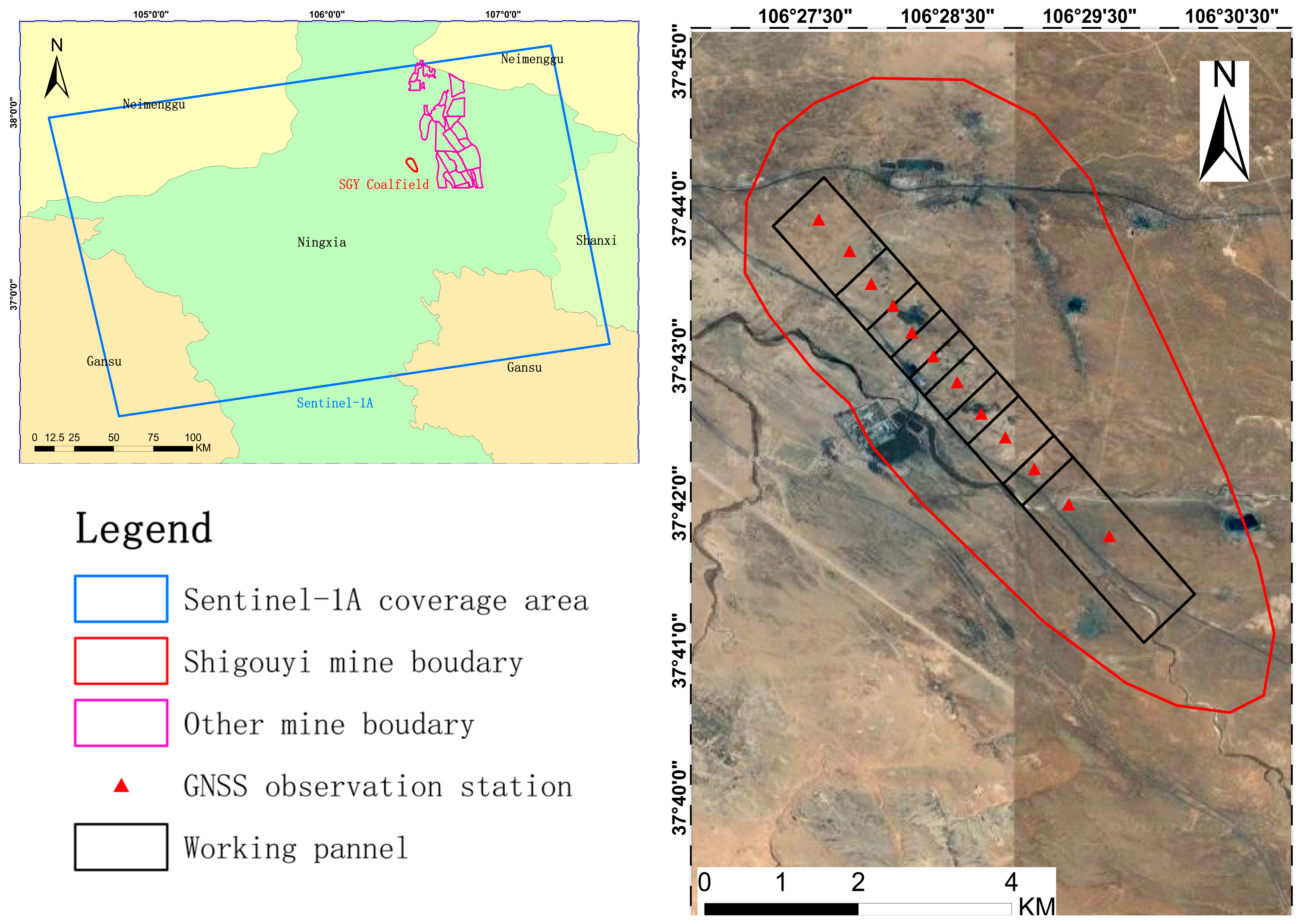
The Shigouyi (SGY) mine area, one of the Ningdong coalfields situated in the eastern region of the Ningxia province, is depicted in
Figure 1, with its geographical coordinates falling between 37°39′15″–37°45′17″N and 106°27′49″–106°30′44″E. It stretches westward to the Liupan Mount tectonic zone and eastward to the Erdos coal seam; it comprises a series of folds and faults. However, the Shigouyi mine experiences a significant, concentrated distribution of surface damage and subsidence because of its location on the Loess Plateau. The geological structure above the coal beds susceptible to mining is highly fragile.
Considering space constraints, this study focuses primarily on monitoring and predicting surface subsidence in the SGY coal mine. In this regard, a total of 13 GNSS observation stations have been installed above the working face of the mine, and the corresponding settlement data have been collected for verification of the experimental findings. The Chinese Southsurvey GNSS receivers were utilized to collect GNSS data in the real-time kinematic mode. One receiver was situated at the base station, which was positioned on a stable surface, while the others monitored displacements at the GNSS stations. The GNSS receiver exhibited horizontal and vertical accuracy of mm and mm (where D is the distance), respectively. Over the period of 9 March 2015 to 1 July 2016, GNSS-RTK measurements were taken at intervals of 24 days. Initially, a GNSS receiver with a tripod was installed on the reference station situated on the stable surface, where the antenna height was measured; receivers were opened; and the reference station height, antenna height, and WGS84 coordinate were inputted. The radio channel was then turned on and checked. The roving station GNSS receiver was subsequently opened with a centering rod, exact parameters were inputted, the radio channel and number of satellites were checked, and simultaneous observation with the reference station GNSS receiver was completed. Using the roving station GNSS receiver, the 12 GNSS stations’ coordinates and heights were measured. Data were obtained at a sampling rate of 20 Hz, with the observation time being more than 180 s. These 12 GNSS stations were measured again in the same manner at intervals of 24 days in the ensuing months, with the deformation value calculated by the difference value of these times, while quality control measures were taken each time. Verification of the reliability of the RTK results was conducted using the method of comparison with quick static measurement, where at least three points were selected as checkpoints, and the observation time of quick static measurement exceeded 600 s. After data processing, the maximum error between quick static measurement and RTK was less than 2 cm in height.
2.2. Data Selection
This study processed 19 SAR images (C-band) obtained from the Sentinel-1 satellite over a 15-month period from 9 March 2015 to 7 June 2016.
Table 1 shows the parameters of the SAR data used in this study; their temporal resolution is 24 days, and their spatial resolutions are 20 and 5 m in azimuth and range, respectively.
The SAR data cover a large area, including the SGY mine area, and due to computational efficiency, SAR data are clipped in pre-processed procedure. The European Space Agency (ESA) released precise orbit ephemerides (POD) data for all the Sentinel-1 SAR data. POD data are important for reducing registration errors. These data are used for phase re-flattening and orbital refinement. To eliminate the impact of topography on the measured surface deformation, the authors employed the three-arc-second Shuttle Radar Topography Mission (SRTM) Digital Elevation Model (DEM) obtained from the National Aeronautics and Space Administration (NASA).
2.3. Fundamental Principle of SBMHCT-InSAR Technique
The present study puts forward SBMHCT-InSAR technology for precise inversion of surface deformation. The proposed approach integrates the Permanent Scattering (PS) and high-coherence target methods. Linear and nonlinear deformation inversion methods are employed using the coherent target and singular value decomposition methods, respectively. SBMHCT-InSAR technology comprises key steps such as interference pair combination of multi-principal images, high-precision image registration, interferometric phase noise filtering, high-coherence target extraction, and the deformation inversion method. The SBMHCT-InSAR processing steps are as follows:
2.3.1. Group the SAR Pairs
There are 19 scenes of SAR images ordered at times (t
0,…, t
N) over the SGY mine area. M interferograms are constructed using installed multiple thresholds. The quantity
M is such that it adheres to the following inequality:
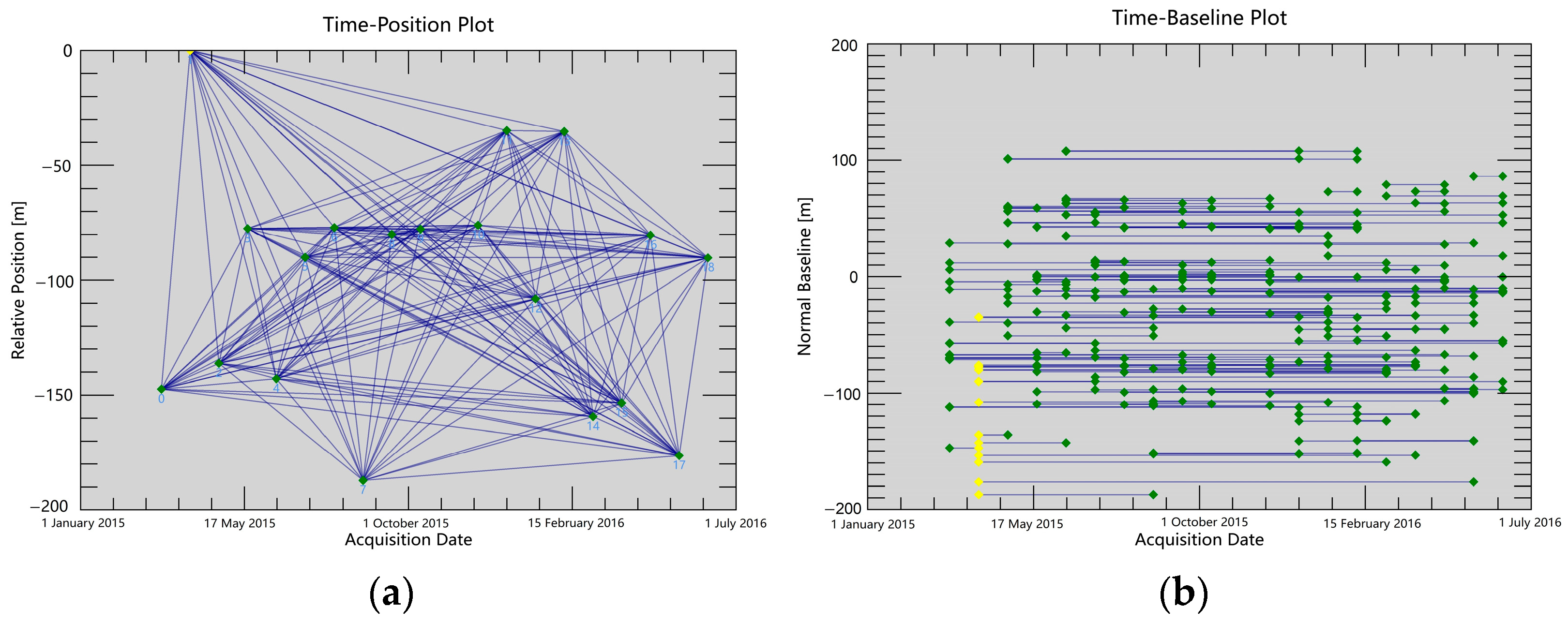
Figure 2 illustrates the experimental setup of the SAR pairs’ connection diagram. The experiment set thresholds of spatial and temporal baselines as 300 m and 200 days, respectively. The SAR data acquired on 2 April 2015 were selected as the super master image; others were co-registered and resampled. Other images that meet the threshold condition also generate interferometric pairs, resulting in 78 differential interferometric images.
2.3.2. Highly Accurate Image Registration
This paper presents an optimal matching point-based InSAR image registration method. Initially, an external DEM is emulated as a synthetic SAR image, and matching features are extracted from the SAR image to be registered in the simulated image. Then, the vector field consistent point set matching algorithm is employed to eliminate the homonymous feature points between the primary and secondary SAR images, remove the external points, and compute the polynomial transformation parameters for accurate registration. Ultimately, high-precision registration of the InSAR image is achieved.
2.3.3. Noise Filtering of Interferometric Phase
This study proposes an interferogram filtering method based on binary decomposition, which has the potential to effectively address the issue of noise in SAR images. The proposed approach decomposes the interferogram using a binary empirical mode algorithm into image and noise information. Filtering is then performed using a local window signal-to-noise ratio as the filtering factor, with strong filtering applied in regions of high noise and weak filtering in regions of low noise. Specifically, the method decomposes the original interferogram into fourth-order intrinsic mode function (IMF) signals and uses the signal-to-noise ratio of local windows as the filtering factor of the Goldstein filter to filter the first third-order IMF signals, which contain most of the noise information. The method demonstrates a strong noise-filtering ability while also preserving the edge details of interference fringes. As a result, the coherence of the interferogram is improved significantly after filtering.
2.3.4. High-Coherence Target Extraction
In 2004, Hooper [
46] introduced the StaMPS method, which identifies highly coherent points based on the stability of their phase values and high coherence and signal-to-noise ratio. Another method used to identify high-coherence points involves selecting a radius of a circle around known high-coherence points and then applying the amplitude dispersion threshold method to find candidate high-coherence points. Next, iterative analysis is carried out on the phase stability of the candidate points, and the high-coherence points are determined. This method reduces the computational workload and improves efficiency [
47].
2.3.5. Deformation Inversion
The proposed method aims to generate a Delaunay triangulation network for the highly coherent points after differential interferogram generation and identification of the highly coherent points. A linear model of velocity and elevation errors is then established based on the phase difference between two adjacent highly coherent points on the interferogram. By solving the coherence coefficient equation of the model, the incremental values of deformation velocity and elevation error are determined. The absolute value is obtained by incremental integration of the velocity and elevation error of several points. Next, the residual phase is unwrapped and calibrated by the discrete point phase after removing the linear model phase. Subsequently, the residual phase of a single SAR image is inverted using an interference combination matrix. Finally, nonlinear deformation and atmospheric influence phases are separated through time and space filtering, and a time series deformation sequence is obtained by calculating the linear deformation rate and nonlinear deformation phase.
Above all, the SBMHCT-InSAR technology introduced above is improved on the basis of SBAS-InSAR technology. Interactive Data Language (IDL) used for programming to improve the key steps of SBAS-InSAR technology, including image registration, filtering, and high coherence point extraction, in order to improve the adaptability and accuracy of SBAS-InSAR technology in mining deformation application.
2.4. Principles of LSTM
The LSTM network introduces a gate mechanism in the hidden layer to regulate information loss and dynamically adjusts the backpropagation process, enabling the network to learn long-distance time series data. This mechanism is crucial for the successful application of the LSTM model in large-scale surface subsidence prediction over extended time periods.
2.4.1. The Framework of LSTM
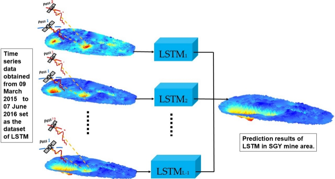
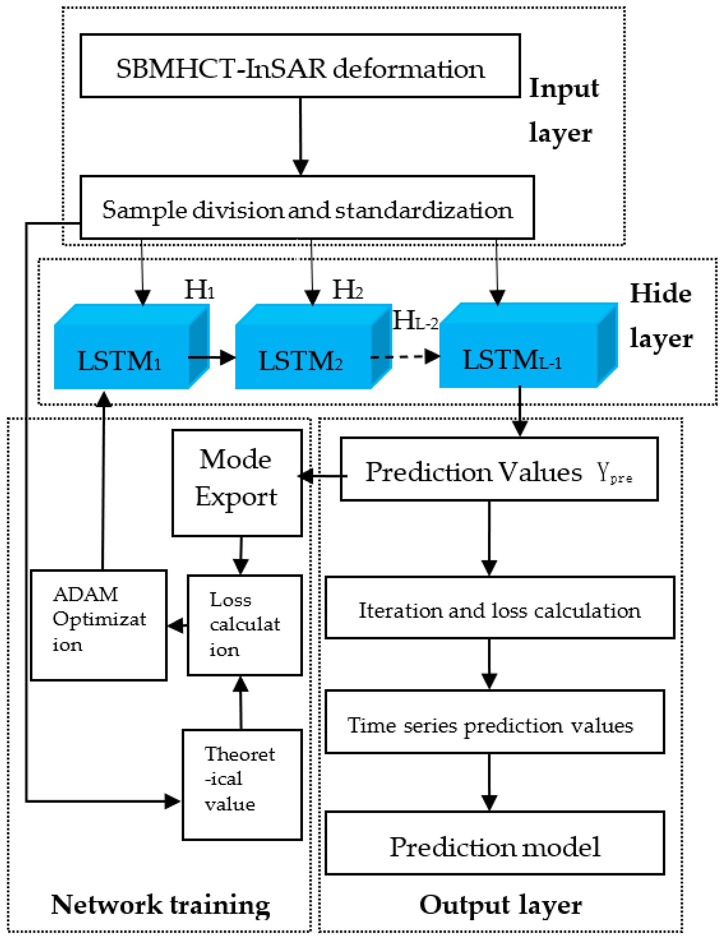
Figure 3 illustrates the prediction framework for time series mine subsidence based on LSTM. The original settlement data are pre-processed to meet the network input requirements in the first step, while the hidden layer uses the cell structure to construct the circulating neural network. Then, predicted values are exported by the output layer. The network training calculates the loss value between the predicted and true values and uses the ADAM algorithm to optimize the model. By dynamically adjusting the long and short-term memory network, the network can fully learn the nonlinear correlation of different subsidence time series and thus capture the complex subsidence mechanism in the study area. This approach not only reduces the requirement for high-quality diachronic data but also improves the accuracy and interpretability of subsidence prediction.
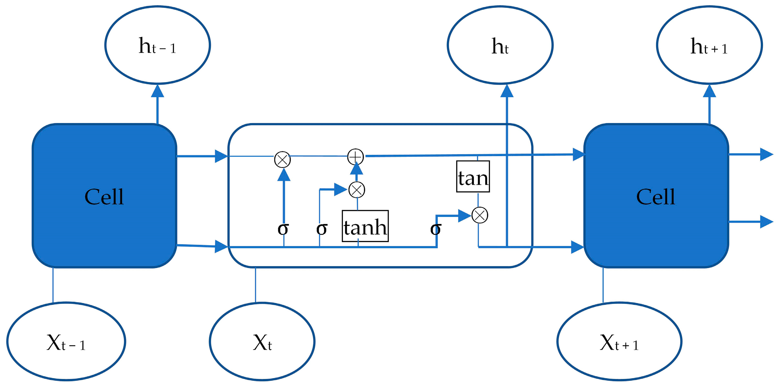
2.4.2. Cell Structure of LSTM
The LSTM network comprises a set of cell units that serve as the central structure in the hidden layer.
Figure 4 illustrates that the hidden layer contains three cell units. In the LSTM model, the input data at time t in the sample time series are represented by
, while the corresponding output data of the cell unit in the implicit state are represented by
. The flow of data in each cell unit is executed sequentially for input, information forgetting, cell state update, and implicit state output. The forward calculation method can be expressed as follows:
where
,
f,
c, and
o represent the input gate, forgetting gate, cell state, and output gate, respectively;
W and
b represent the corresponding weight coefficient matrix and bias, respectively;
and
refer to the sigmoid and the hyperbolic tangent activation function, respectively.
The training process of the LSTM network adopts time backpropagation (BPTT), which is similar to the traditional backpropagation algorithm [
48]. The algorithm involves four steps: First, the output of the cells is calculated based on the forward-computation method specified in Equation (5). The error term for each cell is then calculated in reverse, including time and network level backpropagation. Then, the gradient of each weight is determined according to the corresponding error term. Finally, the weights are updated using a gradient optimization algorithm.
2.5. Time Series Prediction Model Combining SBMHCT-InSAR Results and LSTM
Drawing on the fundamental tenets of the LSTM algorithm, the time series of coal mine subsidence obtained via InSAR technology are leveraged as training samples. Notably, these data exhibit nonlinear relationships, taking the form of . As such, the values of these data serve as the training samples for the LSTM algorithm, whereby a predictive model is established, the model parameters are solved, and the corresponding predicted values are obtained. The accuracy of the predictive model is evaluated by comparing the expected value with the corresponding truth value. Ultimately, the mine forecasting method is implemented in Python language.
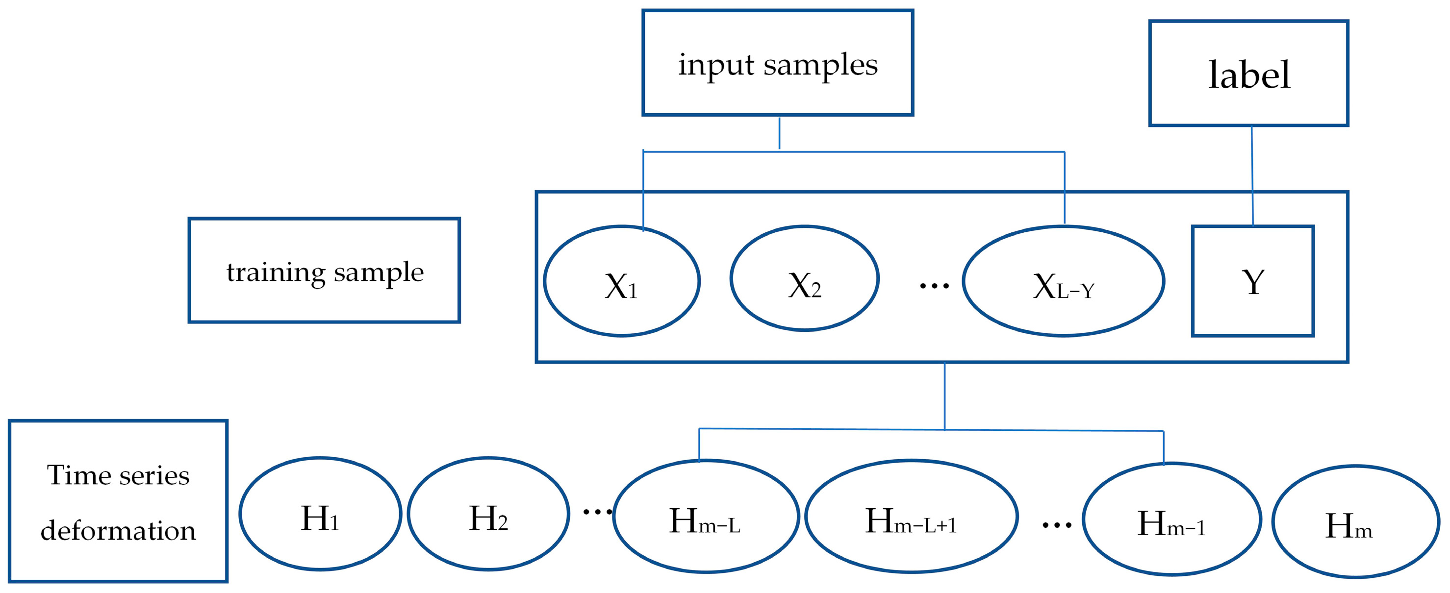
Step 1: Data pretreatments. The settlement time sequence data are processed by extracting a training sample of length L, denoted as
, from which the last Y values are designated as sample labels, and the first (L−Y) values are used as sample inputs, subject to the constraints of 2 ≤ L < m and 1 ≤ Y < L.
Figure 5 depicts the form of sample division. By implementing this segmentation method, all highly coherent target points are pre-processed, and
n training samples can be extracted. The paper adopts a single-step prediction method to construct the network model, whereby the length of the output sequence Y is set to y, and the settlement at the L moment is predicted based on the settlement information at the first (L−Y) moment.
Step 2: Network training. In
Figure 3, the hidden layer output value
is the final output through all LSTM hidden layer cell units. The input sample
of the hidden layer is a two-dimensional array; output
of the hidden layer and sample label
are both one-dimensional arrays (
n,1), where
n represents the number of highly coherent points. In this paper, the statistical error index is the mean square error, and the following formula is defined as the loss function of the training process:
Step 3: Parameter optimization. To construct an accurate LSTM prediction model, several parameters need to be considered, including the sample partition length (
L), network layer number (
K), and feature number (
S) of each LSTM hidden layer [
49,
50]. This paper employs a multi-layer grid search method to explore these parameters and selects the parameter combination with the highest average prediction accuracy as the optimal choice. The accuracy is determined by minimizing the prediction error (
ε) between the predicted sample (
Ypre) and the actual sample (
Y). The objective function is expressed as follows:
where STEP
L, STEP
K, and STEP
S are the grid search STEP
S of corresponding parameters, respectively.
Step 4: Output and accuracy assessment. The LSTM model can adapt the parameters during the training and validation process simultaneously, leading to the attainment of the optimal model . This model is then used to predict the future settlement amounts by inputting all standardized prediction samples in a sequential manner. The output of the model is represented as , where denotes the set of prediction results of different highly coherent points. Finally, the discrepancy between the output and the actual measured data in the course of deep learning prediction is computed, thereby providing a quantitative assessment of the training and prediction accuracy of the model.
Above all, the LSTM neural network was built based on Python 3.9 language and the Pytorch 1.10 deep learning framework [
43]. The input dataset includes all highly coherent point feature vectors obtained by SBMHCT-InSAR technology, containing longitude, latitude, coherence value, cumulative time, deformation rate, and cumulative subsidence value, among which cumulative subsidence value is the label data predicted in the model. The grid search algorithm was applied to select the hyperparameters in the LSTM ground deformation prediction model.
The absolute errors (AE) and the relative error (RE) are defined as follows:
where
represents the truth value and
represents the predicted value obtained by the LSTM model, and the absolute value is taken to avoid negative errors. The absolute error reflects the magnitude of the errors between the predicted and truth values, while the relative error indicates the proportion of the error relative to the truth value.
The relative error of the predicted results was evaluated using the Mean Absolute Percentage Error (MAPE). The generalization performance and degree of error of the prediction model were evaluated using the Wilmot Consistency Index (WIA), with values ranging from 0 to 1. Specifically, the MAPE was defined as the average of the absolute difference between the predicted and truth values, normalized by the observed value, expressed as a percentage. On the other hand, WIA was defined as the ratio of the observed variance to the sum of the observed variance and the variance of the prediction residuals, which were used to measure the degree of deviation of the model from the true values. They are defined as follows:
where
represents the truth value,
represents the predicted value obtained by the LSTM model,
n is the number of samples, and
is the average of
.
3. Results and Discussion
3.1. Analysis of InSAR Results
In order to confirm the precision and dependability of our experimental results, we conducted an analysis and comparison of InSAR data and the GNSS values in the SGY mining area. As discussed in [
51], the study area’s InSAR monitoring and precision verification outcomes have been documented and will not be reiterated here.
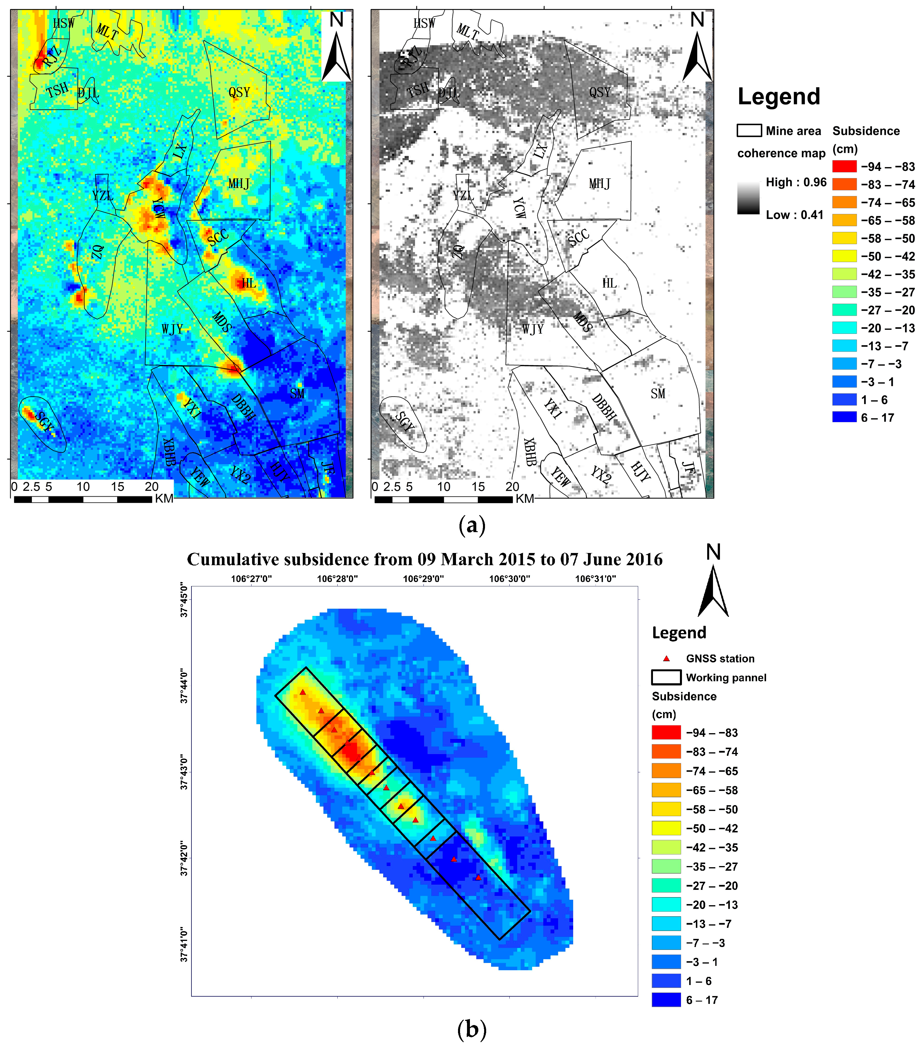
Figure 6a shows the cumulative deformation and coherence maps in the Ningdong coalfield; the graphs show a broader area to exhibit the mesoscale results, and the SGY mine is located in an oval area in the southwest. The coherence diagram shows that the coherence of the interferogram is greater than 0.41, and the coherence is good.
Figure 6b shows the cumulative deformation maps in the SGY mining area from March 2015 to June 2016, where the red triangle represents the GNSS observation stations and the black rectangles represent the location of the underground coal seam. Here, a total of 4795 pixels obtained deformation values from InSAR data; these values were calculated by dividing by the cosine of the incident angle to obtain the vertical deformations.
Based on this research, a significant deformation basin has emerged in the study area since March 2015, which is caused by the continuous mining activities in the study area. The maximum observed deformation in the mining area was as high as −94 cm, which is a typical example of the subsidence basin commonly observed during the excavation and mining activities in this area.
The InSAR monitoring of accumulated deformation value error within the study area satisfies standard specifications, validating the applicability of this research outcome for settlement prediction. In contrast to GNSS scattered point deformation monitoring with time series values, InSAR technology acquires continuous and planar deformation information, which can be utilized to predict surface subsidence and provide an effective representation of both the evolving surface trends and the regional distribution of subsidence.
3.2. LSTM Prediction Results
In the present study, 15 sets of InSAR monitoring data obtained between 9 March 2015 and 27 March 2016 were utilized as training samples, while 3 sets of InSAR monitoring data obtained between 27 March 2016 and 7 June 2016 were employed as test samples. Following the deformation results, the settlement sequence of each observation point was pre-processed, and 12 observation points were selected for further analysis.
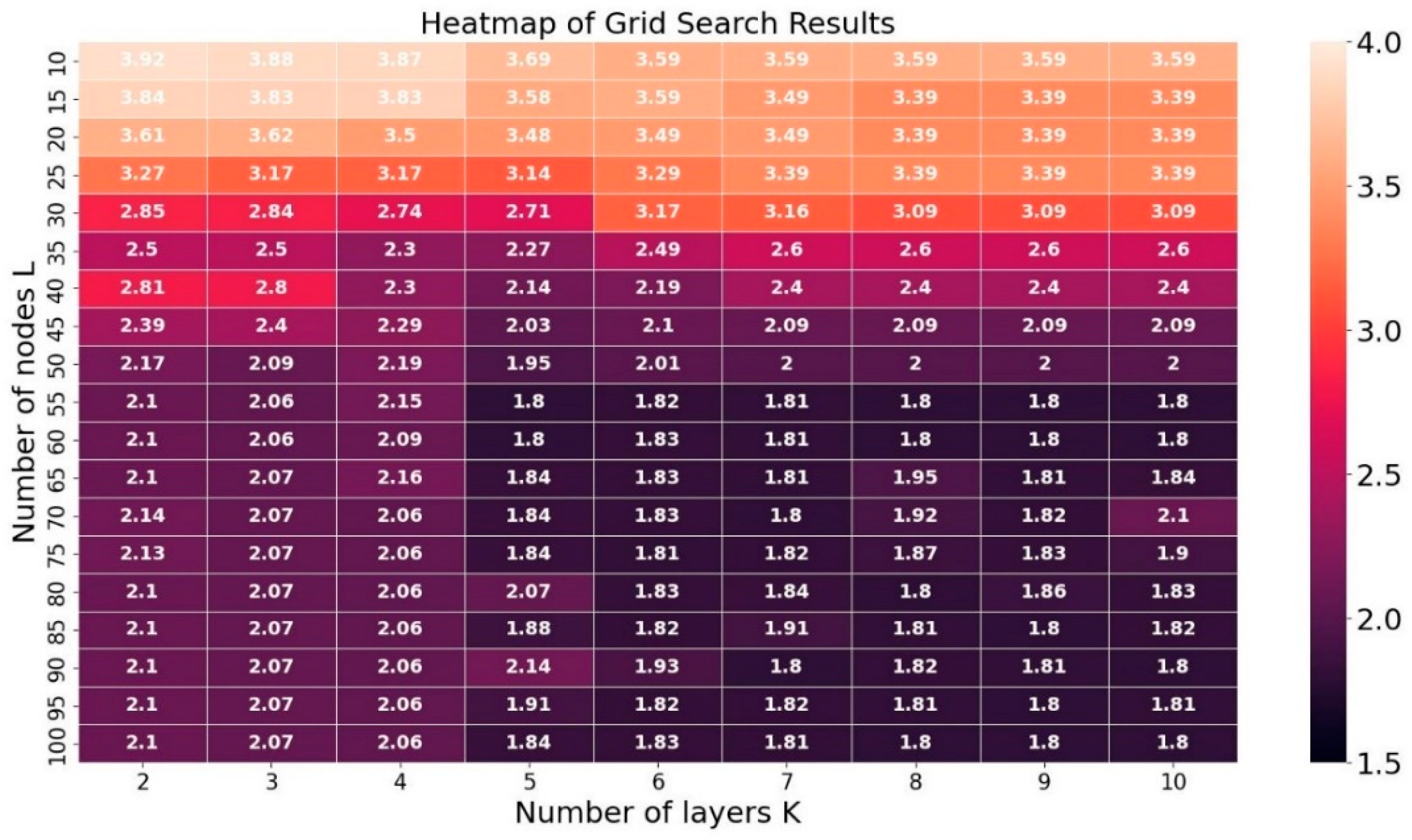
In this study, the settlement time sequence of each observation point was pre-processed based on the inversion results, and a total of 4795 points were selected as training samples. To determine the optimal network parameters, a grid search method was utilized to investigate the impact of the number of network layers
K and the number of hidden layer nodes
S on the prediction accuracy. The resulting heatmap of prediction errors, shown in
Figure 7, reveals that the number of network layers and hidden layer nodes are not solely responsible for prediction accuracy. While increasing the number of network layers generally enhances the prediction accuracy, and increasing the number of hidden nodes generally does the same, these correlations are not absolute. The prediction error reaches a trough when the number of network layers
K reaches 5, and the number of hidden nodes
S reaches 55. Further increasing the number of network layers and hidden nodes results in decreased efficiency of the prediction model without improving the prediction accuracy. Therefore, the optimal configuration for this study’s LSTM network consists of 5 layers and 55 hidden layer nodes.
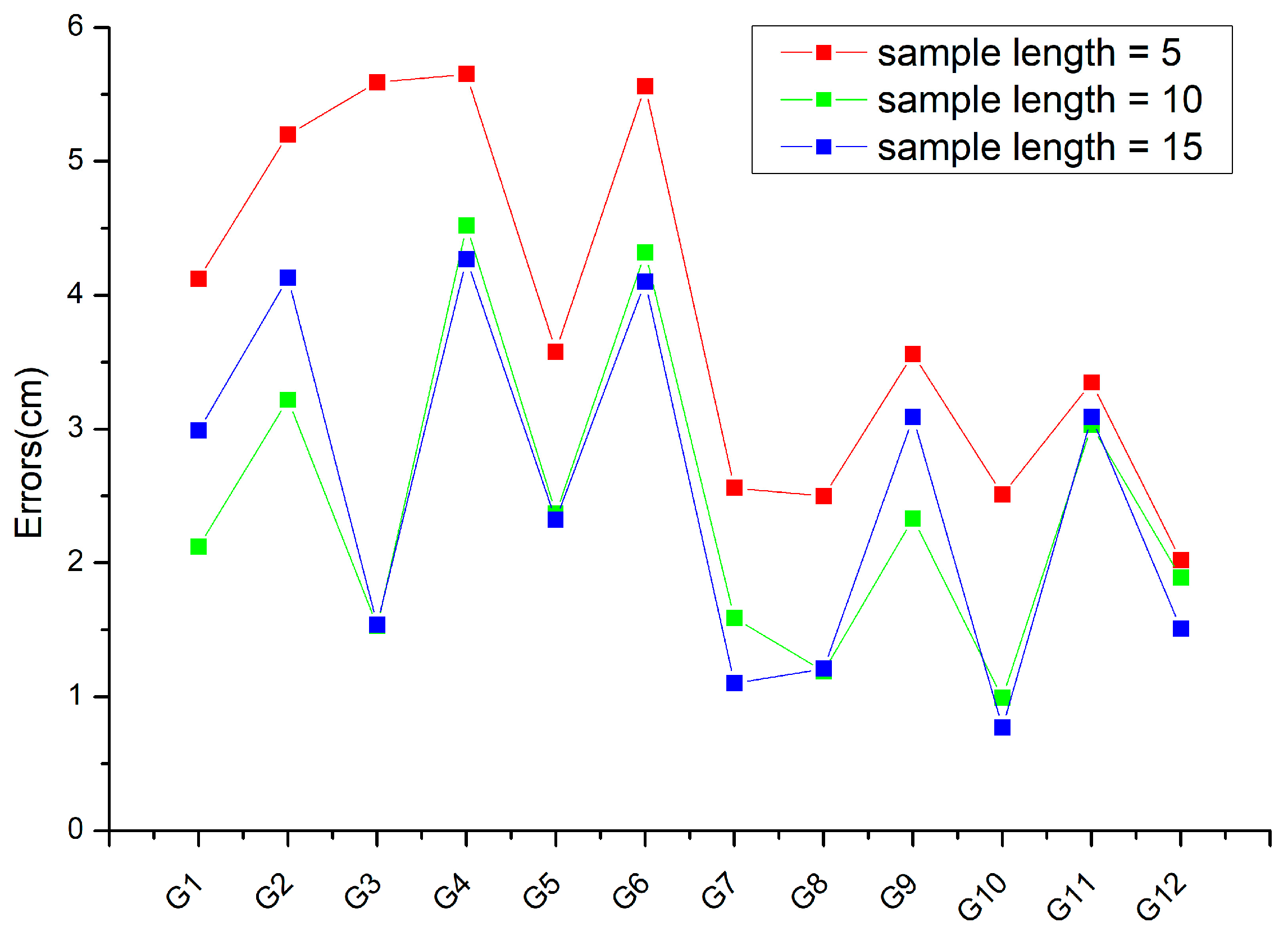
The focus of this study is on the 12 observation stations located in the center of the subsidence area. The objective is to investigate the relationship between the length of training samples and the prediction error. Additionally, the performance of each observation point in both single-step prediction and multi-step prediction is evaluated.
Figure 8 presents a line chart depicting the relationship between the length of training samples and the average prediction error. The predicted step is set as a single-step prediction. The 12 observation stations located in the center of the subsidence area are analyzed in this study to understand the error performance of each observation point. The results indicate that when the training sample length is 5, the prediction errors for all points are considerably higher compared to the prediction results of others. However, when the training sample length is set to 10, some observation points, such as G1, G2, and G9, exhibit better prediction results, while others show larger or similar errors with the prediction results of the blue line. The reason for this could be the fluctuation in subsidence values at these points. On the other hand, when the training sample length is set as 15, the prediction errors for all observation points are significantly lower. The line chart highlights that increasing the number of training samples results in lower prediction errors. Moreover, the local minimum prediction error of grid search gradually decreases with the increase in training sample length. Overall, the LSTM model performs better in predicting settlement values that exhibit stable and orderly changes over a longer period.
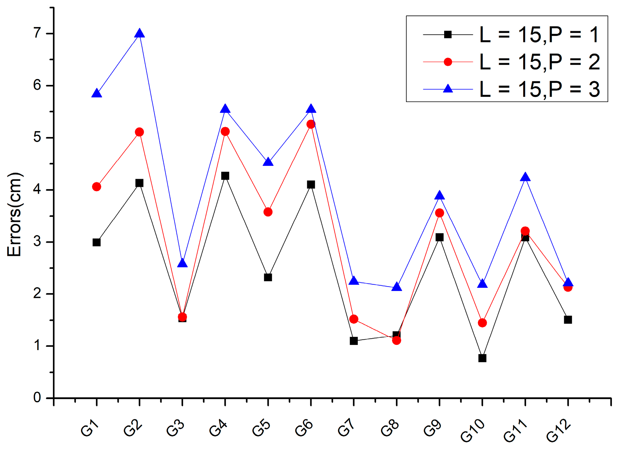
Figure 9 presents a line chart depicting the relationship between the predicted step size and the average prediction error. Based on the analysis, it can be observed that the prediction error increases with the increase in the predicted step size. This is because the longer the prediction sequence, the greater the cumulative error, resulting in a larger error in the predicted values. The error value of the light blue curve, which represents the predicted value error when the predicted step size is 3, is the largest among the three curves, indicating that the error accumulates with the increase in the predicted step size. The red curve and the dark blue curve have similar error values, indicating that the error accumulation is relatively small for multi-step prediction with a predicted step size of 2, and the prediction accuracy is still relatively high. However, it is worth noting that for some observation points with small cumulative form variables, the single-step prediction error is slightly smaller than that of multi-step prediction, which may be related to the characteristics of the subsidence process at these points. Overall, single-step prediction is a more accurate and reliable prediction method for SBMHCT-InSAR deformation monitoring values based on the LSTM model.
In multi-step prediction, the model needs to predict several time steps ahead, which increases the complexity of the problem. As a result, the prediction error may accumulate over time, leading to a less-accurate prediction. On the other hand, in single-step prediction, the model only needs to predict the next time step, which is a simpler problem, and therefore the average error is better than that of multi-step prediction.
The present study adopts a strategic approach for selecting the sample segmentation length by leveraging the outcomes of the experiments conducted. Specifically, given the small ordinal number and equal time interval of the data, and taking into consideration the LSTM model’s ability to learn long-distance time-series data, longer sample lengths were preferred to achieve better prediction results. In this regard, 15 sets of InSAR monitoring data obtained from 9 March 2015 to 27 March 2016 were selected as the training samples, whereas 3 sets of InSAR monitoring data from 27 March 2016 to 7 June 2016 were chosen as the test samples. The table below presents the final combination of LSTM prediction model parameters.
Table 2 shows the parameters of LSTM. Under the aforementioned parameter configuration, the experiment predicting surface subsidence in the SGY coal mine has yielded favorable results. Specifically, the average absolute difference (cumulative) form variable error has been effectively constrained to within 3 cm, thereby satisfying the accuracy standards prescribed within current InSAR data processing protocols.
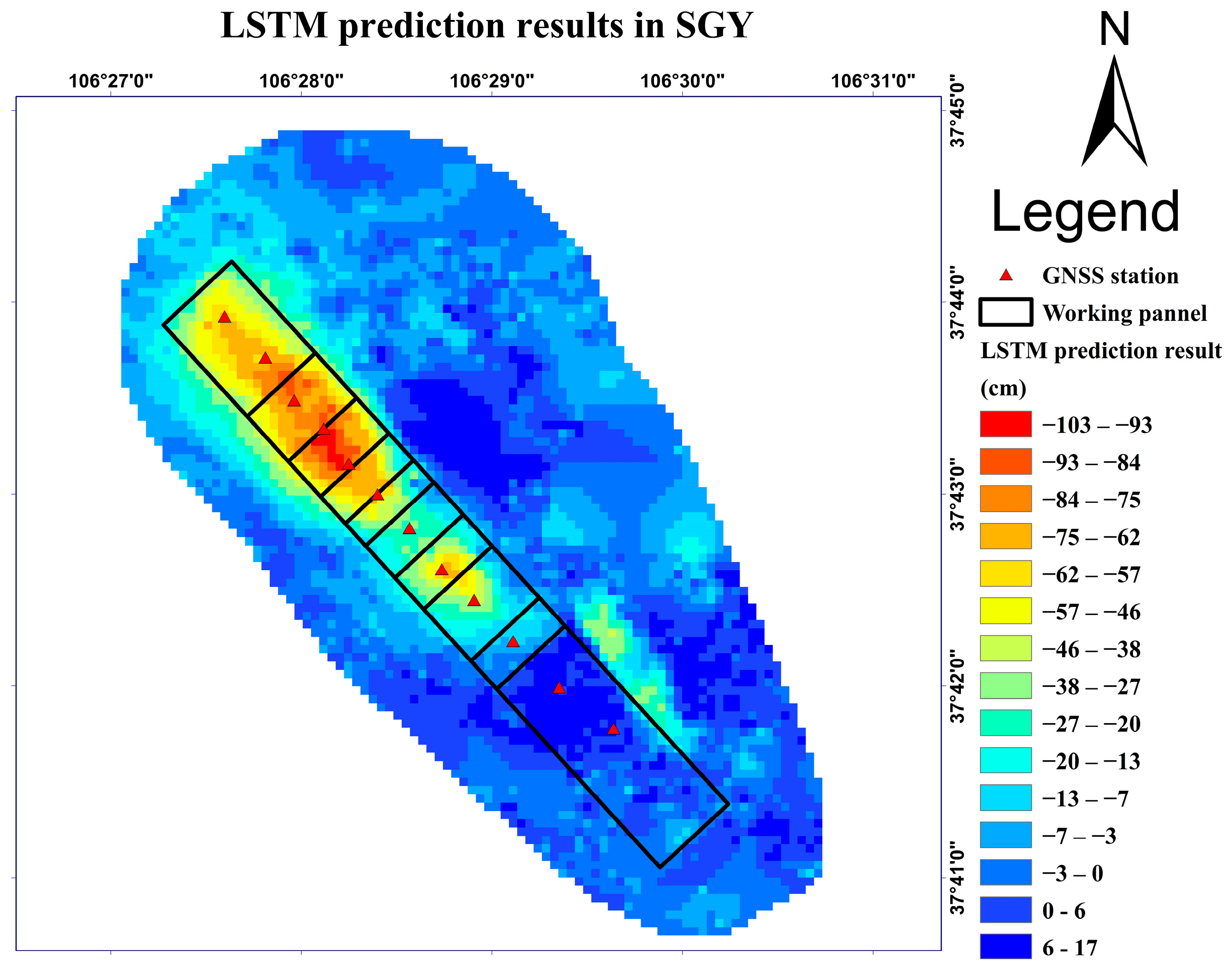
Figure 10 presents the settlement prediction results of the SGY mining area at the overall experimental scale. To obtain these results, the last 15 groups of deformation data from 20 May 2015 to 14 May 2016 were used as training samples to predict the deformation results of 7 June 2016. The predicted results were compared with the measured deformation results of InSAR, and the analysis showed a high degree of consistency between the predicted and real shape variables, indicating that the predicted settlement center area was clear and accurate. Moreover, the prediction errors of each monitoring point in the subsidence area were within 3 cm.
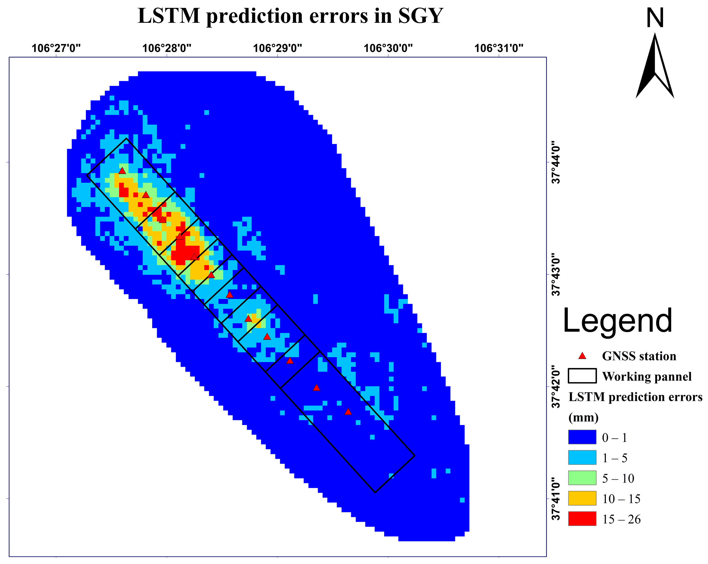
Figure 11 presents the prediction errors of LSTM. Out of 4795 observation points, the maximum difference (cumulative) shape variable had a prediction error of 2.6 cm, and the average prediction accuracy reached 93.6%. The calculation method of relevant indicators is given in Equations (9)–(12). Therefore, the model proposed in this paper has a small deviation when compared with the actual settlement amount, effectively reflecting the basic law of land surface settlement changing with time, and the predicted results are reliable.
4. Discussion
To assess the validity of the prediction model introduced in this study, GNSS observation stations situated on the surface of the mining area were selected for analysis. Real-time kinematic (RTK) technology utilizing the double-difference mode was employed across all stations, with a precision of up to 1 mm for horizontal displacement monitoring. As previously reported, the measurement error of elevation direction is approximately twice that of the horizontal displacement error [
52]. The monitoring values derived from the continuous time series deformation of the GNSS observation stations were extracted to verify the dependability of the prediction results obtained from the fusion of InSAR technology with LSTM. The table below exhibits the deformation values over time for each GNSS observation station based on their respective coordinates.
To demonstrate the superiority of the proposed prediction model, a comparison is made between the LSTM model and the traditional machine-learning model, using model establishment time and prediction error as evaluation metrics. Specifically, the SVR model is chosen as the representative of the traditional machine-learning model, which utilizes a nonlinear kernel function to map multidimensional inputs to higher dimensional feature space for regression analysis. In this study, the C penalty parameter and g kernel function parameter are optimized through the cross-verification method and grid search technique to identify the optimal parameter settings. Further details on the parameter searching process and experimental methodology can be found in [
53].
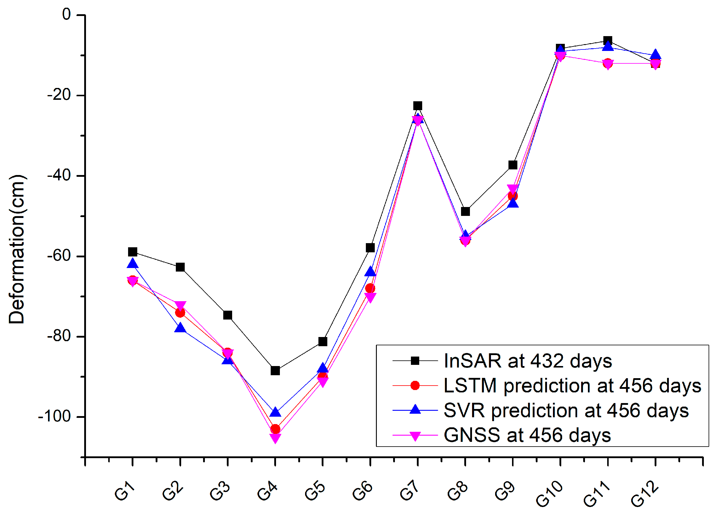
Table 3 presents the InSAR monitoring deformation cumulants of the SGY coal mine surface GNSS observation points over 432 consecutive days in the second column, while the third column displays the GNSS monitoring deformation cumulants over 456 consecutive days. Additionally, the fourth and fifth columns exhibit the cumulative shape variables predicted for 456 consecutive days by the LSTM algorithm and SVR algorithm, respectively.
Figure 12 corresponds to the data presented in
Table 3, showcasing the close proximity of the predicted values of the LSTM algorithm and the SVR algorithm to the GNSS monitoring results. Furthermore, the LSTM algorithm’s predicted values align with the GNSS monitoring values at multiple monitoring points, suggesting a high level of prediction accuracy. Thus, qualitatively, the results indicate the efficacy of the LSTM method in predicting cumulative shape variables.
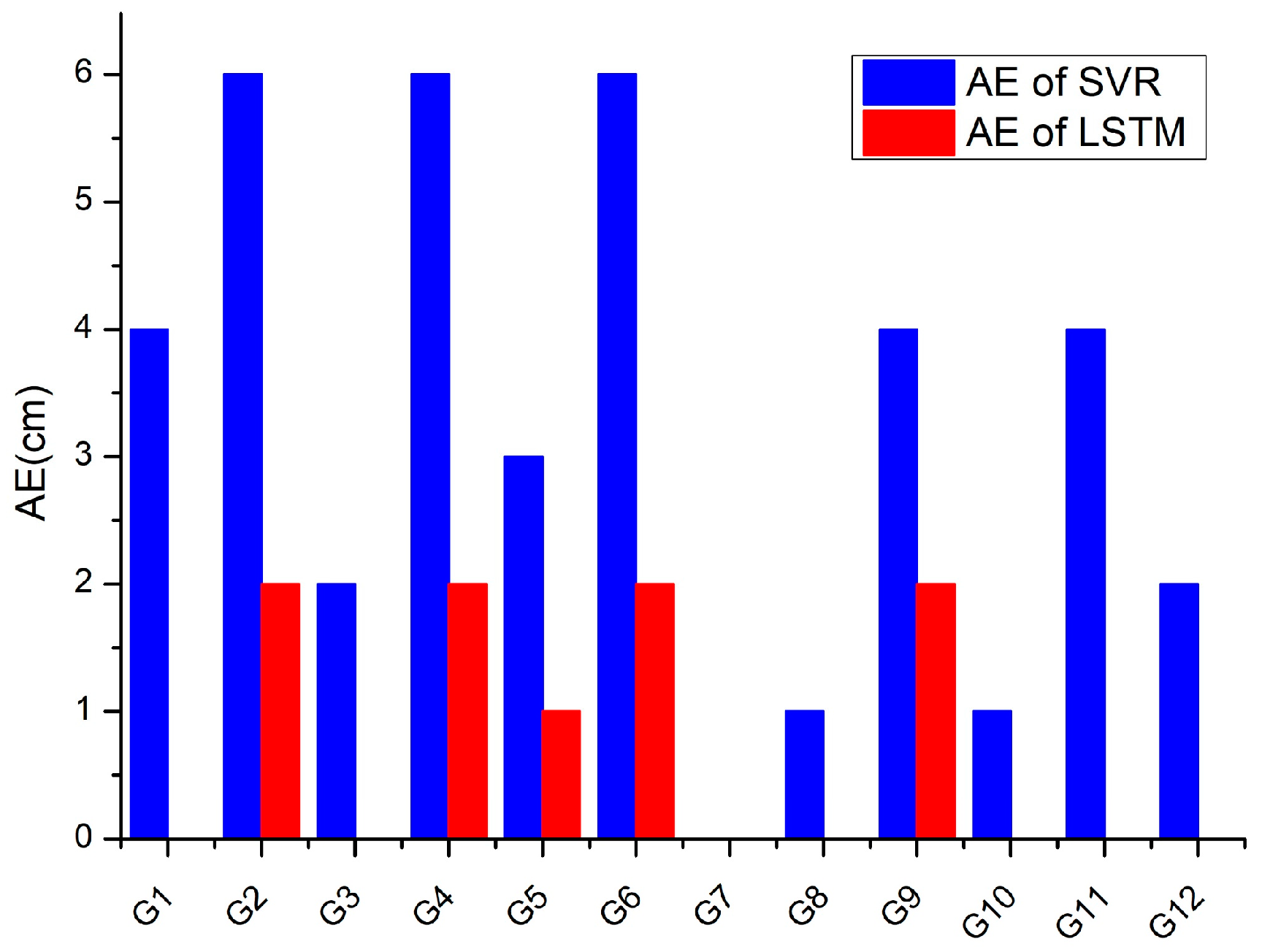
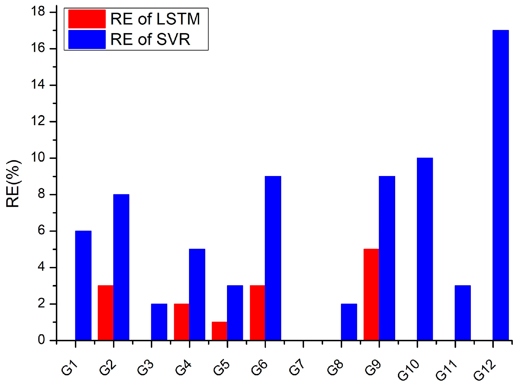
The bar charts displayed in
Figure 13 and
Figure 14 demonstrate the error distribution of prediction results for 12 GNSS monitoring points, revealing both the absolute and relative prediction errors of the LSTM and SVR prediction methods. These error metrics serve as quantitative indicators to assess the prediction accuracy of the two methods. The absolute and relative errors of the LSTM prediction at the 12 monitoring stations are smaller than those of the SVR prediction results. Specifically, the LSTM prediction method reports a zero error at G1, G3, G7, G8, G10, G11, and G12, whereas the SVR prediction method only has a zero error at the G7 observation station. The highest prediction error for both methods was observed at G2, G4, and G4 observation stations, with the LSTM method reporting an absolute error of 2 cm and the SVR method reporting an absolute error of 6 cm. This may be attributed to their central location within the subsidence basin, where mining activities were intensive over the 456-day inland. The deformation of these measuring points is influenced by multiple factors, such as geological structure, mining speed, and coal pillar, resulting in a more complex settlement pattern. The LSTM algorithm, with its superior learning ability, demonstrated a higher prediction accuracy compared to the SVR algorithm. Notably, the relative error between the predicted value and the truth value of the SVR method at the G12 station is at most 14%, with an absolute error of 2 cm. This is because G12 is situated at the edge of the subsidence basin with a relatively small subsidence value. However, the prediction accuracy of observation stations such as G1, G11, and G12 located in other subsidence basins is relatively high. These findings suggest that the LSTM method is better equipped to learn the intricate details of the settlement pattern.
Table 4 compares the prediction accuracy of the LSTM and SVR methods for the SGY coal mine. The table contains important error metrics such as the maximum absolute error, maximum relative error, average absolute error, and Wilmot consistency index, which provide a quantitative assessment of the accuracy of the prediction results.
The results in
Table 4 demonstrate that the LSTM model outperforms the SVR time series prediction method in terms of prediction accuracy. Specifically, the maximum prediction error of cumulative deposition using the LSTM model is less than 2 cm, while the maximum relative error and average relative error are lower compared to the SVR method. These findings indicate that the deep-learning-based prediction model proposed in this study is highly accurate and robust. The WIA and MAPE values for the LSTM model are 0.999 and 1.1%, respectively, and the Wilmot consistency index is close to 1, demonstrating the effectiveness of the prediction function established by Equation (13). The mining settlement prediction model based on InSAR monitoring data and LSTM is robust and outperforms the representative machine-learning model, SVR, in various evaluation indicators, including the Wilmot consistency index. Based on the above analysis, it is evident that the LSTM-based prediction method used for large-scale surface subsidence is highly accurate, efficient, and a better option to ensure production safety.
Comparative with the findings in references [
44,
45], it shows that the SBMHCT-InSAR technology improved from SBAS-InSAR is more suitable for deformation monitoring in mining areas. It can obtain the accurate deformation value of mining area surface, which is conducive to the training of the LSTM prediction model. The prediction results show that the prediction of mining area deformation by combining SBMHCT-InSAR technology and LSTM model is highly reliable and robust.


