Article

In-Situ GNSS-R and Radiometer Fusion Soil Moisture Retrieval Model Based on LSTM

1
College of Information Science and Engineering, Shandong Agricultural University, Tai’an 271018, China
2
School of Information Science and Engineering, University of Jinan, Jinan 250022, China
3
Shandong Provincial Key Laboratory of Network-Based Intelligent Computing, Jinan 250022, China
4
Beijing Institute of Spacecraft System Engineering, Beijing 100094, China
5
National Space Science Center, Chinese Academy of Sciences (NSSC/CAS), Beijing 100190, China
6
School of Electronic and Information Engineering, Beihang University, Beijing 100191, China
7
Environmental Remote Sensing Group (Climatology from Satellites), Earth Physics & Thermodynamics Department, Faculty of Physics, University of Valencia, 46100 Valencia, Spain
*
Author to whom correspondence should be addressed.
Remote Sens. 2023, 15(10), 2693; https://doi.org/10.3390/rs15102693
Submission received: 11 April 2023 / Revised: 11 May 2023 / Accepted: 20 May 2023 / Published: 22 May 2023

Abstract

:
Global navigation satellite system reflectometry (GNSS-R) is a remote sensing technology of soil moisture measurement using signals of opportunity from GNSS, which has the advantages of low cost, all-weather detection, and multi-platform application. An in situ GNSS-R and radiometer fusion soil moisture retrieval model based on LSTM (long–short term memory) is proposed to improve accuracy and robustness as to the impacts of vegetation cover and soil surface roughness. The Oceanpal GNSS-R data obtained from the experimental campaign at the Valencia Anchor Station are used as the main input data, and the TB (brightness temperature) and TR (soil roughness and vegetation integrated attenuation coefficient) outputs of the ELBARA-II radiometer are used as auxiliary input data, while field measurements with a Delta-T ML2x ThetaProbe soil moisture sensor were used for reference and validation. The results show that the LSTM model can be used to retrieve soil moisture, and that it performs better in the data fusion scenario with GNSS-R and radiometer. The STD of the multi-satellite fusion model is 0.013. Among the single-satellite models, PRN13, 20, and 32 gave the best retrieval results with STD = 0.011, 0.012, and 0.007, respectively.

Graphical Abstract

1. Introduction

Soil moisture is an essential parameter in hydrology, agriculture, and meteorology. In agriculture, soil moisture is an integral part of crop moisture prediction [1] and an essential basis for organising irrigation and crop yield estimation. In relation to weather prediction, numerical simulation weather prediction models show that the introduction of boundary conditions such as surface soil moisture, vegetation indices, and ground temperature data can significantly improve the accuracy of the prediction. Soil moisture measurements on a global or regional scale have therefore great social and economic advantages. From this point of view, the traditional techniques for measuring in situ soil water content become impractical when dense spatial and temporal resolutions are required. Compared to the traditional contact-type soil moisture sensing technologies such as time domain reflectometry (TDR) and frequency domain reflectometry (FDR), microwave remote sensing technology can better achieve large-scale, non-contact soil moisture detection [2]. Among these, passive microwave remote sensing uses microwave emissivity to retrieve soil moisture [3]. Although it is sensitive to soil moisture and has high temporal resolution, its spatial resolution is low and cannot yet meet the application’s needs. In contrast, synthetic aperture radar (SAR) uses a self-contained source of microwave radiation to illuminate the surface and measures the amount of radiation returned to the sensor. This allows SAR to monitor surface soil moisture at a spatial resolution of meters to tens of meters under almost all weather conditions [4,5]. Nonetheless, it still has inherent complexity related to the radar backscattered signal and to the inverse problem of backscattering models [6]. During the last few decades, an emerging and challenging technology based on signals of opportunity, composed of receiving devices that take advantage of existing signals from other systems, is being exploited for specific Earth observation applications such as the determination of the geoid, wind speed at the sea’s surface, and surface soil moisture and vegetation water content [7]. Among these, the technology that employs global navigation satellite systems (GNSS) is called GNSS reflectometry (GNSS-R). According to recent studies, GNSS-R has proven its ability to retrieve soil moisture and vegetation water content from the ground, while airborne, and in spaceborne configurations [8].
Kavak et al. [9] first investigated the sensitivity of the GNSS signal reflected from the ground surface to the latter’s moisture content, and Zavorotny and Voronovich [10,11] provided the first theoretical model of GNSS signal-scattering. In 2002, NASA and the University of Colorado added a GPS-R receiver to the airborne soil moisture measurement experiment SMEX02 (Soil Moisture Experiment 2002), which showed that the intensity of the reflected signals was related to soil moisture [12]. ESA and Starlab conducted, in 2009 and 2011, respectively, the LEiMON (Land Monitoring with Navigation Signals) and GRASS (GNSS Reflectometry Analysis for Biomass) GNSS-R ground and airborne tests to study the effects of soil moisture, surface roughness and vegetation parameters on GPS reflection signals under different polarisation conditions [13]. Egido et al. conducted flight experiments on a low-altitude airborne platform, the results of which showed that, in the case of moderate roughness, the polarised reflectivity ratio represented the best-observed value of soil moisture, with a correlation coefficient of 0.93 [14]. Following the successful launch of the NASA CYGNSS (Cyclone Global Navigation Satellite System), soil moisture estimation was tested by adopting different methods to process the derived data, and global soil moisture estimates were obtained with a global spatial resolution of 36 × 36 km² and RMSE of 0.07 cm³/cm³ [15].
Normally, the ground’s surface is relatively rough at L-band microwaves, so the influence of surface roughness must be taken into account when retrieving soil moisture using GNSS-R. The L-MEB (L-band microwave emission of the biosphere) model for microwave radiometry [16] can retrieve brightness temperature TB, and the TR indices (representing the combination of vegetation optical thickness and soil roughness) provide information sufficient to remove the impacts of vegetation cover and ground surface roughness. On this line, Fernandez-Moran et al. proposed a simplified retrieval method (SRP) to accurately account for surface roughness and vegetation optical depth effects in soil moisture retrievals. The τ N A D (vegetation optical depth at nadir) and H R (L-MEB model roughness parameters) can be grouped and retrieved as a single parameter called TR [17]. Cong et al. compared GNSS-R and ELBARA-II radiometer data, a high correlation was found between the LHCP reflectivity measured by GNSS-R and the horizontal/vertical reflectivity from the radiometer. An artificial neural network was used for GNSS-R soil moisture retrieval, and the RMSE was 0.014 m³/m³ [18]. However, the artificial neural network cannot take advantage of a soil moisture time series. In time series, data from each point in time will be affected by the previous points. Recurrent neural networks (RNN) appeared in the 1980s and 1990s. Through the connection between nodes, it receives the output information froms the current time and the output information of the previous time at the same time and then form a network structure with circulation to facilitate learning the nonlinear characteristics of the timing sequence efficiently [19,20].
In this paper, a GNSS-R soil moisture retrieval model based on a LSTM (long–short term memory) neural network is proposed. TR and TB of a ground-based radiometer are introduced in the proposed model to eliminate the influences of soil roughness and vegetation effects, as indicated above. Finally, the proposed model is verified by the joint observation campaign of the passive ground-based microwave remote sensing ELBARA-II and of the dual-antenna GNSS-R Oceanpal at the Valencia Anchor Station, a remote sensing validation site in Spain [18].

2. Methods

2.1. Traditional GNSS-R Retrieval Model

With the change of soil moisture in the surface layer, its dielectric constant also changes, thus affecting the reflected signal intensity, which is the principle by which GNSS-R technology can detect soil moisture. As shown in Figure 1, traditional GNSS-R is a bi-static radar configuration, one which uses the GNSS satellite and receiver as radar transmitter and receiver, respectively. The direct GNSS signal is right-hand circularly polarised (RHCP), but when reflected by the ground’s surface, the reflected signal will contain both left-hand circularly polarised (LHCP) and right-hand circularly polarised (RHCP) components. As the satellite’s elevation angle increases, the right-handed component of the reflected signal gradually decreases, and the left-handed component gradually becomes the dominant component.
The reflection coefficient of a left-hand reflected signal can be expressed by Equation (1):
Γ rl = R r l ( ε , θ ) 2 = ( ε 1 ) 2 cos 2 θ ( ε sin 2 θ ) ( ε cos θ + ε sin 2 θ ) 2 ( cos θ + ε sin 2 θ ) 2
Γ rr = R r r ( ε , θ ) 2 = ( ε 1 ) 2 sin 4 θ ( ε sin θ + ε sin 2 θ ) 2 ( cos θ + ε sin 2 θ ) 2
where ε is the relative permittivity of the reflecting surface, and θ is the elevation angle of the GNSS satellite [21].
The soil dielectric constant is mainly determined by water content so that soil moisture can be retrieved through it. Therefore, the basic idea of GNSS-R soil moisture retrieval model is to establish the relationship among reflection coefficient, permittivity and soil moisture (Figure 2). Although the theoretical model of the soil dielectric constant can be described in detail, the relationship between soil dielectric constant and water content could be given either by soil dielectric model such as Wang model [22], the Topp model [23], the Hallikainen model [24], or the Dobson model [25] and so on.
With the exception of Wang’s model, the model structure and the information required are too complex to use, and therefore Wang’s model was selected for soil moisture retrieval in this work. The model can be expressed by Equation (3):
ε = 3.1 + 17.36 m v + 63.12 m v 2 + j ( 0.031 + 4.65 m v + 20.42 m v 2 )
where ε is the permittivity of the soil and m v is volumetric water content of the soil. By introducing the soil dielectric constant obtained by Equation (1) into Equation (3), the results of GNSS-R soil moisture retrieval can be expressed by Equation (4):
m v = 17.36 + 17.36 2 252.48 3.1 ε 126.24

2.2. ELBARA-II

This traditional GNSS-R retrieval method does not take into account the influence of surface roughness and vegetation, so the retrieval accuracy can be optimised. Between 2014 and 2016, a joint observation experiment was carried out using the ground-based radiometer ELBARA-II and the Oceanpal dual-antenna GNSS-R receiver at the Valencia Anchor Station [18]. This section presents a method to extract surface roughness and vegetation influencing factors from ELBARA-II data and feed them into a soil moisture retrieval model based on a non-linear auto-regressive dynamic neural network to improve retrieval accuracy.
The ground-based microwave radiometer (ELBARA-II, L-band) is a Dicke-type L-band microwave radiometer ( f = 1.41 GHz, λ = 21 cm) developed by the Swiss Federal Research Institute for Forest, Snow, and Landscape (WSL) together with GAMMA remote sensing from the European Space Agency (ESA) [26]. It was designed mainly for SMOS validation and to improve its L-band soil moisture retrieval algorithm, thus providing significant ground reference data for the L-band passive microwave radiation transmission model. ELBARA-II adopts the optimal dual polarisation (P = horizontal polarisation-H, = vertical polarisation-V) cone antenna design (diameter 1.4 m, antenna length 2.7 m, −3 dB bandwidth of 11 MHz), as shown in Figure 3. It has two 11 MHz synchronous channels centred at 1.4075 GHz and 1.4195 GHz, respectively, which allow narrow-band RFI to be detected within the protected L-band. The absolute error of ELBARA-II brightness temperature observation is less than 1.0 K, and it can sensitively respond to microwave brightness temperature changes greater than 0.1 K [26].
The polarisation brightness temperature T B p observed by the L-band ELBARA-II radiometer at different incident angles α, and the influence of the surface characteristics on it, can be described by the L-MEB microwave radiation model, as in Equation (5) [16]:
T B p ( θ ) = T G C [ 1 r G P ( θ ) exp ( 2 τ N A D cos 2 ( θ ) + t t p sin 2 ( θ ) cos ( θ ) H R cos N R P ( θ ) ) ]
where T B p is the brightness temperature observed by the microwave radiometer, T G C is the composite soil-vegetation surface temperature, r G P is the Fresnel reflectance of the soil surface, t N A D is the optical thickness, H R accounts for the decrease of specular reflectivity due to soil roughness effects, and θ is the observation angle. The subscript p indicates the polarisation mode; t t p is a parameter used to quantify the dependence of t N A D on the incidence angle θ and N R P governs the changes in the angular dependence of reflectivity, thus quantifying the dependence of H R on the incidence angle θ [17].
Under low-frequency L-band conditions, if the dependence of roughness on the incident angle under different polarisation modes can be assumed as N R V = N R H = 1 , then the influence of vegetation can be regarded as isotropic and Equation (5) can be simplified as Equation (6):
T B p ( θ ) = T G C [ 1 r G P ( θ ) exp ( 2 T R / cos ( θ ) ]
T R = τ N A D + H R / 2
In that case, the effects of vegetation (via the t N A D parameter) and roughness (via the H R parameter) can be combined into the single parameter TR, defined in Equations (5) and (6) [17]. The model uses the two-parameter retrieval method to find the optimal solution of TR based on the iterative form of the least squares method. The parameters are then fed into the GNSS-R soil moisture retrieval model, based on the LSTM neural network.

2.3. LSTM Neural Networks

LSTM is an RNN that underlies sequential learning applications [27]. As a type of RNN, LSTM uses sequential information by updating states based on both inputs from the current time step ( x t ) and network states from previous time steps. However, the architectural difference from RNNs is that LSTM has ‘memory states’ units and ‘gates’ that are trained to decide when they can forget some information, when and what to output, and which inputs to use. These gates are also responsible for learning and memorizing the data characteristics of soil moisture. The common structure of the LSTM neuron cell is demonstrated in Figure 4.
The following equations are included in the LSTM neuron:
The σ function:
δ ( x ) = 1 1 + e x
Forget Gate:
f t = δ ( W f [ h t 1 , x t ] + b f )
Input Gate:
i t = δ ( W i [ h t 1 , x t ] + b i )
C t = e ( W c [ h t 1 , x t ] + b o ) e ( W c [ h t 1 , x t ] + b o ) e ( W c [ h t 1 , x t ] + b o ) + e ( W c [ h t 1 , x t ] + b o )
Output Gate:
o t = δ ( W o [ h t 1 , x t ] + b o )
Long Memory:
C t = f t C t 1 + i t C t
Short Memory:
h i = o t e C t e C t e C t + e C t
where C is the cell state, W is the corresponding weight coefficient matrix, and b is the corresponding bias term. Firstly, the input x t at time t and the hidden state h t 1 at time t 1 discard distant information through the forgetting gate to obtain an updated value f t . Next, x t and h t 1 pass through the input gate to obtain the data i t to be updated and the new candidate vector C t . Finally, x t and h t 1 pass through the output gate to obtain the output result o t of the neuron. The cell state C t at time t is obtained by summing the inner product of f t and C t 1 and the inner product of i t and C t , and the new cell hidden state h t is obtained by summing the value of the hyperbolic tangent of the cell state C t at time t and o t . By repeating the above process, the LSTM neural network composed of multiple neurons can be trained [28].
Before building the prediction model, we have to set several hyperparameters of the LSTM prediction network structure, including the number of LSTM layers, the number of nodes in each LSTM layer, the number of fully connected layers (FC), and the number of nodes in each level of the FC layer, as well as the epoch and the learning rate. The LSTM network of this work consisted of five layers, an input layer, an LSTM layer, a drop layer, a fully connected layer, and an output layer. The number of nodes, the learning rate, and the epoch use the Bayesian optimisation method to find the optimal value (Figure 5).

2.4. Bayesian Optimisation

Parameter optimisation is an indispensable step in building neural network models. The common problem of finding the extremum of a function can be solved by gradient-based optimisation [29]. However, traditional grid search requires training on each parameter combination, which is highly time-consuming. The Bayesian optimisation algorithm is a black-box optimisation algorithm that does not need to know the expression of the objective function. It uses a straightforward framework to find the optimal global solution, and the optimisation process saves time, so it is very suitable for adjusting the parameters of the LSTM [30].
In the Bayesian optimisation process, the loss function of the parameter-fitting model is a Gaussian process, and the parameters are updated to obtain the posterior probability of this function. The process of Bayesian optimisation is described as follows:
The Bayesian optimisation objective is defined as:
x min = arg min x X f ( x )
where x min is the final optimised hyperparameter and f ( x ) is the objective function to be optimised.
Assuming that the hyperparameters to be optimised are X = { x 1 , x 2 , , x i } , the data set obtained by Bayesian optimisation iteration is
D t = x 1 , f ( x 1 ) , x 2 , f ( x 2 ) , , x t , f ( x t )
The Gaussian process assumes that the observation points follow a Gaussian distribution with the following expression:
f ( x ) ~ G P μ ( x 1 : t ) , n ( X 1 : t , X 1 : t )
where n ( X 1 : t , X 1 : t ) is the covariance matrix:
n ( X 1 : t , X 1 : t ) = k ( x 1 , x 1 ) k ( x 1 , x t ) k ( x t , x 1 ) k ( x t , x t )
According to Bayes’ theorem:
P f ( x t + 1 ) f ( x 1 : t ) P f ( x 1 : t ) f ( x t + 1 ) P f ( x t + 1 )
By iteratively updating x min = x i + 1 , the optimal hyperparameters are finally obtained.

2.5. Uncertainty Analysis

The predicted models’ uncertainty must be quantified in order to confirm the validity of the model [31]. All soil samples were randomly divided between training (70%) and validation (30%) for each iteration of the uncertainty analysis in order to train 50 distinct LSTM models. Due to the implicit time information in the data, they cannot be randomly divided. Therefore, we carried out the uncertainty analysis by adjusting the proportion of training and testing sets (the first 80% of the data used for training, and the last 20% used for test or the first 60% of the data used for training, and the remaining 40% used for test).

3. Results

3.1. Experiment Campaign

The Valencia Anchor Station validation site is located on the Utiel–Requena plateau, 80 km northwest of Valencia city, Spain, and the SOMOSTA (Soil Moisture Monitoring Station) experiment took place at the Valencia Anchor Station MELBEX (Mediterranean L-band characterization experiment) site within the El Renegado vineyard area, with coordinates (39°31′17.98″N, 1°17′29.29″W) and an altitude of 800 m. During this experimental campaign, the ESA GNSS-R Oceanpal antenna was installed on the same tower as the ESA ELBARA-II passive microwave radiometer, the Ocenapal at 11 m height from the ground, while ELBARA-II had previously been installed at the top of the tower at a height of 15 m, and both measuring instruments had a similar field of view. ELBARA-II automatically adjusts the incident angle every half hour to measure brightness temperature (TB) from several consecutive angles, ranging from 30° to 70° at 5° intervals. The incident angle range of the observations used in the soil moisture inversion model was 30~55°. Oceanpal has an upward right-hand circularly polarised antenna that receives the direct signal, and a downward left-hand/right-hand circularly polarised antenna receiving the reflected signal from the ground. Both antennas were assumed to have the same antenna pattern thanks to a calibration tool that minimised possible differences between the two channels (Figure 6). The angle between the direct antenna and the reflection antenna was 20°, and they were installed in mirror symmetry relative to the horizontal direction to eliminate the impact of antenna gain, as shown in Figure 6 and Figure 7. On the one hand, this avoids the influence of the observation tower on the signal and, on the other, it facilitates a larger observation area.
Two ML2x ThetaProbe soil moisture sensors were installed under the observation tower to collect in situ soil moisture data to verify retrieval precision. The distance between the probes was 1.5 m. The sensor’s accuracy was ±1%, and the sampling interval was 2 min. As shown in Figure 8, both sensors were 5 cm deep under the soil’s surface. One sensor was placed under a vine stock and the other between two rows of vines. In addition, the observation tower also had a Davis Vantage Pro 2 weather station, which is used to measure precipitation, temperature, wind and humidity.
Radiometer-related data such as brightness temperature (TB), soil roughness and vegetation attenuation index TR where obtained by using the L-MEB radiative transfer model (Equations (5) and (6)). GNSS-R data is processed according to Equation (4). Experimental data from ELBARA-Oceanpal are then used for validation and optimisation. Figure 9 shows the variation of Rrl (left-hand circularly polarised reflectivity) with elevation angle, and the scattered colour indicates the value of the azimuth angle. Rrl does not depend on the azimuth angle, and reflectivity is distributed in the range of 0.1–0.4 with the same elevation angle. Therefore, in this experiment, in the presence of vegetation cover, the influence of azimuth can be ignored, and the surface can be considered an isotropic reflecting surface.
The GNSS-R Oceanpal observations lasted from October 2014 to May 2016. During the experiment, there were several interruptions of the observations for various reasons (in summer, sometimes the temperature in the hut containing the equipment could become too high, interrupting the computers and the power supply, although in the end a magneto-thermal control system was installed and even a shunt to ground to avoid lightning damage in times of heavy rain). The applicable soil moisture range of the Wang model mentioned earlier is 0–0.5 [22,32]. It follows from Equation (3) that the theoretical reflectivity range of Wang’s model is 0–0.4, so data with reflectivity higher than 0.4 are removed. Since precipitation causes a large amount of water on the surface, which causes an abnormal increase in reflectivity and affects the reception of the reflected signals, data from the day of precipitation and the following day are also removed, thus completing the data quality screening. Finally, 180 days of complete observational data are available, including GNSS reflectivity, ELBARA-II radiometer brightness temperature observations, and ground-based soil moisture measurement observations. The data processing flow is shown in Figure 10.

3.2. Results Derived from the Analytical Model

Figure 11 shows the retrieval results for the Wang model and for ELBARA-Ⅱ radiometer. The retrieval accuracy of the Wang model is low. Compared to the Wang model, the effect of ELBARA-Ⅱ has been dramatically improved. In this figure it can be seen that, compared to the in situ probes, there was a systematic error (0.101 m³/m³) in the ELBARA-Ⅱ retrieval result, so we corrected the ELBARA-Ⅱ retrieval results as to that amount. The correlation coefficient reaches 0.78, and the RMSE decreases to 0.024 (Table 1).
It is assumed that soil moisture does not vary significantly from one hour to the next, which is fully valid in the absence of precipitation, since precipitation sharply increases soil moisture in a short period of time. Thus, we took mean hourly values of the Wang model and of the ELBARA-II radiometer output results, respectively (Figure 12). As shown in Table 2, the correlation coefficient of the Wang model inversion results increases to 0.26, and the RMSE decreases to 0.087, whereas the correlation coefficient of ELBARA-Ⅱ increased to 0.83, and the RMSE decreased to 0.098 and to 0.024 after the correction mentioned above (Table 2). However, due to its low temporal resolution, the soil moisture value was output at 6 a.m. and 6 p.m., and it is necessary to adjust it in the comparison time scale.

3.3. Results Derived from LSTM Model Retrieval

3.3.1. Results Derived from Multi-Satellite LSTM Model Retrieval

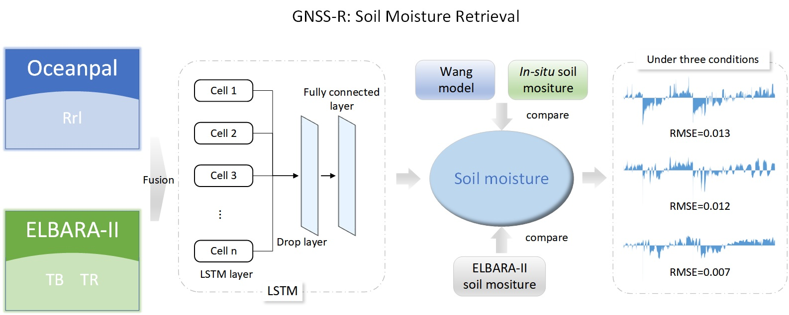
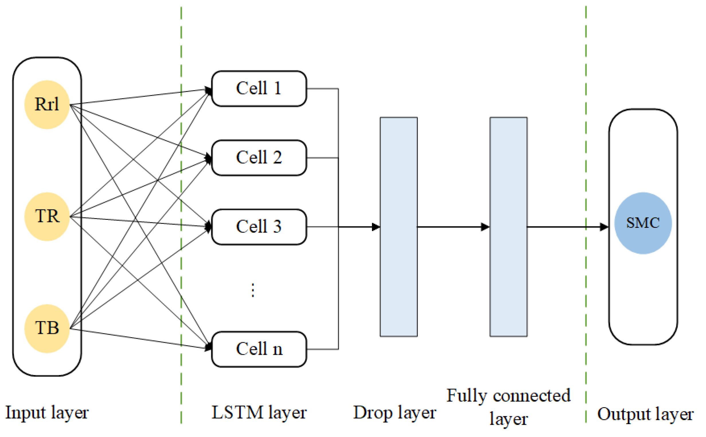
Using Rrl as input data, combined with TB and TR as auxiliary data, the optimal parameters of the LSTM network were found by a Bayesian optimisation algorithm for 100 iterations, and the LSTM soil moisture retrieval model was established. The field measurement value of the ThetaProbe soil moisture sensor was used as the target setting for training. The first 70% of the experimental data (1 October 2014–24 March 2016) was used for training, and the last 30% (25 March 2016–31 March 2016) was used as the test set for model prediction and evaluation.
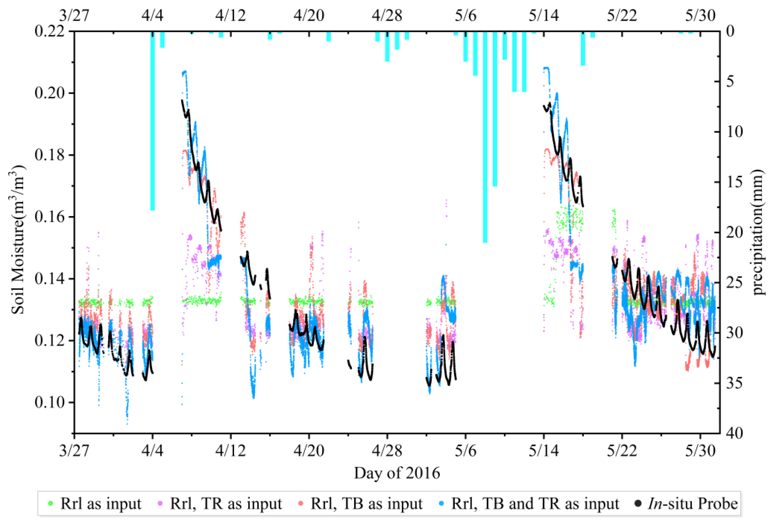
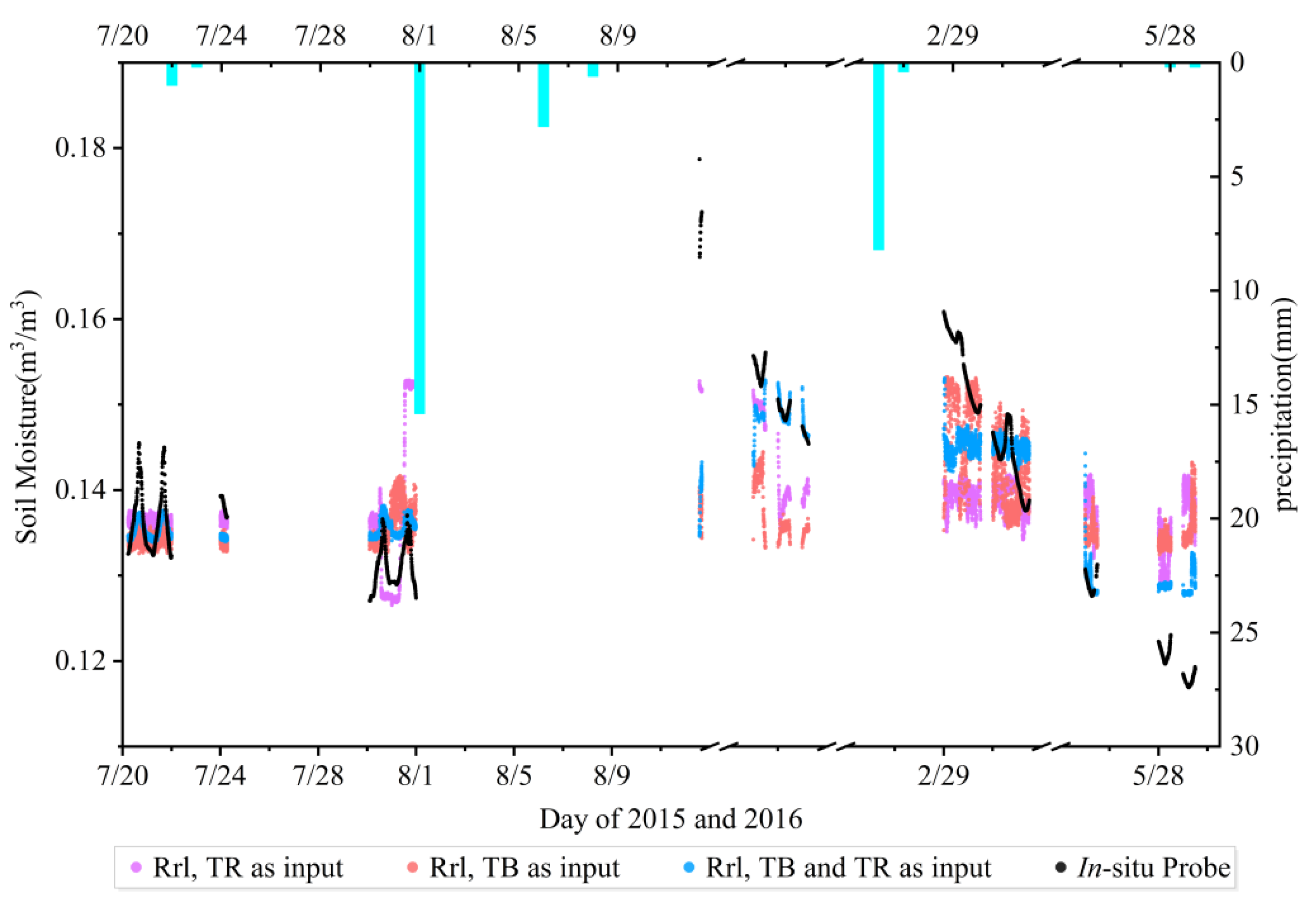
The results are shown in Figure 13. Compared to the black dots in situ, the blue and red dots in the figure match better, the purple dots less well, and the green dots worse. When Rrl as such (green) is used as input data for the prediction, the correlation coefficient is only 0.50, and the RMSE is 0.019. When only Rrl is used as input data, the retrieved soil moisture obtained fluctuates only around 0.13 m³/m³, which does not reflect the real soil moisture change. This is because the reflectivity data are mixed with a lot of noise. The model cannot extract features well in the case of a single input variable, which causes the soil moisture recovery to show almost a straight horizontal line. The accuracy is poor, so the subsequent multi-satellite soil moisture retrieval no longer uses only 
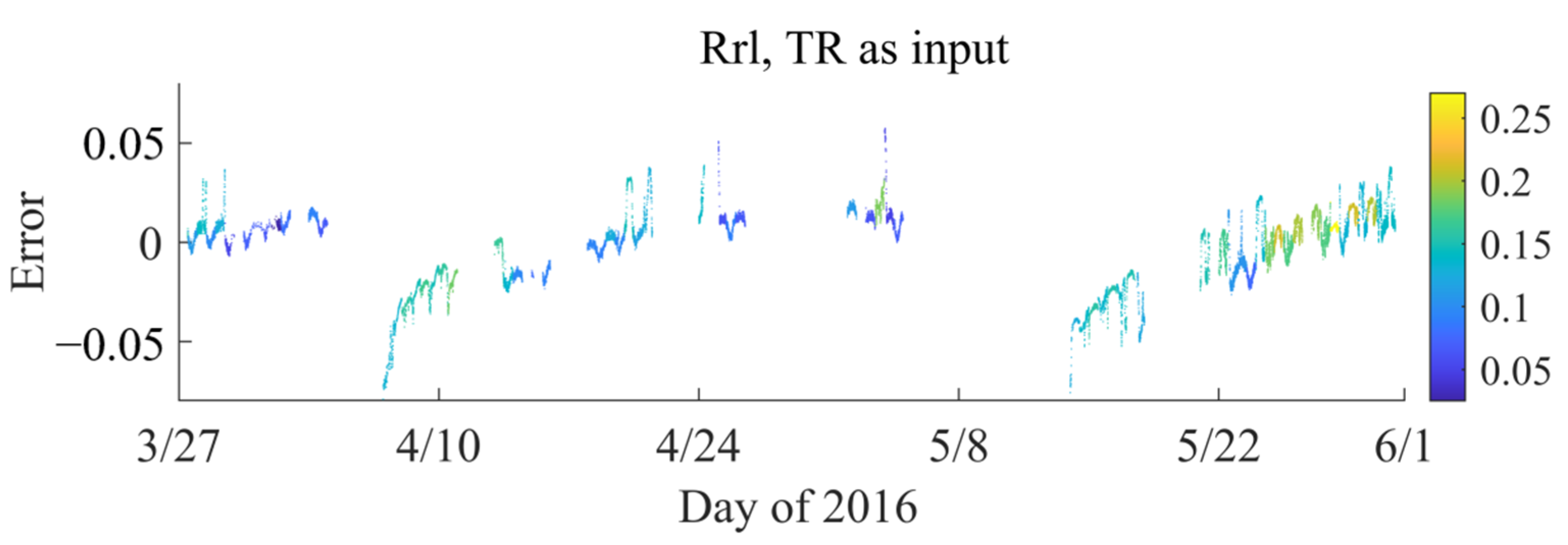
Rrl as input data. When Rrl is used as input data for prediction together with TR, the correlation coefficient improves to 0.58, and the RMSE is reduced to 0.018 m3/m3. When Rrl is used as input data for prediction together with TB, the correlation coefficient improves to 0.81, and the RMSE decreases to 0.013. Finally, when Rrl, TR, and TB are used together as input data for prediction, the correlation coefficient increases to 0.83, and the RMSE decreases to 0.013 (Table 3).
Subsequently, we performed an uncertainty analysis of the model. According to Table 4, the performance of the models under different data allocation methods is good, thus implying that the model has low variability and low uncertainty.
For comparison, we used the multilayer perceptron with backpropagation learning algorithm (MLP-BP) and support vector machine (SVM) to retrieve soil moisture [33,34]. Table 5 showed that the results of MLP-BP and SVM were not as good as those of LSTM. Therefore, in following studies, we only used the LSTM model to retrieve soil moisture.
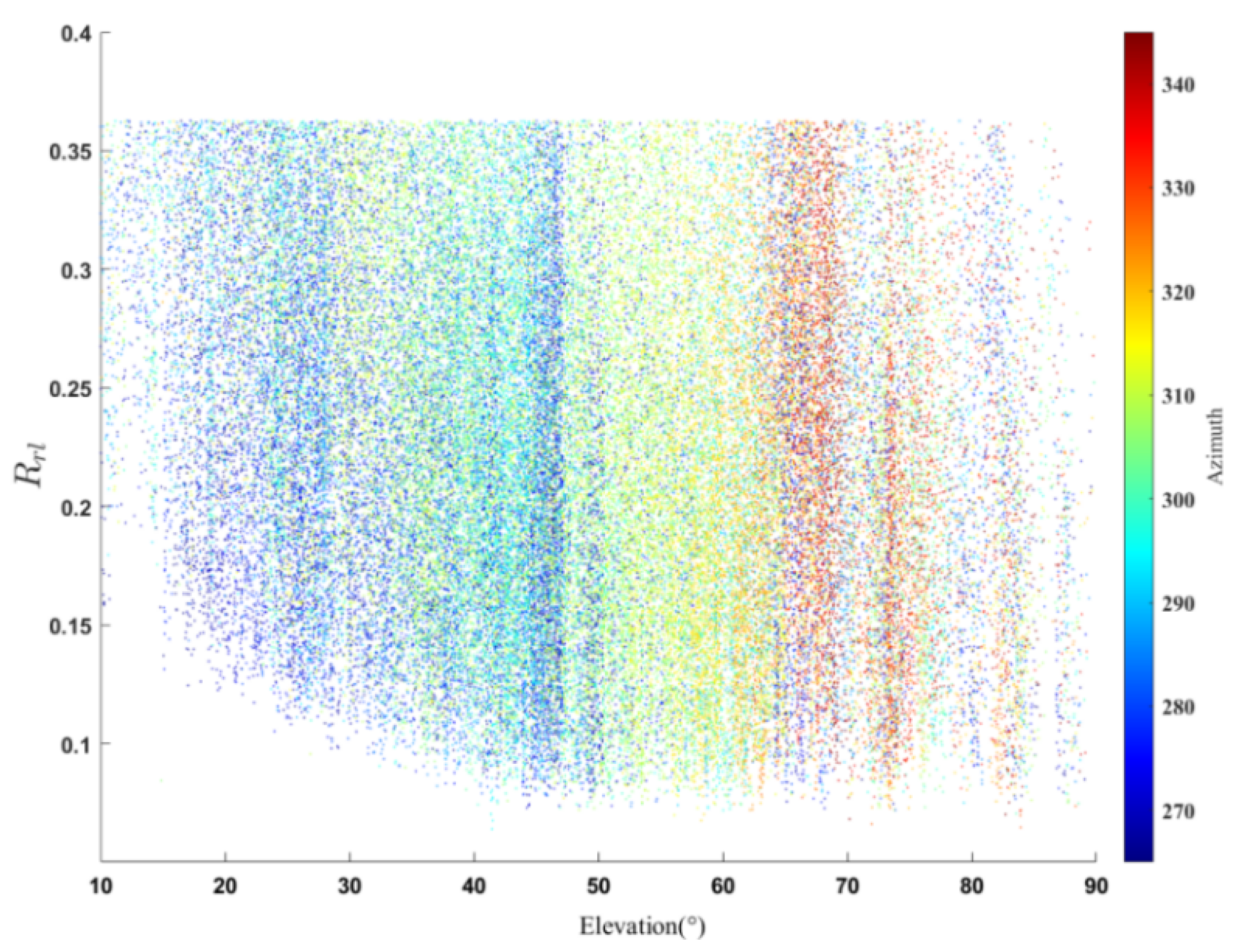
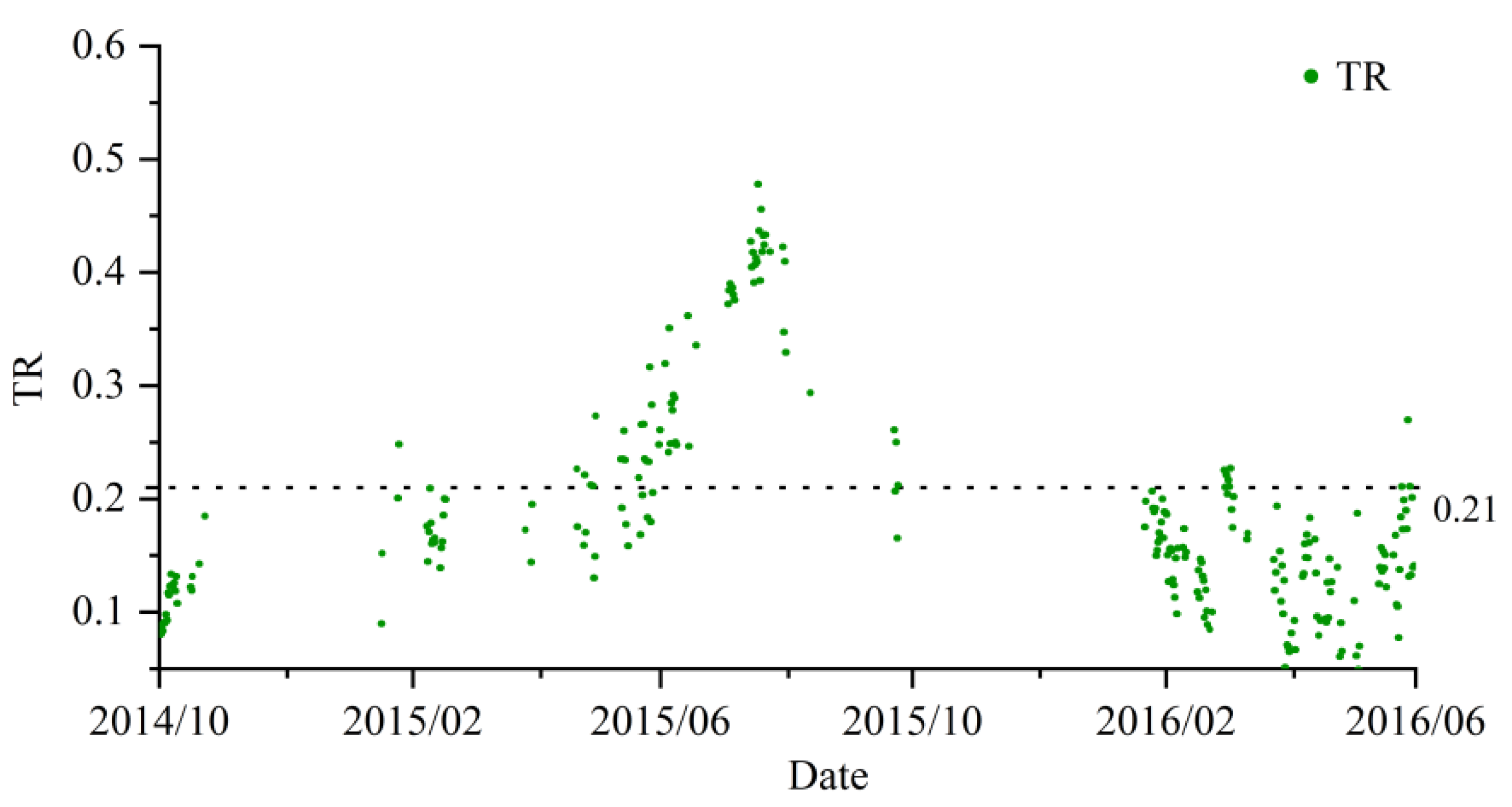
Because soil surface roughness, vegetation scattering, and other factors affect the accuracy of model retrieval, more carefully distinguishing model performance under different roughness conditions still improves accuracy. This section analyses the retrieval accuracy of two models with different roughness conditions. Since the LSTM model is applied to continuous time series, the roughness threshold is set to 0.21, considering that data above 0.21 corresponds to high roughness, and data below 0.21 corresponds to low roughness (Figure 14). In this section, the model is trained and prepared for prediction under two different roughness conditions.
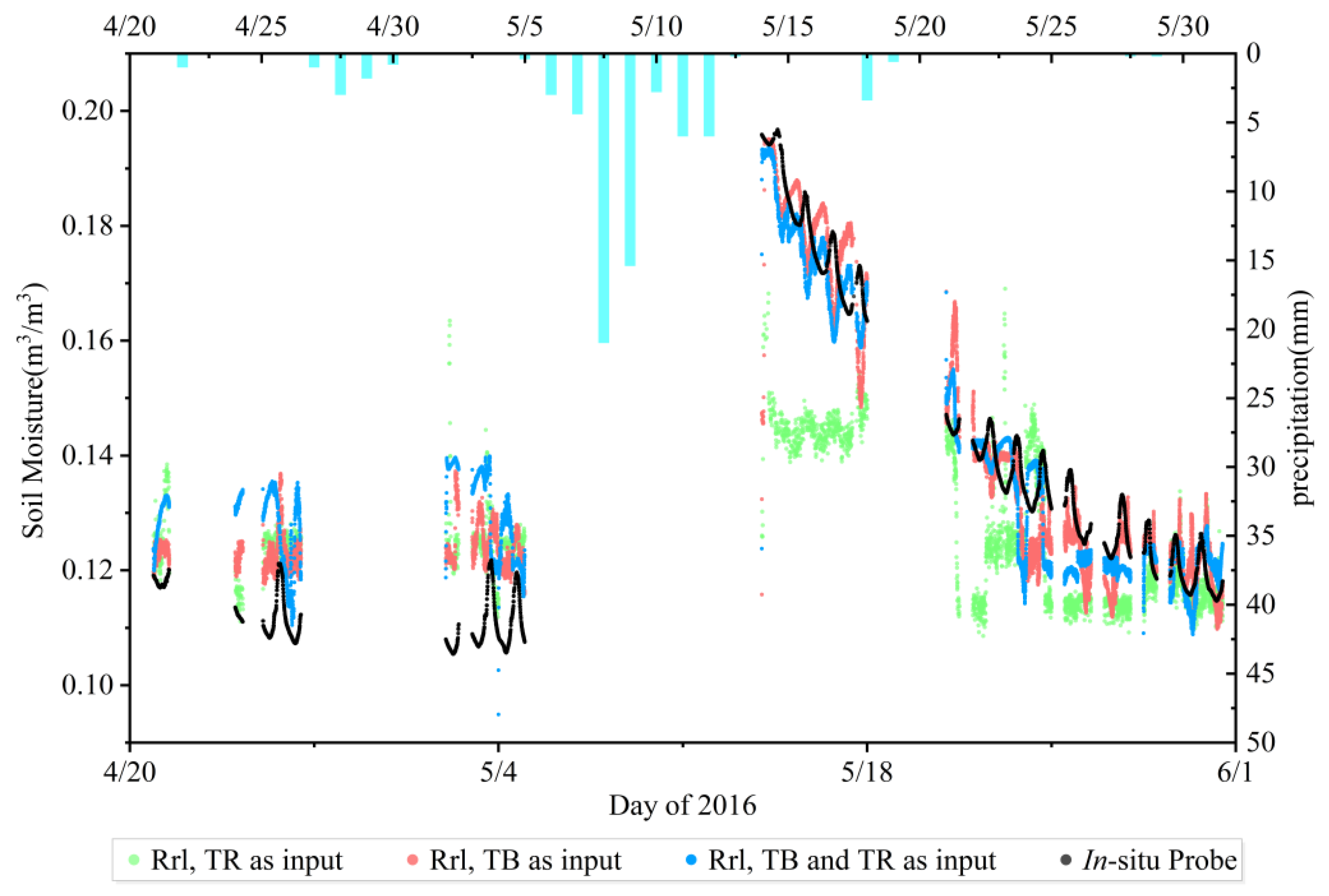
According to the threshold, in this first analysis, experimental data with high roughness are discarded, amounting to a total of 37,783 moments. Similarly, Rrl, TB, and TR are selected as input data, and the training set and the test set are divided according to the standard ratio of 70% and 30%, respectively, where the training set has 26,448 moments, and the test set has 11,335 moments for training and prediction. In Figure 15, the red dots and black dots match better. When Rrl is used as input for prediction together with TR, the correlation coefficient is 0.67, and the RMSE is 0.017. When Rrl is used as input for prediction with TB, the correlation coefficient improves to 0.90, and the RMSE decreases to 0.009. When Rrl is used as input for prediction together with TR and TB, the correlation coefficient is 0.85, and the RMSE is 0.012 (Table 6).
Similarly, in the second analysis, experimental data with low roughness are discarded, amounting to a total of 24,509 moments, including 17,156 moments in the training set and 7353 moments in the test set, for training and prediction. Figure 16 shows the prediction effect of the model in high roughness, where the blue dots and black dots match better. When Rrl is used as input for prediction with TR, the correlation coefficient is only 0.36, and the RMSE is 0.010. When Rrl is used as input data for prediction with TB, the correlation coefficient improves to 0.53, and the RMSE is reduced to 0.009. When Rrl is used as input data for prediction together with TR and TB, the correlation coefficient is 0.83, and the RMSE is 0.007 (Table 7).

3.3.2. Results Derived from Single-Satellite LSTM Model Retrieval

Considering that the penetration and reflection characteristics of electromagnetic waves are closely related to their frequencies, the information on soil moisture carried by reflected GNSS signals in different frequency bands is different [
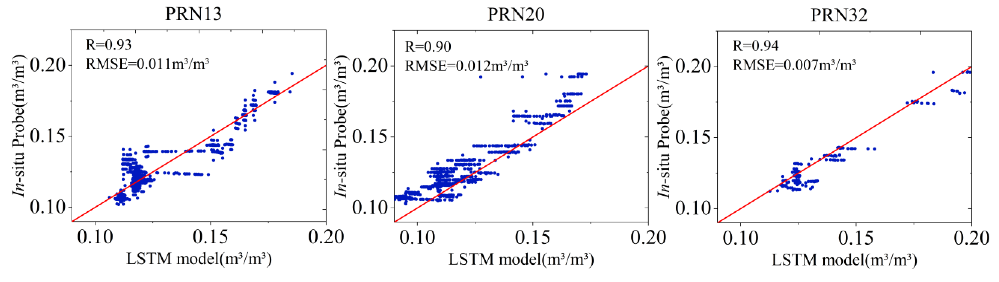
35]. The soil-moisture retrieval experiment using single-satellite data was carried out utilizing 29 satellites. The values of Rrl, TB, and TR at each point in time are used as model inputs for retrieval. Taking PRN13, 20, 32 as an example, the retrieval results from the LSTM model are shown in 
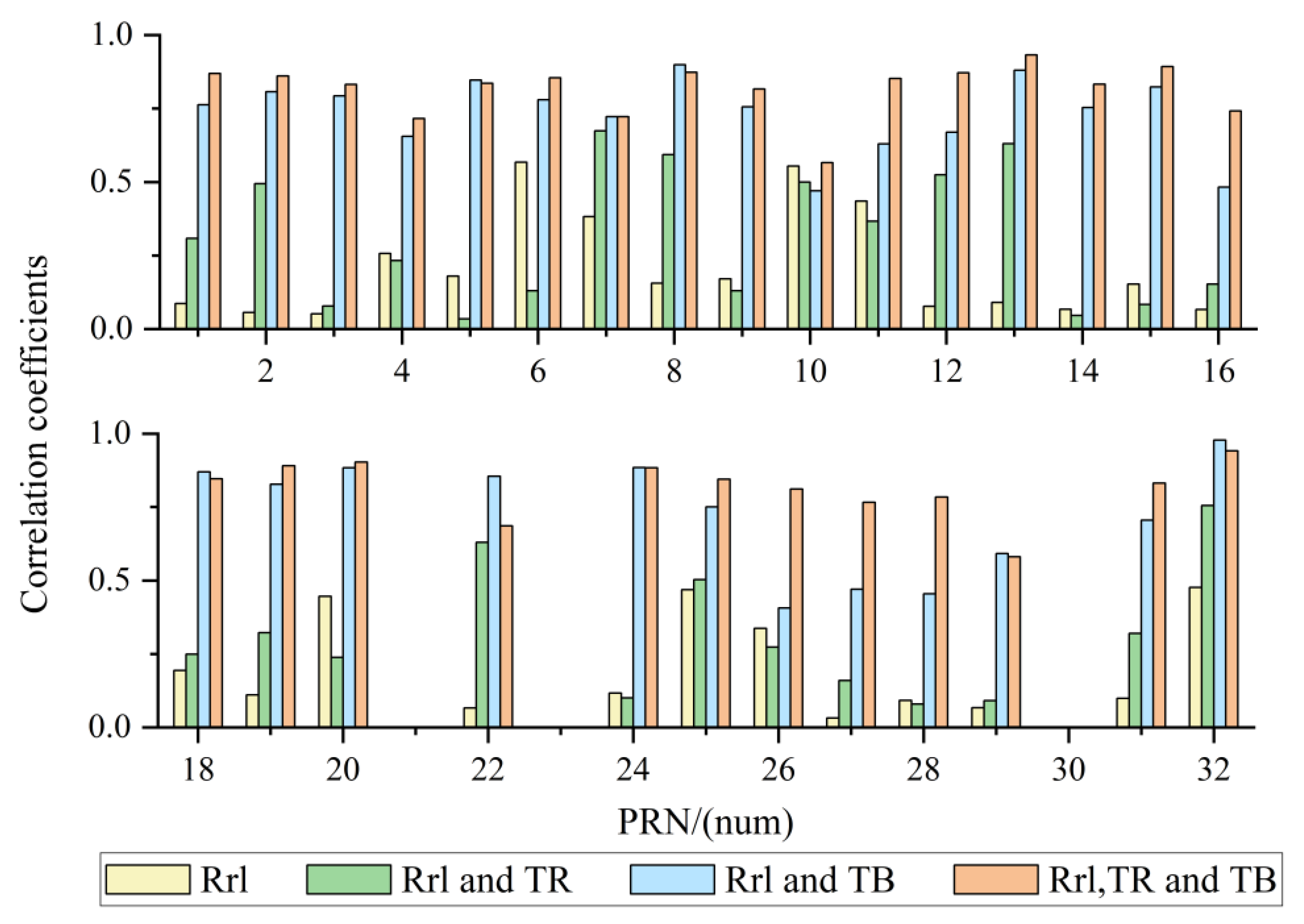
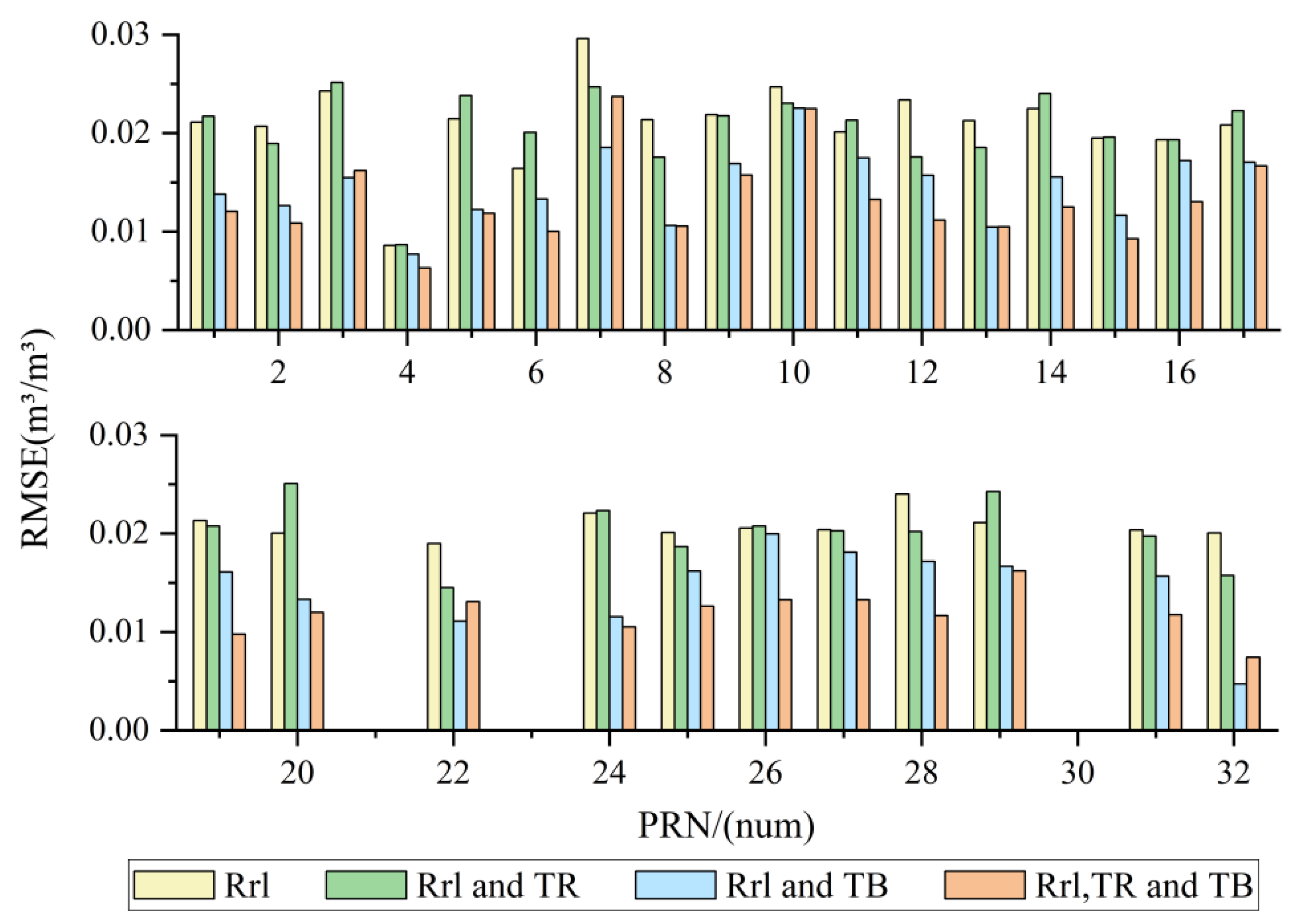
Figure 17, and the retrieval results for all satellites are shown in Figure 18 and Figure 19.
Compared to the Rrl input data alone, the RMSE is reduced by 39 % on average after adding TR and TB, within the set of which PRN32 has the best retrieval effect, with a maximum RMSE reduction of 63%. For demonstration purposes, satellites with a correlation coefficient greater than 0.5 are considered valid for retrieval. We calculated the number of valid satellites for the four configurations. If only reflectivity is used as input, the number of valid satellites is only 2. If TR is added, the number increases to 7. If TB is added, it increases to 24 (Table 8). And when TR and TB are added, all satellites show correlation. However, multiple satellites such as PRN13, 20, and 32 also performed well (R > 0.9). When TR and TB are added, all satellites show correlation (R > 0.5), and the optimum coefficient is 0.94. The single-satellite retrieval statistics show that the model has the highest accuracy after adding two radiometer output products.

4. Discussion

As shown in Figure 11, in this experiment, the retrieval accuracy of the Wang model is poor. Compared to the Wang model, the soil moisture accuracy of ELBARA-II is considerably higher. However, as an experimental prototype, it does not meet the requirements of practical applications. Since the traditional model is strongly affected by noise and does not modify environmental factors such as surface roughness, the retrieval effect improves after average filtering of the results. After averaging the hourly retrieval results, the accuracy of the Wang model improves by 42% and that of the ELBARA-Ⅱ model by 2%. As shown in Figure 12, although the correlation coefficient between the ELBARA-Ⅱ output and the ThetaProbe measurements is high, the RMSE value is still significant. The results show that the trend of ELBARA-Ⅱ is basically consistent with in situ soil moisture, but there is an error in the results. Due to the limited time resolution, the radiometer cannot retrieve soil moisture continuously. Therefore, the LSTM model, which is suitable for continuous time series, is used to retrieve soil moisture.
The model is modified by introducing the auxiliary data TR. When Rrl is used as input data with TR, the RMSE is reduced to 0.018 m³/m³, and the model accuracy improves by 7%. As shown in Figure 20, the prediction error is small under high roughness condition, indicating that TR plays a positive role in correcting the model.
Large-scale precipitation will cause water to accumulate on the surface, which will affect the reception of reflected signals and produce noise. In addition, soil moisture increases sharply, thus affecting model accuracy. There were two precipitation events, 4 April and 8 May 2016, which led to a rapid increase in soil moisture and an abnormal increase in the retrieval accuracy error in these two periods. However, there is a strong negative correlation between TB and soil moisture [26], so auxiliary TB data is introduced to modify the model. When Rrl is used as input with TB, the RMSE is reduced to 0.013 m³/m³, an accuracy improvement of 32%. The correction’s effect is sufficient. Finally, by taking Rrl, TR, and TB together as inputs, the RMSE is further reduced to 0.013 m³/m³, an accuracy improvement of 34% over reflectivity alone as input, indicating that TB plays a positive role in correcting the model.
Since surface roughness, vegetation scattering and other factors affect the accuracy of model retrieval, accuracy can be improved by distinguishing the performance of models with different roughness. When Rrl and TB are used as input data with low roughness, the regression coefficient improves to 0.9, and the RMSE reduces to 0.009, reaching the optimal state. Under these conditions, the model is less affected by roughness, and hardly any roughness correction is required. The time resolution of the TR data output by ELBARA-II is low, so it is necessary to adjust the time scale to the nearest time principle. Therefore, the accuracy reduces when TR is added to the input data. In the case of high roughness, when Rrl, TB, and TR are used as input data at the same time, the correlation coefficient increases from 0.53 to 0.83, the RMSE decreases from 0.009 to 0.007, and the accuracy increases by 27%. It is therefore established that, under high roughness conditions, TR has a good corrective effect on the model.
In the single-satellite soil moisture retrieval experiment, it can be seen that, after adding two types of auxiliary data correction, all satellites become effective satellites, and the correction effect is good. However, only three satellites have a correlation coefficient higher than 0.9. The reason may be that the data from each satellite is getting smaller and smaller, resulting in insufficient data for model training. In future experiments, more data should be considered for single-satellite soil moisture retrieval experiments.

5. Conclusions

In this study, the GNSS-R dual antenna was used for the first time to estimate soil moisture based on the LSTM neural network model. The applicability of the LSTM model for GNSS-R soil moisture retrieval was verified, and the retrieved soil moisture agreed well with the field data. Compared with the in situ probe, the STD of the multi-satellite model was 0.013, which became 0.012 and 0.007 after distinguishing between high and low degrees of roughness, respectively. Moreover, with respect to the single-satellite model, the retrieval results of PRN13, PRN20, and PRN32 were better (R > 0.9), the STD was 0.011, 0.012, and 0.007, respectively, and the temporal resolution was higher than the average of the hourly data obtained by the multi-satellite model. All of the results show that the LSTM model fused with radiometer can reasonably estimate soil moistur compared with the traditional model, it has good noise immunity.
Soil moisture accuracy can be affected by the crosstalk between direct and reflected signals, surface roughness, and vegetation [36]. Assuming that the hourly change of soil moisture is not evident, hourly averaging of reflectivity data will weaken the influences of some environmental factors. However, at the same time, it will also reduce the temporal resolution of the output results. Furthermore, the sampling interval of the radiometer data used here was 6 h, which was quite different from the sampling interval of the GNSS reflectivity data. The matching of the data had to be done according to the nearest-time principle, which limited the correction effect to some extent. In future, we will explore the possibility of using auxiliary data with a higher matching frequency to modify the model, as well as exploring the impact of vegetation and roughness on the model, in order to further improve its accuracy.

Author Contributions

Methodology, C.Y.; Validation, H.N. and B.S.; Writing—original draft, T.Z.; Writing—review & editing, L.Y., X.H. and E.L.-B.; Supervision, D.Y. All authors have read and agreed to the published version of the manuscript.

Funding

This research was funded by National Natural Science Foundation of China, grant number 31971781; Natural Science Foundation Project of Shandong Province, grant number ZR2021MD082; Shanghai Aerospace Science and Technology Innovation Fund, grant number SAST2020-075.

Data Availability Statement

Data sharing is not applicable to this article.

Conflicts of Interest

The authors declare no conflict of interest, and the funders had no role in the design of the study, in the collection, analyses, or interpretation of data, in the writing of the manuscript, or in the decision to publish the results.

References

  1. Engman, E.T. Applications of microwave remote sensing of soil moisture for water resources and agriculture. Remote Sens. Environ. 1991, 35, 213–226. [Google Scholar] [CrossRef]
  2. Le Hegarat-Mascle, S.; Zribi, M.; Alem, F.; Weisse, A.; Loumagne, C. Soil moisture estimation from ERS/SAR data: Toward an operational methodology. IEEE Trans. Geosci. Remote Sens. 2002, 40, 2647–2658. [Google Scholar] [CrossRef]
  3. Kerr, Y.H.; Waldteufel, P.; Wigneron, J.P.; Martinuzzi, J.; Font, J.; Berger, M. Soil moisture retrieval from space: The Soil Moisture and Ocean Salinity (SMOS) mission. IEEE Trans. Geosci. Remote Sens. 2001, 39, 1729–1735. [Google Scholar] [CrossRef]
  4. Loew, A.; Mauser, W. A semiempirical surface backscattering model for bare soil surfaces based on a generalized power law spectrum approach. IEEE Trans. Geosci. Remote Sens. 2006, 44, 1022–1035. [Google Scholar] [CrossRef]
  5. Mattia, F.; Satalino, G.; Dente, L.; Pasquariello, G. Using a priori information to improve soil moisture retrieval from ENVISAT ASAR AP data in semiarid regions. IEEE Trans. Geosci. Remote Sens. 2006, 44, 900–912. [Google Scholar] [CrossRef]
  6. Jiancheng, S.; Wang, J.; Hsu, A.Y.; Neill, P.E.O.; Engman, E.T. Estimation of bare surface soil moisture and surface roughness parameter using L-band SAR image data. IEEE Trans. Geosci. Remote Sens. 1997, 35, 1254–1266. [Google Scholar] [CrossRef]
  7. Hyunglok, K.; Venkat, L. Use of Cyclone Global Navigation Satellite System (CyGNSS) Observations for Estimation of Soil Moisture. Geophys. Res. Lett. 2018, 45, 8272–8282. [Google Scholar]
  8. Munoz-Martin, J.F.; Onrubia, R.; Pascual, D.; Park, H.; Pablos, M.; Camps, A.; Rudiger, C.; Walker, J.; Monerris, A. Single-Pass Soil Moisture Retrieval Using GNSS-R at L1 and L5 Bands: Results from Airborne Experiment. Remote Sens. 2021, 13, 797. [Google Scholar] [CrossRef]
  9. Kavak, A.; Vogel, W.J.; Xu, G. Using GPS to measure ground complex permittivity. Electron. Lett. 1998, 34, 254–255. [Google Scholar] [CrossRef]
  10. Zavorotny, V.; Voronovich, A. Bistatic GPS Signal Reflections at Various Polarisations from Rough Land Surface with Moisture Content. In Proceedings of the IEEE 2000 International Geoscience and Remote Sensing Symposium (IGARSS 2000), Honolulu, HI, USA, 24–28 July 2000; Volume 7, pp. 2852–2854. [Google Scholar]
  11. Zavorotny, V.; Masters, D.; Gasiewski, A.; Bartram, B.; Zamora, R. Seasonal polarimetric measurements of soil moisture using tower-based GPS bistatic radar. In Proceedings of the IEEE International Geoscience & Remote Sensing Symposium, Toulouse, France, 21–25 July 2003. [Google Scholar]
  12. Masters, D.; Axelrad, P.; Katzberg, S. Initial results of land-reflected GPS bistatic radar measurements in SMEX02. Remote Sens. Environ. 2004, 92, 507–520. [Google Scholar] [CrossRef]
  13. Egido, A.; Caparrini, M.; Ruffini, G.; Paloscia, S.; Santi, E.; Guerriero, L.; Pierdicca, N.; Floury, N. Global Navigation Satellite Systems Reflectometry as a Remote Sensing Tool for Agriculture. Remote Sens. 2012, 4, 2356–2372. [Google Scholar] [CrossRef] [Green Version]
  14. Egido, A.; Paloscia, S.; Motte, E.; Guerriero, L.; Pierdicca, N.; Caparrini, M.; Santi, E.; Fontanelli, G.; Floury, N. Airborne GNSS-R Polarimetric Measurements for Soil Moisture and Above-Ground Biomass Estimation. IEEE J. Sel. Top. Appl. Earth Obs. Remote Sens. 2014, 7, 1522–1532. [Google Scholar] [CrossRef]
  15. Yan, Q.; Huang, W.; Jin, S.; Jia, Y. Pan-tropical soil moisture mapping based on a three-layer model from CYGNSS GNSS-R data. Remote Sens. Environ. 2020, 247, 111944. [Google Scholar] [CrossRef]
  16. Wigneron, J.-P.; Kerr, Y.; Philippe, W.; Saleh, K.; Escorihuela, M.J.; Richaume, P.; Ferrazzoli, P.; Rosnay, P.; Gurney, R.; Calvet, J.-C.; et al. L-band Microwave Emission of the Biosphere (L-MEB) Model: Description and calibration against experimental data sets over crop fields. Remote Sens. Environ. 2007, 107, 639–655. [Google Scholar] [CrossRef]
  17. Fernandez-Moran, R.; Wigneron, J.-P.; Lopez-Baeza, E.; Al-Yaari, A.; Coll-Pajaron, A.; Mialon, A.; Miernecki, M.; Parrens, M.; Salgado-Hernanz, P.M.; Schwank, M.; et al. Roughness and vegetation parameterizations at L-band for soil moisture retrievals over a vineyard field. Remote Sens. Environ. Interdiscip. J. 2015, 170, 269–279. [Google Scholar] [CrossRef]
  18. Yin, C.; Lopez-Baeza, E.; Martin-Neira, M.; Fernandez-Moran, R.; Yang, L.; Navarro-Camba, E.A.; Egido, A.; Mollfulleda, A.; Li, W.; Cao, Y.; et al. Intercomparison of Soil Moisture Retrieved from GNSS-R and from Passive L-Band Radiometry at the Valencia Anchor Station. Sensors 2019, 19, 1900. [Google Scholar] [CrossRef] [Green Version]
  19. Goodfellow, I.; Bengio, Y.; Courville, A. Deep Learning; The MIT Press: Cambridge, MA, USA, 2016. [Google Scholar]
  20. Hochreiter, S.; Schmidhuber, J. Long Short-term Memory. Neural Comput. 1997, 9, 1735–1780. [Google Scholar] [CrossRef]
  21. Egido, A. GNSS Reflectometry for Land Remote Sensing Applications. Ph.D. Thesis, Universitat Politècnica de Catalunya, Barcelona, Spain, 2013. [Google Scholar]
  22. Wang, J.R.; Schmugge, T.J. An Empirical Model for the Complex Dielectric Permittivity of Soils as a Function of Water Content. IEEE Trans. Geosci. Remote Sens. 1980, GE-18, 288–295. [Google Scholar] [CrossRef] [Green Version]
  23. Topp, G.C.; Davis, J.L.; Annan, A.P. Electromagnetic determination of soil water content: Measurements in coaxial transmission lines. Water Resour. Res. 1980, 16, 574–582. [Google Scholar] [CrossRef] [Green Version]
  24. Hallikainen, M.T.; Ulaby, F.T.; Dobson, M.C.; El-Rayes, M.A.; Wu, L.K. Microwave Dielectric Behavior of Wet Soil-Part 1: Empirical Models and Experimental Observations. IEEE Trans. Geosci. Remote Sens. 1985, 23, 25–34. [Google Scholar] [CrossRef]
  25. Dobson, M.C.; Ulaby, F.T.; Hallikainen, M.T.; El-rayes, M.A. Microwave Dielectric Behavior of Wet Soil-Part II: Dielectric Mixing Models. IEEE Trans. Geosci. Remote Sens. 1985, GE-23, 35–46. [Google Scholar] [CrossRef]
  26. Schwank, M.; Wiesmann, A.; Werner, C.; Matzler, C.; Weber, D.; Murk, A.; Völksch, I.; Wegmüller, U. ELBARA II, an L-band radiometer system for soil moisture research. Sensors 2010, 10, 584–612. [Google Scholar] [CrossRef] [PubMed] [Green Version]
  27. Fang, K.; Pan, M.; Shen, C. The Value of SMAP for Long-Term Soil Moisture Estimation with the Help of Deep Learning. IEEE Trans. Geosci. Remote Sens. 2019, 57, 2221–2233. [Google Scholar] [CrossRef]
  28. Kratzert, F.; Klotz, D.; Brenner, C.; Schulz, K.; Herrnegger, M. Rainfall–runoff modelling using Long Short-Term Memory (LSTM) networks. Hydrol. Earth Syst. Sci. 2018, 22, 6005–6022. [Google Scholar] [CrossRef] [Green Version]
  29. Yang, T.; Li, B.; Xun, Q. LSTM-Attention-Embedding Model-Based Day-Ahead Prediction of Photovoltaic Power Output Using Bayesian Optimisation. IEEE Access 2019, 7, 171471–171484. [Google Scholar] [CrossRef]
  30. Shahriari, B.; Swersky, K.; Wang, Z.Y.; Adams, R.P.; de Freitas, N. Taking the Human Out of the Loop: A Review of Bayesian Optimisation. Proc. IEEE 2016, 104, 148–175. [Google Scholar] [CrossRef] [Green Version]
  31. Gasmi, A.; Gomez, C.; Chehbouni, A.; Dhiba, D.; El Gharous, M. Using PRISMA Hyperspectral Satellite Imagery and GIS Approaches for Soil Fertility Mapping (FertiMap) in Northern Morocco. Remote Sens. 2022, 14, 4080. [Google Scholar] [CrossRef]
  32. Gebregiorgis, M.; Savage, M. Field, laboratory and estimated soil-water content limits. Water SA 2006, 32, 155–161. [Google Scholar] [CrossRef] [Green Version]
  33. Trifi, M.; Gasmi, A.; Carbone, C.; Majzlan, J.; Nasri, N.; Dermech, M.; Charef, A.; Elfil, H. Machine learning-based prediction of toxic metals concentration in an acid mine drainage environment, northern Tunisia. Environ. Sci. Pollut. Res. 2022, 29, 87490–87508. [Google Scholar] [CrossRef]
  34. Gasmi, A.; Gomez, C.; Chehbouni, A.; Dhiba, D.; Elfil, H. Satellite Multi-Sensor Data Fusion for Soil Clay Mapping Based on the Spectral Index and Spectral Bands Approaches. Remote Sens. 2022, 14, 1103. [Google Scholar] [CrossRef]
  35. Chew, C.C.; Small, E.E.; Larson, K.M.; Zavorotny, V.U. Vegetation Sensing Using GPS-Interferometric Reflectometry: Theoretical Effects of Canopy Parameters on Signal-to-Noise Ratio Data. IEEE Trans. Geosci. Remote Sens. 2015, 53, 2755–2764. [Google Scholar] [CrossRef]
  36. Wang, N.; Gao, F.; Kong, Y.; Xu, T.; Jing, L.; Yang, L.; He, Y.; Yang, W.; Meng, X.; Ning, B. Soil Moisture Estimation Based on GNSS-R Using L5 Signals from a Quasi-Zenith Satellite System. IEEE Geosci. Remote Sens. Lett. 2022, 19, 2505005. [Google Scholar] [CrossRef]
Figure 1. GNSS-R scattering geometry.
Remotesensing 15 02693 g001
Figure 2. Schematic diagram of GNSS-R soil moisture retrieval.
Remotesensing 15 02693 g002
Figure 3. The three ELBARA-II prototype systems at the test site at the Swiss Federal Research Institute WSL [26]. Reprinted/adapted with permission from Ref. [26]. 2010, Schwank, M.; Wiesmann, A.; Werner, C.; Matzler, C.; Weber, D.; Murk, A.; Völksch, I.; Wegmüller, U.
Remotesensing 15 02693 g003
Figure 4. LSTM neuron structure diagram.
Remotesensing 15 02693 g004
Figure 5. LSTM structure diagram.
Remotesensing 15 02693 g005
Figure 6. Oceanpal antenna and calibration box.
Remotesensing 15 02693 g006
Figure 7. Schematic diagram of the Valencia experimental site.
Remotesensing 15 02693 g007
Figure 8. Soil moisture ThetaProbe sensors and the Davis Vantage Pro 2 meteorological station.
Remotesensing 15 02693 g008
Figure 9. LHCP reflectivity vs. elevation angle.
Remotesensing 15 02693 g009
Figure 10. Data processing workflow.
Remotesensing 15 02693 g010
Figure 11. Retrieval results of Wang model and ELBARA-Ⅱ.
Remotesensing 15 02693 g011
Figure 12. Retrieval results of the Wang model and the ELBARA-Ⅱ radiometer (averaged in hours).
Remotesensing 15 02693 g012
Figure 13. Soil moisture estimation results of the LSTM model optionally using different input data.
Remotesensing 15 02693 g013
Figure 14. TR data of October 2014–June 2016.
Remotesensing 15 02693 g014
Figure 15. Soil moisture estimation results of the LSTM model with low roughness conditions.
Remotesensing 15 02693 g015
Figure 16. Soil moisture estimation results of the LSTM model under high-roughness conditions.
Remotesensing 15 02693 g016
Figure 17. Retrieval results from the LSTM model taking Rrl, TR and TB as inputs (PRN 13, 20, 32).
Remotesensing 15 02693 g017
Figure 18. Correlation coefficients for the four configurations between Rrl, TR and TB.
Remotesensing 15 02693 g018
Figure 19. RMSE for the four configurations between Rrl, TR, and TB.
Remotesensing 15 02693 g019
Figure 20. Prediction error of the LSTM model under high-roughness conditions.
Remotesensing 15 02693 g020
Table 1. Statistical errors between retrieved soil moisture and in situ measurements.
RRMSE (m³/m³)
Wang model0.090.123
ELBARA-Ⅱ0.580.101
Corrected ELBARA-Ⅱ0.780.024
Table 2. Statistical errors between retrieved soil moisture and in situ measurements.
RRMSE (m³/m³)
Wang model0.260.087
ELBARA-Ⅱ0.830.098
Corrected ELBARA-Ⅱ0.830.024
Table 3. Statistical errors between retrieved soil moisture and in situ measurements.
RRMSE (m³/m³)
Rrl as input0.500.019
Rrl, TR as input0.580.018
Rrl, TB as input0.810.013
Rrl, TB and TR as input0.830.013
Table 4. Statistical errors of different methods of allocating data.
RRMSE (m³/m³)
80%, 20%0.800.013
70%, 30%0.830.013
60%, 40%0.710.015
Table 5. Statistical errors of MLP-BP and the SVM model.
RRMSE (m³/m³)
MLP-BP0.370.023
SVM0.690.017
LSTM0.830.013
Table 6. Statistical errors between retrieved soil moisture and in situ measurements.
RRMSE (m³/m³)
Rrl, TR as input0.670.017
Rrl, TB as input0.900.009
Rrl, TB and TR as input0.850.012
Table 7. Statistical errors between retrieved soil moisture and in situ measurements.
RRMSE (m³/m³)
Rrl, TR as input0.360.010
Rrl, TB as input0.530.009
Rrl, TB and TR as input0.830.007
Table 8. Number of effective satellites used with different input data.
R > 0.5
Rrl as input2
Rrl, TR as input7
Rrl, TB as input24
Disclaimer/Publisher’s Note: The statements, opinions and data contained in all publications are solely those of the individual author(s) and contributor(s) and not of MDPI and/or the editor(s). MDPI and/or the editor(s) disclaim responsibility for any injury to people or property resulting from any ideas, methods, instructions or products referred to in the content.

