Article

A Novel Edge Detection Method for Multi-Temporal PolSAR Images Based on the SIRV Model and a SDAN-Based 3D Gaussian-like Kernel

High-Tech Institute of Xi’an, Xi’an 710025, China
*
Author to whom correspondence should be addressed.
Remote Sens. 2023, 15(10), 2685; https://doi.org/10.3390/rs15102685
Submission received: 9 March 2023 / Revised: 8 May 2023 / Accepted: 18 May 2023 / Published: 22 May 2023
(This article belongs to the Special Issue Advances of SAR Data Applications)

Abstract

:
Edge detection for PolSAR images has demonstrated its importance in various applications such as segmentation and classification. Although there are many edge detectors which have demonstrated an impressive ability to achieve accurate edge detection results, these methods only focus on edge detection in a single-date PolSAR image. However, a single-date PolSAR image cannot fully characterize the changes in scattering mechanisms of land cover in different growth cycles, resulting in some omissions of the true edges. In this paper, we propose a novel edge detection method for multi-temporal PolSAR images based on the SIRV model and an SDAN-based 3D Gaussian-like kernel. The spherically invariant random vector (SIRV) and span-driven adaptive neighborhood (SDAN) improve the estimation accuracy of the average covariance matrix (ACM) in terms of data representation and spatial support, respectively. We propose an SDAN-based 2D Gaussian kernel to accurately extract the edge strength of single-date PolSAR images. Then, we design a 1D convolution kernel in the temporal dimension to smooth fluctuations in the edge strength of multi-temporal PolSAR images. The SDAN-based 2D Gaussian kernels in the X- and Y-directions are combined with the 1D convolution kernel in the Z-direction to form an SDAN-based 3D Gaussian-like kernel. In addition, we design an adaptive hysteresis threshold method to optimize the edge map. The performance of our proposed method is presented and analyzed on two real multi-temporal PolSAR datasets, and the results demonstrate that the proposed edge detector achieves a better performance than other edge detectors, particularly for crop regions with time-varying scattering mechanisms.

1. Introduction

Polarimetric synthetic aperture radar (PolSAR) has received increasingly more attention due to its capability to provide unique and useful information and has been widely used in various applications [1]. As a prerequisite step for PolSAR image processing and interpretation, edge detection of PolSAR images is very important, which can provide crucial structural information for superpixel segmentation [2] and speckle noise reduction [3], as well as land cover classification [4] and change detection [5].
PolSAR image edge detection is still a challenging task due to the inherent speckle noise. To solve this problem, an effective method is to estimate the average covariance matrix within the window on both sides of the central pixel using a bi-window filter. Schou et al. [6] firstly proposed an original PolSAR edge detector, which visits each pixel in sequence and extracts the edge information using a classic rectangle window with different orientations. Inspired by this, Shui et al. [7] proposed a Gaussian-Gamma-shaped (GGS) filter instead of the rectangular filter, which can reduce false-edge pixels near true edges. Xiang et al. [8] proposed a Gaussian-shaped (GS) filter instead of the rectangular filter, giving a larger weight to the center pixel. Wang et al. [9] further proposd an enhanced edge detection method for PolSAR data based on the directional span-driven adaptive window, which can overcome the limitations of classic fixed-shape windows and achieve better edge detection results than the Gaussian-shaped window. Jin et al. [10] proposed a nonsubsampled contourlet transform for PolSAR image edge detection, which can provide flexible multiscale and directional decomposition. Sharma et al. [11] proposed a patch-based NLM adaptive speckle filter based on a constant false alarm rate edge detector, which can reduce the effect of speckle noise on edge detection results. Deng et al. [12] proposed an edge detector for PolSAR images based on a polarimetric whitening filter which can enhance the continuity of the detected edges by exploiting the correlation between the different polarization channels.
In addition, an accurate estimation of the covariance matrix and its distance metric can likewise affect the accuracy of edge detection. Nascimento et al. [13] compared the effectiveness of four stochastic distances, two differences of entropies, and the maximum likelihood criterion for PolSAR image edge detection. De et al. [14] proposed an edge detection method based on fusing the evidences obtained in the intensity channels HH, HV, and VV of PolSAR images, which contains a simple average, multi-resolution discrete wavelet transform, a principal component analysis, ROC statistics, a multi-resolution stationary wavelet transform, and a multi-resolution method based on singular value decomposition. Shi et al. [15] fused a constant false alarm edge detector and a weighted gradient edge detector to detect both strong and weak edges. Most of these methods are proposed under the assumption of the complex Wishart distribution; however, in heterogeneous regions, this assumption is usually not appropriate [16]. In PolSAR images, edge pixels are often considered heterogeneous due to the change in scattering mechanisms between different land cover classes, which leads to non-Gaussian clutter modeling [17]. A commonly used PolSAR non-Gaussian clutter model is the product model, i.e., modelling the clutter as the product between the square root of a scalar random variable and an independent zero-mean complex circular Gaussian random vector [18]. Yao et al. [19] proposed spherically invariant random vectors (SIRV), which are a class of non-homogeneous Gaussian processes with random variance. Xiang et al. [8] introduced a SIRV into the PolSAR edge detection algorithm and demonstrated the superiority of this SIRV model in modeling heterogeneous regions.
Although the above methods improve the PolSAR edge detection method using various aspects such as the statistical distribution model, bi-window shapes, and joint edge detectors, they all perform edge detection on a single-date PolSAR image. However, for land covers with time-varying scattering mechanisms (e.g., vegetation and crops), different land covers may exhibit similar scattering mechanisms in a single-date PolSAR image, making it difficult to extract the edges of these land covers. As shown in Figure 1, in PolSAR images with two dates, there is not only overlapping edge information, but also complementary edge information. Multi-temporal PolSAR images can fully describe the changes in scattering mechanisms of crops in different growth cycles, as shown in the red dotted circles in the figure. However, state-of-the-art edge detection algorithms have been developed based on single-date PolSAR images, and are not suitable for edge detection of multi-temporal PolSAR images. At present, there are only a few studies on multi-temporal PolSAR image edge detection. Generally, for multi-temporal PolSAR image edge detection, researchers first implement edge detection of a single-date PolSAR image using the above 2D bi-window filters (also referred to as 2D convolution kernels) and then perform simple 1D filters (also referred to as 1D convolution kernels) in the temporal dimension, such as the mean kernel, maximum kernel, minimum kernel, and root mean square (RMS) kernel [20]. However, the maximum kernel may obtain many false edges within the land plot, whereas the minimum kernel may lose a lot of true edges. The mean kernel may not detect some weak edges. The RMS kernel amplifies the sensitivity to timing variations, but also increases the interference of speckle noise in the edge detection results. Therefore, it is necessary to develop a 1D kernel in the temporal dimension that can effectively extract both strong and weak edges and suppress the effects of speckle noise.
In this paper, we propose a novel edge detection method for multi-temporal PolSAR images based on the SIRV model and an SDAN-based 3D Gaussian-like kernel. Specifically, to accommodate the complex distribution of heterogeneous regions, the SIRV model is used instead of the Wishart distribution model to describe the back-scattering statistics of PolSAR images. Then, under the SIRV model, a maximum likelihood distance is defined to measure the distance between the normalized covariance matrices. We define a 3D Gaussian-like kernel to convolve the multi-temporal PolSAR images to obtain an edge strength map (ESM). Strictly speaking, this kernel is not a standard 3D Gaussian kernel function in a 3D space, but a 2D Gaussian kernel in X- and Y-directions and a 1D convolution kernel in the temporal dimension direction (henceforth called the Z-direction). We define a new 1D convolution kernel in the Z-direction to smooth the edge strength fluctuations between multi-temporal PolSAR images due to variations in scattering information. Due to the multi-scale characteristics of land covers, fixed-size bi-windows (e.g., rectangular-shaped, GS-shaped, and GGS-shaped) make it difficult to ensure that the window contains only homogeneous pixels, thus reducing estimation accuracy. Therefore, the span-driven adaptive neighborhood (SDAN) is adopted as the 2D spatial support, which can obtain a bi-window with a flexible shape and variable size. Then, the SDAN is combined with the 3D Gaussian-like kernel to form an SDAN-based 3D Gaussian-like kernel, which is used to obtain an accurate ESM. Finally, the non-maximum suppression (NMS) strategy is used on the ESM of multi-temporal PolSAR images, followed by an adaptive hysteresis threshold method to optimize the edge detection results. The experimental results on two sets of multi-temporal PolSAR images show that our proposed edge detection method outperforms other state-of-the-art methods.
The rest of this paper is organized as follows. In Section 2, the proposed method is introduced. Section 3 gives the experimental results of our proposed method as well as comparisons with other state-of-the-art methods. Finally, the conclusions are given in Section 4.

2. Methodology

Schou et al. [6] proposed the classical bi-window edge detection framework, which uses rectangular windows on either side of the central pixel to calculate the average covariance matrices (ACMs) and uses the distance between the ACMs as a measure of edge probability. Although this method has been widely used for edge detection of various PolSAR images, it still has three limitations, as follows.
(1)
The Wishart distribution is not suitable for heterogeneous regions of PolSAR images, thus failing to accurately estimate the ACM.
(2)
The rectangular window does not ensure all internal pixels are homogeneous, which also leads to an inaccurate ACM estimation.
(3)
The rectangular kernel assigns equal weight to all pixels, which ignores the important fact that the information contained in the pixels near the centre pixel is more important than that at other pixels.
(4)
The method requires the use of hysteresis thresholds to eliminate noise edges, and the values of the hysteresis thresholds usually need to be adjusted repeatedly by experiment, increasing the difficulty of hyperparameter estimation.
Figure 2 gives the overall architecture of the proposed method. The proposed method consists of four important parts, i.e., SIRV-based PolSAR representation, SDAN-based spatial support, a 3D Gaussian-like kernel, and an adaptive hysteresis threshold. Firstly, the SIRV model is used to replace the Wishart distribution model, thereby improving the accuracy of covariance matrix estimation in complex edge regions. Secondly, we adopt the SDAN as a spatial support to search for homogeneous regions on both sides of the central pixel as the regions for ACM estimation. Thirdly, we propose a 3D Gaussian-like kernel to convolve the multi-temporal PolSAR images, which can smooth the edge strength fluctuations between multi-temporal PolSAR images. Then, the SDAN is combined with the 3D Gaussian-like kernel to form an SDAN-based 3D Gaussian-like kernel, which is used to extract an accurate ESM. Finally, we propose an estimation method for hysteresis thresholds, which reduces the number of hyperparameters in the edge detection algorithm and improves the practicality of the method. In this section, we will introduce the details and contributions of the four modules.

2.1. SIRV-Based PolSAR Representation

In the polarization observation, the target vector k can be usually constructed with the Pauli bases as [21]
k = 1 2 S H H + S V V , S H H S V V , 2 S H V T ,
where S H H , S H V , and S V V are the elements of a complex scattering matrix S. In the case of satisfying the reciprocity theorem and single station backscatter, the covariance matrix C of PolSAR data can be defined as
C = S H H 2 2 S H H S H V * S H H S V V * 2 S H V S H H * 2 S H V 2 2 S H V S V V * S V V S H H * 2 S V V S H V * S V V 2
Although a complex Wishart distribution is widely used for the statistical modeling of the multilooked covariance matrix C, this distribution is usually violated in heterogeneous regions of PolSAR images [22]. The SIRV model can describe a class of entire stochastic distributions [19], which would be suitable for the heterogeneous areas of PolSAR data. Therefore, the SIRV model can be considered for edge detection. It defines the m-dimensional complex measurement k as the product between the independent complex circular Gaussian vector z (speckle) and the square root of the positive random variable τ (texture):
k = τ z .
For PolSAR data interpretation, the normalized covariance matrix C could be used to denote polarimetric diversity and τ can be considered as the spatial texture. Thus, the probability density function (PDF) of k can be written as
P D F ( k τ , C ) = 1 ( π ) m N | C | N i = 1 N 1 τ i m exp k i C 1 k i τ i ,
where the superscript † denotes the conjugate transpose. N denotes the number of independent data used in the estimation. In this paper, m = 3 . Then, the texture estimator τ ^ i can be calculated by maximizing the log-likelihood function of Equation (4) as
τ ^ i = k i C 1 k i m .
Then, substituting Equation (5) into Equation (4), we can obtain the maximum-likelihood estimator of the covariance matrix as
C ^ = f ( C ^ ) = m N i = 1 N k i k i k i C ^ 1 k i
which can be implemented in a fixed point recursive way, i.e., C ^ i + 1 = f ( C ^ i ) . More details on the estimation algorithm can be found in [18].

2.2. SDAN-Based Spatial Support

In the estimation of ACMs for complex regions, it is difficult to ensure that the pixels within a rectangular window are all homogeneous, as shown in Figure 3a. Although researchers have proposed window shapes such as GS and GGS to increase the weight of pixels close to the centre, they still cannot completely solve the problem of inaccurate ACM estimation in heterogeneous regions. SDAN has been widely used as an adaptive neighbourhood search strategy for PolSAR image interpretation [23,24]. As shown in Figure 3b, for a given initial seed region of size 2 × 3 , an SDAN window is generated by a region growth method. Firstly, an unbiased estimate of the seed span value is calculated using the initial seed region, which can be written as
p ^ s = p ¯ r + b p s p ¯ r , b = var p r p ¯ r 2 σ n 2 var p r 1 + σ n 2
where p ^ s denotes the unbiased estimate of the seed span value. p ¯ r and var p r denote the mean and variance values of the initial seed region span, respectively. σ n 2 denotes the variance of the system noise. SDAN uses two symmetric confidence intervals to select spatially contiguous pixels as adaptive neighbours, which can be expressed as
( i , j ) A N , i f p ( i , j ) p ^ s [ 1 δ , 1 + δ ] ( i , j ) A N , o t h e r w i s e
where ( i , j ) denotes a direct neighbor of the initial seed region. A N denotes an adaptive neighbourhood. δ denotes the confidence coefficient. The growing procedure is iteratively applied for all neighbors of the pixels in A N until none of the new neighbors fulfil the condition or the upper limit of the number of neighbours N is reached.

2.3. SDAN-Based 3D Gaussian-like Kernel

In this paper, we propose an SDAN-based 3D Gaussian-like kernel to convolve multi-temporal PolSAR images to obtain accurate ESMs. Strictly speaking, this kernel is not a standard 3D Gaussian kernel function in a 3D space, but a 2D Gaussian kernel in X- and Y-directions and a 1D convolution kernel in the Z-direction. The 2D Gaussian kernel can be written as
W ( x , y ) = 1 2 π σ x 2 π σ y exp x 2 2 σ x 2 + y 2 2 σ y 2
where σ x and σ y control the GS window length and width, respectively. In this paper, we use the SDAN as a spatial support and combine the SDAN with the 2D Gaussian kernel, so that the size of the 2D Gaussian kernel is calculated as the minimum external GS window of the SDAN. Therefore, the SDAN-based 2D Gaussian kernel is written as
W A N ( x , y ) = W ( x , y ) × A N ( x , y ) , A N ( x , y ) = 1 , ( x , y ) A N 0 , ( x , y ) A N
Then, the average covariance matrix M obtained by the SDAN-based 2D Gaussian kernel can be calculated as
M = ( x , y ) W A N ( x , y ) C ^ ( x , y ) ( x , y ) W A N ( x , y ) .
The distance between M 1 and M 2 can be calculated as
D M 1 , M 2 = ln M 1 M 2 + m N i = 1 N k i M 1 1 k i k i M 2 1 k i .
Next, we give the definition of the 1D convolution kernel in the Z-direction given the distance ( D 1 D t ) between two ACMs of the central pixel in the X- and Y-directions. The 1D convolution kernel ( K = [ β 1 β t ] ) is defined as
β i = n o r m C o V i C o V , i 1 t
in which,
C o V = σ μ , μ = 1 t k = 1 t D k , σ = 1 t k = 1 t D k μ 2 C o V i = σ i μ i , μ i = 1 t 1 k = 1 , k i t D k , σ i = 1 t 1 k = 1 , k i t D k μ i 2
The coefficient of variation (CoV) provides a better measure of the variation in the ACM distance in the temporal dimension. It can be seen by (13) that the greater the change in ACM distance of the i-th temporal PolSAR image, the smaller β i . Thus, the 1D convolution kernel smooths edge strength variations in the temporal dimension and reduces false edge pixels caused by speckle noise. Then, the SDAN-based 3D Gaussian-like kernel can be defined as
G = K × W A N × K T
Now, the multi-temporal average covariance matrix T obtained by the SDAN-based 3D Gaussian-like kernel can be calculated as
T = ( x , y ) A N z [ 1 t ] G ( x , y , z ) · C ^ m ( x , y , z ) ( x , y ) A N z [ 1 t ] G ( x , y , z )
where C ^ m denotes stacking of multi-temporal maximum likelihood covariance matrices, i.e., C ^ m = C ^ 1 ; ; C ^ t .
The distance between T 1 and T 2 can be calculated as
D T 1 , T 2 = ln T 1 T 2 + m N i = 1 N k i T 1 1 k i k i T 2 1 k i .
Finally, the edge strength map, E S M , of multi-temporal PolSAR images can be calculated as
E S M = m a x θ { D ( T 1 , T 2 | θ ) }
where θ denotes the orientation angle.

2.4. Adaptive Hysteresis Threshold

Once the ESM is obtained, the NMS is usually used to eliminate redundant edges. However, the edge results after non-maximum suppression processing still have many noisy edges, which need to be optimized by the hysteresis thresholds. The hysteresis thresholds contain two thresholds, i.e., the high threshold T h i g h and the low threshold T l o w , which are generally adjusted repeatedly through experiments [25]. However, manual determination of hysteresis thresholds is time consuming. Although many researchers have reduced the parameter search time by establishing range of optimal thresholds, edge detection results depend on the range of optimal thresholds [26,27]. Therefore, we propose a simple and effective method for estimating hysteresis thresholds. We noticed that the number of edge positions is much less than that of non-edge positions in most scenes, and the probability density of non-edges is much greater than that of edges. Moreover, we can observe from Figure 4 that the probability density function (PDF) of the ESM is similar to the chi-square distribution, which has been approximatively used in this paper to fit the PDF of the ESM.
Therefore, we fit the ESM to a chi-square distribution function as
f ( x ) = 1 2 k 2 Γ k 2 x k 2 1 e x 2 , x 0 0 , x < 0
Then, we calculate the value for which the derivative of (19) is 0, which is taken as the low threshold.
f ( x ) = 1 2 k 2 Γ k 2 k 2 1 x k 2 2 e x 2 1 2 x k 2 1 e x 2 = 0 k 2 1 x k 2 2 e x 2 1 2 x k 2 1 e x 2 = 0 x = k 2 2
where k is the freedom degree of the chi-square distribution, which can be obtained by fitting the ESM. Now, T l o w and T h i g h can be obtained by [8,28]
T l o w = k 2 2
T h i g h = T l o w + 0.02 n , n = [ 1 , 2 , . . . , ( 0.4 T l o w ) / 0.02 ]

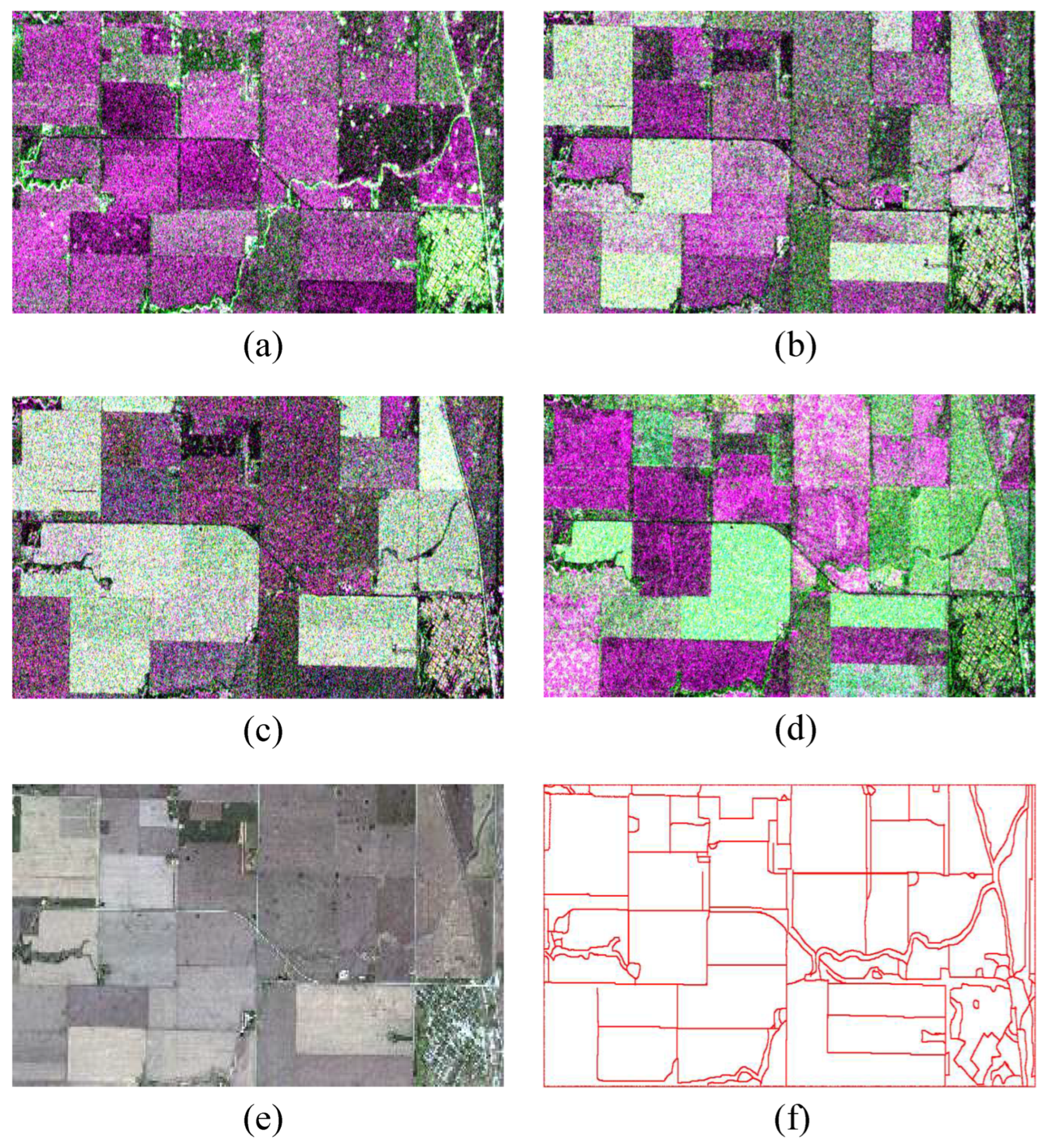
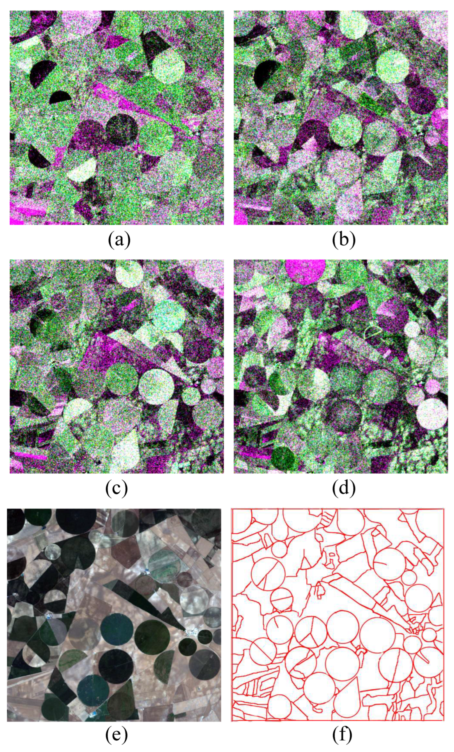
3. Experimental Results

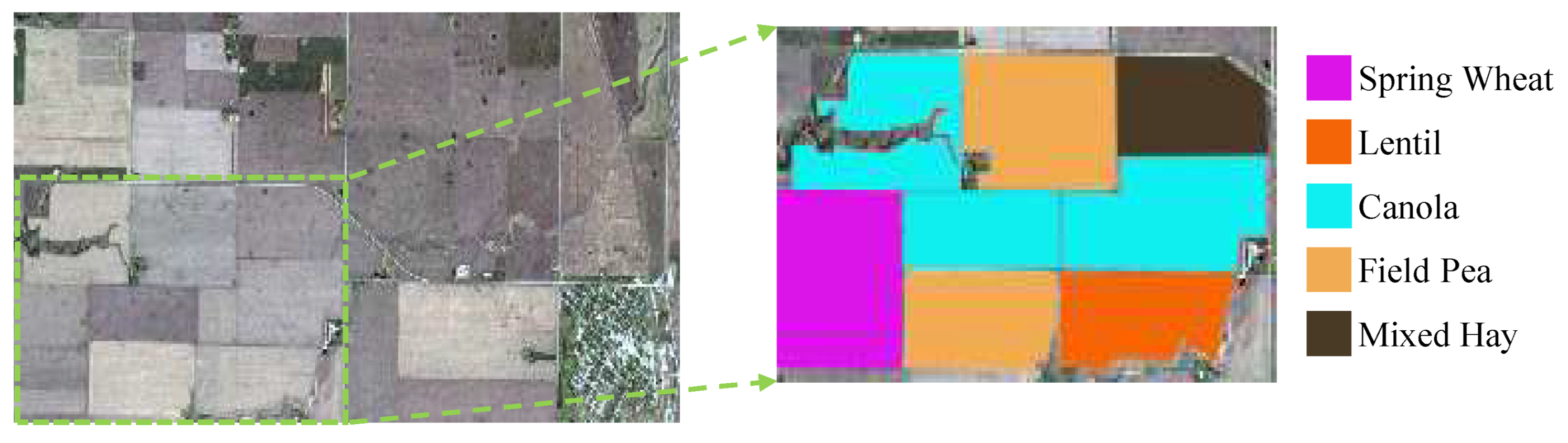
3.1. Data Description and Parameter Settings

To demonstrate the effectiveness of our proposed method, we chose two multi-temporal PolSAR datasets for evaluation. The two multi-temporal PolSAR image datasets were acquired by the RADARSAT-2 C-band system with the study areas located in India Head ( 50.34 ° N, 103.36 ° W), Canada, and Barrax ( 39.51 ° N, 2.14 ° W), Spain. These images are from the AgriSAR 2009 Campaign project supported by the European Space Agency. The experimental datasets are quad-polarimetric SAR datasets, which consist of HH, HV, VH, and VV channels. The resolution is 5.4 m × 8.0 m (range × azimuth). The incidence angle is approximately 20 ° at the near range and 41 ° at the far range. The size of the Indian Head dataset is 450 × 1000, and pseudo color images formed by PauliRGB decomposition are shown in Figure 5. The azimuth and range directions of the Indian Head dataset are shown in the Pauli image. The PauliRGB decomposition images of Barrax dataset are shown in Figure 6. The azimuth and range directions of are shown in the figure. In addition, it is important to note that each multi-temporal PolSAR dataset was acquired in the same satellite orbit. The ground truth edges are obtained from the corresponding multi-temporal optical images.
In our experiments, the maximum number of neighbours N was set to 20. The confidence coefficient δ was set to 3. The orientation angle θ was discredited into θ = 0 π / 8 , , 7 π / 8 . The size of the 1D convolution kernel was equal to the number of multi-temporal PolSAR images. Since we designed an adaptive hysteresis threshold method, the number of parameters of our proposed method is less than that of other methods. To verify the effectiveness of the proposed method, we implement different 2D convolution kernels and 1D convolution kernels for comparison experiments.

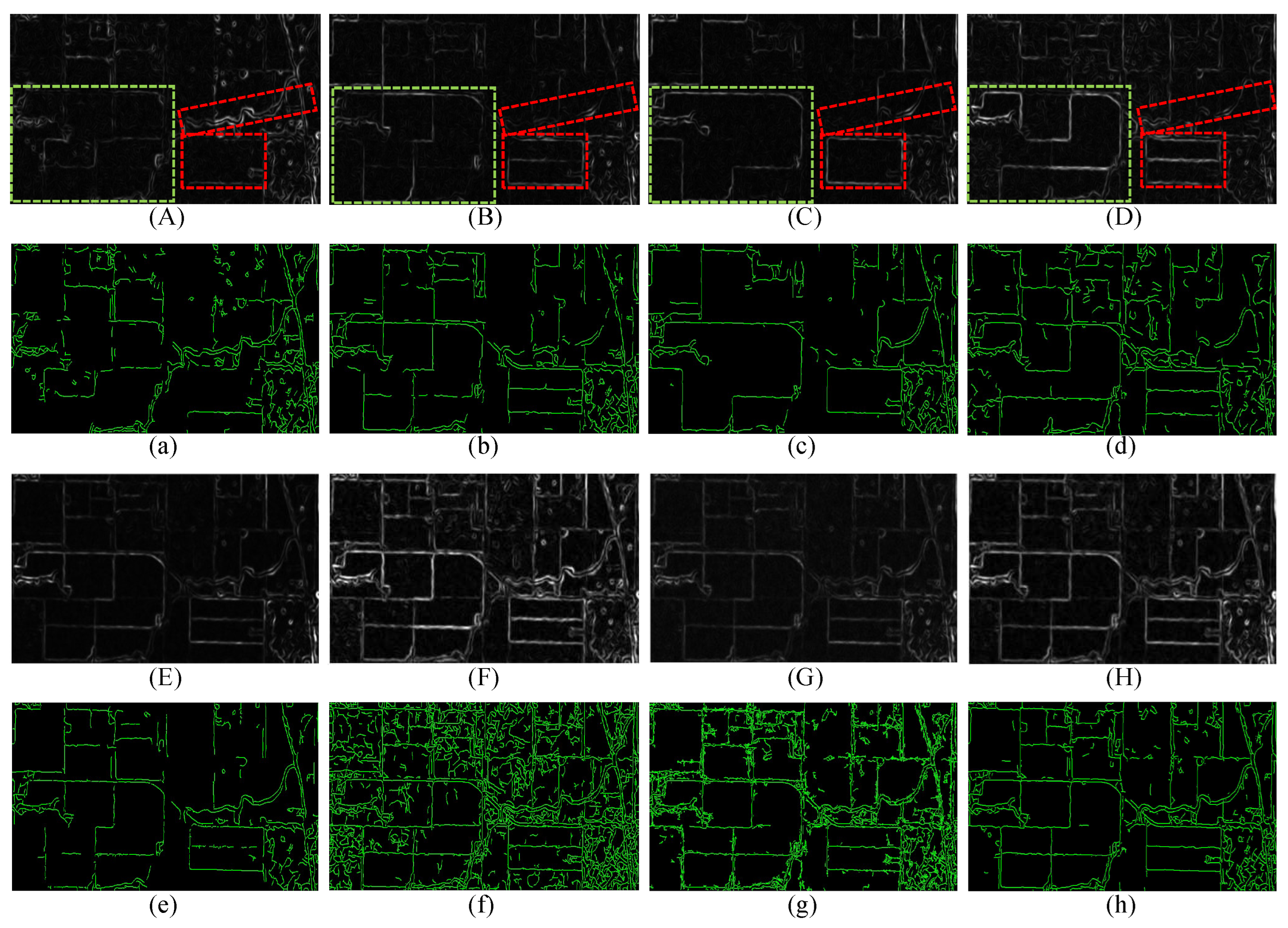
3.2. Edge Detection Reuslts

As mentioned earlier, the proposed 3D Gaussian-like kernel is not a standard 3D Gaussian kernel in 3D space, but consists of the SDAN-based 2D Gaussian kernel and a 1D convolution kernel. Therefore, to investigate the effectiveness of the proposed 1D convolution kernel in multi-temporal PolSAR image edge detection, we designed several sets of comparison experiments. In the comparison experiments, we used the same SDAN-based 2D Gaussian kernel as the convolution kernel in the X- and Y-directions, and formed 3D convolution kernels with different 1D convolution kernels in the Z-direction. The three 1D convolution kernels used for comparison contain the mean kernel ( K m e a n ), the maximum kernel ( K m a x ), and the root mean square (RMS) kernel ( K R M S ), which are defined as
K m e a n = [ α 1 , , α t ] , α i = 1 t
K max = [ ε 1 , , ε t ] , ε i = 1 , i = arg max ( D i ) 0 , o t h e r w i s e
K R M S = [ ω 1 , , ω t ] , ω i = D i 2 j D j 2
where D i is calculated from (12). The 3D convolution kernels used for comparison are called the 3D mean kernel, the 3D maximum kernel, and the 3D RMS kernel, respectively.
The ESMs and edge maps obtained by different 3D kernels are shown in Figure 7. From Figure 7a–d, we can observe that it is not possible to detect complete edges on the single-date PolSAR image, and the edge detection results of the PolSAR image of four dates complement each other, especially in the regions marked by green and red boxes. For example, in the result on 23 April, most of the road edges can be detected, but the crop edges are poorly detected. However, in the results on 17 May, 10 June, and 12 September, only a small number of road edges are detected. This result reconfirms the necessity of using multi-temporal PolSAR images for edge detection.
Here, we give a specific example to explain the reason for the results. The region marked by a green box in Figure 7A–D contains Spring Wheat, Field Pea, Canola, Lentil, and Mixed Hay, as shown in Figure 8, all of which have different growth cycles and time-varying scattering mechanisms. Figure 9 shows photographs of Field Pea and Canola developments. We can observe that Field Pea and Canola do not cover the surrounding land and their scattering mechanisms are close to that of the arable land in the seeding stage and the early stage of development. In the peak stage of development, both Field Pea and Canola have dense branches and leaves, which exhibit strong volume scattering power, resulting in a failure of edge detection between the two crops, as shown in Figure 7c. In the late stage of development, the growth status of Field Pea and Canola show a huge difference, and the scattering mechanisms of their edges are also significantly different. Therefore, clear edges between the two crops can be detected on 12 September, as shown in Figure 7d. The above analyses further illustrate the necessity of using multi-temporal PolSAR images to achieve edge detection.
As shown in Figure 7e, the 3D mean kernel can reduce false edges caused by speckle noise, it will miss many weak edges. In contrast, the 3D maximum kernel is able to completely detect strong and weak edges, but its result contains a large number of false edges, as shown in Figure 7f. The 3D RMS kernel is effective in detecting weak edges and reducing the number of false edges, but there are still some pixels near real edges that are incorrectly detected as edges, as shown in Figure 7g. However, our proposed method can effectively reduce the generation of false edges and detect relatively complete edges, as shown in Figure 7h. In terms of running time, although the 3D RMS kernel and the 3D Gaussian-like kernel require additional computation of the convolution kernel in the Z-direction, the computational complexity of this operation is extremely low and the running time is negligible.
Correspondingly, we present the quantitative comparison results of the Indian Head dataset with different methods, as listed in Table 1. We can find that the recall of single-date PolSAR image detection results is fairly low, indicating that a large number of edges are not detected. Although the recall of the edge detection result on 12 September is high, its precision is only 0.58, indicating that there are many false edges in the edge detection result. After convolving the multi-temporal PolSAR images with the 3D mean kernel, the precision of the edge detection result is significantly improved, but its recall is even lower than that of the 12 September edge detection result. In contrast, the edge detection result with the 3D maximum kernel has a higher recall but lower precision. Compared to the 3D maximum kernel, the 3D RMS kernel significantly reduces the number of false edges and improves the precision by 0.21. However, the proposed method achieves the highest precision while maintaining a high recall.
Figure 10 shows the edge maps of the Barrax dataset obtained by different methods, where the same observations can be made as the Indian Head dataset. It can be seen from Figure 10a–d that a single-date PolSAR image cannot detect complete edges. The 3D mean kernel can significantly reduce the number of false edges, whereas many weak edges are ignored, as shown in Figure 10e. The 3D maximum kernel is able to detect complete edges, whereas many false edges within the land cover are incorrectly detected, as shown in Figure 10f. Compared to the 3D maximum kernel, the 3D RMS kernel can further reduce the occurrence of false edges, as shown in Figure 10g. Compared to other methods, our proposed SDAN-based 3D Gaussian-like kernel can further reduce the number of false edges and maximise the retention of true edges, as shown in Figure 10h.
Correspondingly, we present the quantitative comparison results of the Barrax dataset with different methods, listed in Table 2. The edge detection results of the single-date PolSAR image vary with different crop growth changes and do not detect complete edges. According to the recall of the edge detection results, it can be seen that multi-temporal PolSAR images give more complete edges than the single-date PolSAR image. The 3D mean kernel obtains the lowest recall. The 3D maximum kernel obtains the lowest precision. Our proposed SDAN-based 3D Gaussian-like kernel achieves the highest precision while maintaining a high recall.

4. Discussion

To verify the effectiveness of the proposed SDAN-based 2D Gaussian kernel, we present comparative experimental results of the traditional 2D Gaussian kernel [8] and the SDAN kernel [29] on the Barrax dataset. In calculating the average covariance matrix, the 2D Gaussian kernel uses the same calculation as (11) and the SDAN uses the mean calculation. Note that all methods perform a convolution operation on the maximum likelihood covariance matrix estimated by the SIRV model. The ESMs obtained by three 2D kernels are shown in Figure 11. We observe that the 2D Gaussian kernel can effectively detect edges in complex regions, but tends to ignore weak edges in flat regions. In the ESMs of the SDAN kernel, the problem of misdetection of weak edges is improved, but the detected weak edges are still incoherent. However, our proposed SDAN-based 2D Gaussian kernel is able to detect strong and weak edges in both complex and flat regions.
Correspondingly, we present a quantitative comparison of the edge detection results of different 2D convolution kernels, as listed in Table 3. Note that all ESMs use the same non-maximum suppression and adaptive hysteresis threshold processing. We can find that the SDAN kernel can achieve higher recalls than the 2D Gaussian kernel, whereas its precision is lower. Compared to the 2D Gaussian kernel and the SDAN kernel, our proposed SDAN-based 2D Gaussian kernel is able to improve recall while maintaining a high precision.

5. Conclusions

In this paper, we proposed an SDAN-based 3D Gaussian-like kernel under the SIRV model to detect edges in multi-temporal PolSAR images. The SIRV model, an SDAN, and a Gaussian kernel were used to improve the estimation accuracy of the average covariance matrices. Furthermore, a 1D convolution kernel in the temporal dimension was proposed to smooth fluctuations in the edge strength of multi-temporal PolSAR images. We designed two sets of experiments to demonstrate the advantages of the two components of the SDAN-based 3D Gaussian-like kernel. Adequate experimental results show that the proposed method can obtain the highest precision edge detection results and maintain a high recall. Since edge detection is the preprocessing step for many other applications, the main issue to be addressed in the future is the execution efficiency of the proposed method.

Author Contributions

Conceptualization, X.Z. and D.G.; methodology, X.Z. and D.G.; software, D.G. and X.Z.; resources, X.Z., Z.C. and L.P.; writing, X.Z., B.L. and D.G. All authors have read and agreed to the published version of the manuscript.

Funding

This work was supported in part by the Natural Science Basic Research Plan in Shaanxi Province of China under grant 2022JQ-694.

Data Availability Statement

Publicly available datasets were analyzed in this study. This data can be found here: [https://earth.esa.int/eogateway/search?text=category=Campaigns].

Acknowledgments

The authors would like to thank Deliang Xiang for providing the PolSAR data for the experiments and Jianda Cheng for providing the code for the compared methods.

Conflicts of Interest

The authors declare no conflict of interest.

References

  1. Cheng, J.; Zhang, F.; Xiang, D.; Yin, Q.; Zhou, Y. PolSAR image classification with multiscale superpixel-based graph convolutional network. IEEE Trans. Geosci. Remote Sens. 2021, 60, 1–14. [Google Scholar] [CrossRef]
  2. Xiang, D.; Wang, W.; Tang, T.; Guan, D.; Quan, S.; Liu, T.; Su, Y. Adaptive statistical superpixel merging with edge penalty for PolSAR image segmentation. IEEE Trans. Geosci. Remote Sens. 2019, 58, 2412–2429. [Google Scholar] [CrossRef]
  3. Lang, F.; Yang, J.; Li, D. Adaptive-window polarimetric SAR image speckle filtering based on a homogeneity measurement. IEEE Trans. Geosci. Remote Sens. 2015, 53, 5435–5446. [Google Scholar] [CrossRef]
  4. Cheng, J.; Xiang, D.; Yin, Q.; Zhang, F. A Novel Crop Classification Method Based on the Tensor-GCN for Time-Series PolSAR Data. IEEE Trans. Geosci. Remote Sens. 2022, 60, 1–14. [Google Scholar] [CrossRef]
  5. Sun, Y.; Lei, L.; Guan, D.; Wu, J.; Kuang, G.; Liu, L. Image regression with structure cycle consistency for heterogeneous change detection. IEEE Trans. Neural Netw. Learn. Syst. 2022, 1–15. [Google Scholar] [CrossRef] [PubMed]
  6. Schou, J.; Skriver, H.; Nielsen, A.A.; Conradsen, K. CFAR edge detector for polarimetric SAR images. IEEE Trans. Geosci. Remote Sens. 2003, 41, 20–32. [Google Scholar] [CrossRef]
  7. Shui, P.L.; Cheng, D. Edge detector of SAR images using Gaussian-Gamma-shaped bi-windows. IEEE Geosci. Remote Sens. Lett. 2012, 9, 846–850. [Google Scholar] [CrossRef]
  8. Xiang, D.; Ban, Y.; Wang, W.; Tang, T.; Su, Y. Edge detector for polarimetric SAR images using SIRV model and gauss-shaped filter. IEEE Geosci. Remote Sens. Lett. 2016, 13, 1661–1665. [Google Scholar] [CrossRef]
  9. Wang, W.; Xiang, D.; Ban, Y.; Zhang, J.; Wan, J. Enhanced edge detection for polarimetric SAR images using a directional span-driven adaptive window. Int. J. Remote Sens. 2018, 39, 6340–6357. [Google Scholar] [CrossRef]
  10. Jin, R.; Yin, J.; Zhou, W.; Yang, J. Improved multiscale edge detection method for polarimetric SAR images. IEEE Geosci. Remote Sens. Lett. 2016, 13, 1104–1108. [Google Scholar] [CrossRef]
  11. Sharma, R.; Panigrahi, R.K. CFAR-based adaptive PolSAR speckle filter. IEEE J. Sel. Top. Appl. Earth Obs. Remote Sens. 2018, 11, 4895–4905. [Google Scholar] [CrossRef]
  12. Deng, S.; Zhang, J.; Li, P.; Huang, G. Edge detection from polarimetric SAR images using polarimetric whitening filter. In Proceedings of the 2011 IEEE International Geoscience and Remote Sensing Symposium, Vancouver, BC, Canada, 24–29 July 2011; pp. 448–451. [Google Scholar]
  13. Nascimento, A.D.; Horta, M.M.; Frery, A.C.; Cintra, R.J. Comparing edge detection methods based on stochastic entropies and distances for PolSAR imagery. IEEE J. Sel. Top. Appl. Earth Obs. Remote Sens. 2013, 7, 648–663. [Google Scholar] [CrossRef]
  14. De Borba, A.A.; Marengoni, M.; Frery, A.C. Fusion of evidences in intensity channels for edge detection in PolSAR images. IEEE Geosci. Remote Sens. Lett. 2020, 19, 1–5. [Google Scholar] [CrossRef]
  15. Shi, J.; Jin, H.; Xiao, Z. A novel hybrid edge detection method for polarimetric SAR images. IEEE Access 2020, 8, 8974–8991. [Google Scholar] [CrossRef]
  16. Barnard, T.J.; Weiner, D.D. Non–Gaussian clutter modeling with generalized spherically invariant random vectors. IEEE Trans. Signal Process. 1996, 44, 2384–2390. [Google Scholar] [CrossRef]
  17. Heydari, S.S.; Mountrakis, G. Effect of classifier selection, reference sample size, reference class distribution and scene heterogeneity in per-pixel classification accuracy using 26 Landsat sites. Remote Sens. Environ. 2018, 204, 648–658. [Google Scholar] [CrossRef]
  18. Vasile, G.; Ovarlez, J.P.; Pascal, F.; Tison, C. Coherency matrix estimation of heterogeneous clutter in high-resolution polarimetric SAR images. IEEE Trans. Geosci. Remote Sens. 2009, 48, 1809–1826. [Google Scholar] [CrossRef]
  19. Yao, K. A representation theorem and its applications to spherically-invariant random processes. IEEE Trans. Inf. Theory 1973, 19, 600–608. [Google Scholar]
  20. Gao, H.; Wang, C.; Xiang, D.; Ye, J.; Wang, G. TSPol-ASLIC: Adaptive superpixel generation with local iterative clustering for time-series quad-and dual-polarization SAR data. IEEE Trans. Geosci. Remote Sens. 2021, 60, 1–15. [Google Scholar] [CrossRef]
  21. Lee, J.S.; Pottier, E. Polarimetric Radar Imaging: From Basics to Applications; CRC Press: Boca Raton, FL, USA, 2017. [Google Scholar]
  22. Wu, W.; Guo, H.; Li, X. Urban area human-made target detection for PolSAR data based on a nonzero-mean statistical model. IEEE Geosci. Remote Sens. Lett. 2014, 11, 1782–1786. [Google Scholar] [CrossRef]
  23. Shi, L.; Zhang, L.; Yang, J.; Zhang, L.; Li, P. Supervised graph embedding for polarimetric SAR image classification. IEEE Geosci. Remote Sens. Lett. 2012, 10, 216–220. [Google Scholar] [CrossRef]
  24. Ren, Y.; Yang, J.; Zhao, L.; Li, P.; Shi, L. SIRV-based high-resolution PolSAR image speckle suppression via dual-domain filtering. IEEE Trans. Geosci. Remote Sens. 2019, 57, 5923–5938. [Google Scholar] [CrossRef]
  25. Xiang, D.; Ban, Y.; Wang, W.; Su, Y. Adaptive superpixel generation for polarimetric SAR images with local iterative clustering and SIRV model. IEEE Trans. Geosci. Remote Sens. 2017, 55, 3115–3131. [Google Scholar] [CrossRef]
  26. Magnier, B.; Abdulrahman, H.; Montesinos, P. A review of supervised edge detection evaluation methods and an objective comparison of filtering gradient computations using hysteresis thresholds. J. Imaging 2018, 4, 74. [Google Scholar] [CrossRef]
  27. Medina-Carnicer, R.; Carmona-Poyato, A.; Muñoz-Salinas, R.; Madrid-Cuevas, F.J. Determining hysteresis thresholds for edge detection by combining the advantages and disadvantages of thresholding methods. IEEE Trans. Image Process. 2009, 19, 165–173. [Google Scholar] [CrossRef]
  28. Wei, Q.R.; Feng, D.Z.; Xie, H. Edge detector of SAR images using crater-shaped window with edge compensation strategy. IEEE Geosci. Remote Sens. Lett. 2015, 13, 38–42. [Google Scholar] [CrossRef]
  29. Quan, S.; Xiang, D.; Xiong, B.; Kuang, G. Edge detection for PolSAR images integrating scattering characteristics and optimal contrast. IEEE Geosci. Remote Sens. Lett. 2019, 17, 257–261. [Google Scholar] [CrossRef]
Figure 1. PolSAR images on two dates obtained by thte Radarsat-2 system in Barrax, southeastern Spain. (a1) Pauli RGB image acquired on 17 May. (b1) Pauli RGB image acquired on 4 July. (a2,b2) are the spans of (a1,b1), respectively. This indicates that PolSAR images with different dates can provide different edge information. Therefore, multi-temporal PolSAR images can provide more edge information than a single-date PolSAR image.
Remotesensing 15 02685 g001
Figure 2. Schematic diagram of the proposed method.
Remotesensing 15 02685 g002
Figure 3. Diagram of the two window shapes. (a) Rectangular windows. (b) SDAN-based windows.
Remotesensing 15 02685 g003
Figure 4. Probability density of the ESM.
Remotesensing 15 02685 g004
Figure 5. Indian Head dataset. (a) 15 May. (b) 8 June. (c) 26 July. (d) 12 September. (e) Optical image. (f) Ground truth edges.
Remotesensing 15 02685 g005
Figure 6. Barrax dataset. (a) 23 April. (b) 17 May. (c) 10 June. (d) 4 July. (e) Optical image. (f) Ground truth edges.
Remotesensing 15 02685 g006
Figure 7. ESMs and edge maps of the Indian Head dataset obtained by different 3D kernels. (A) April 23 with the SDAN-based 2D Gaussian kernel. (B) May 17 with the SDAN-based 2D Gaussian kernel. (C) June 10 with th SDAN-based 2D Gaussian kernel. (D) September 12 with the SDAN-based 2D Gaussian kernel. (E) SDAN-based 3D mean kernel. (F) SDAN-based 3D maximum kernel. (G) SDAN-based 3D RMS kernel. (H) The proposed SDAN-based 3D Gaussian-like kernel. (ah) are the edge maps of (AH).
Remotesensing 15 02685 g007
Figure 8. Land cover type of the marked region.
Remotesensing 15 02685 g008
Figure 9. Photographs of Field Pea and Canola developments.
Remotesensing 15 02685 g009
Figure 10. ESMs and edge maps of the Barrax dataset obtained by different 3D kernels. (A) 23 April with the SDAN-based 2D Gaussian kernel. (B) May 17 with the SDAN-based 2D Gaussian kernel. (C) 10 June with the SDAN-based 2D Gaussian kernel. (D) September 12 with the SDAN-based 2D Gaussian kernel. (E) SDAN-based 3D mean kernel. (F) SDAN-based 3D maximum kernel. (G) SDAN-based 3D RMS kernel. (H) The proposed SDAN-based 3D Gaussian-like kernel. (ah) are the edge maps of (AH).
Remotesensing 15 02685 g010
Figure 11. Edge strength maps of each temporal PolSAR image obtained by different 2D convolution kernels on the Barrax dataset.
Remotesensing 15 02685 g011
Table 1. Quantitative comparison results of the different methods on the Indian Head dataset.
DateKernelPrecisionRecall
15 MaySDAN-based 2D Gaussian kernel0.760.35
18 JuneSDAN-based 2D Gaussian kernel0.690.55
26 JulySDAN-based 2D Gaussian kernel0.720.38
12 SeptemberSDAN-based 2D Gaussian kernel0.580.62
Multi-temporal PolSAR imagesSDAN-based 3D mean kernel0.810.58
SDAN-based 3D maximum kernel0.470.82
SDAN-based 3D RMS kernel0.680.80
SDAN-based 3D Gaussian-like kernel0.840.79
Table 2. Quantitative comparison results of the different methods on the Barrax dataset.
DateKernelPrecisionRecall
23 AprilSDAN-based 2D Gaussian kernel0.690.42
17 MaySDAN-based 2D Gaussian kernel0.760.65
10 JuneSDAN-based 2D Gaussian kernel0.720.67
4 JulySDAN-based 2D Gaussian kernel0.710.63
Multi-temporal PolSAR imagesSDAN-based 3D mean kernel0.900.60
SDAN-based 3D maximum kernel0.630.86
SDAN-based 3D RMS kernel0.880.83
SDAN-based 3D Gaussian-like kernel0.940.82
Table 3. Quantitative comparison of the edge detection results with different 2D convolution kernels on the Barrax dataset.
Method23 April17 May10 June4 July
PrecisionRecallPrecisionRecallPrecisionRecallPrecisionRecall
2D Gaussian kernel0.680.390.730.520.710.610.710.55
SDAN kernel0.620.400.690.600.680.630.640.58
SDAN-based 2D Gaussian kernel0.690.420.760.650.720.670.710.63
Disclaimer/Publisher’s Note: The statements, opinions and data contained in all publications are solely those of the individual author(s) and contributor(s) and not of MDPI and/or the editor(s). MDPI and/or the editor(s) disclaim responsibility for any injury to people or property resulting from any ideas, methods, instructions or products referred to in the content.

