Article

Performance Assessment of Four Data-Driven Machine Learning Models: A Case to Generate Sentinel-2 Albedo at 10 Meters

1
College of Geography and Environmental Sciences, Zhejiang Normal University, Jinhua 321004, China
2
State Key Laboratory of Environmental Criteria and Risk Assessment, Chinese Research Academy of Environmental Sciences, Beijing 100012, China
3
The State Key Laboratory of Remote Sensing Science, Aerospace Information Research Institute, Chinese Academic of Sciences and University of Chinese Academic of Sciences, Beijing 100083, China
4
The College of Earth and Environmental Sciences, Lanzhou University, Lanzhou 730000, China
5
The Xi’an Institute of Optics and Precision Mechanics, Chinese Academy of Sciences, Xi’an 710119, China
*
Author to whom correspondence should be addressed.
Remote Sens. 2023, 15(10), 2684; https://doi.org/10.3390/rs15102684
Submission received: 11 March 2023 / Revised: 4 May 2023 / Accepted: 18 May 2023 / Published: 22 May 2023
(This article belongs to the Section Ecological Remote Sensing)

Abstract

:
High-resolution albedo has the advantage of a higher spatial scale from tens to hundreds of meters, which can fill the gaps of albedo applications from the global scale to the regional scale and can solve problems related to land use change and ecosystems. The Sentinel-2 satellite provides high-resolution observations in the visible-to-NIR bands, giving possibilities to generate a high-resolution surface albedo at 10 m. This study attempted to evaluate the performance of the four data-driven machine learning algorithms (i.e., random forest (RF), artificial neural network (ANN), k-nearest neighbor (KNN), and XGBoost (XGBT)) for the generation of a Sentinel-2 albedo over flat and rugged terrain. First, we used the RossThick-LiSparseR model and the 3D discrete anisotropic radiative transfer (DART) model to build the narrowband surface reflectance and broadband surface albedo, which acted as the training and testing datasets over flat and rugged terrain. Second, we used the training and testing datasets to drive the four machine learning models, and evaluated the performance of these machine learning models for the generation of Sentinel-2 albedo. Finally, we used the four machine learning models to generate a Sentinel-2 albedo and compared them with in situ albedos to show the models’ application potentials. The results show that these machine learning models have great performance in estimating Sentinel-2 albedos at a 10 m spatial scale. The comparison with in situ albedos shows that the random forest model outperformed the others in estimating a high-resolution surface albedo based on Sentinel-2 datasets over the flat and rugged terrain, with an RMSE smaller than 0.0308 and R2 larger than 0.9472.

1. Introduction

Land surface albedo refers to the fraction of incident solar radiation within the 0.3–5.0 µm wavelength that is reflected by the earth’s land surface [1]. It plays an importance role in controlling the surface energy budget [2,3,4,5]. Long-term satellite-derived albedo products from a spatial scale of hundreds of meters to kilometers with regional/global coverage, e.g., the 500 m Moderate-Resolution MCD43A3 products [6], 0.5° Multi-angle Imaging SpectroRadiometer (MISR) albedo products [7], and 1000 m Global Land Surface Satellite (GLASS) albedo products [8], have been produced in recent decades. These products have been used to provide regional/global albedo observation for the understanding of climate, surface radiation, and ecology, with an accuracy of 0.02–0.05 [6,7,8,9,10]. However, for applications of albedo, such as forest management [11], farmland agricultural exploitation [12], and urban planning [13], such coarse-scale albedo products are not very suitable [11,14]. High-resolution albedo can capture more detailed information about the surface of the earth, such as the distribution of vegetation, water, snow, and ice, which can improve the accuracy of climate modeling applications [15,16]. A high-resolution surface albedo dataset is a necessity to fill in the gaps of albedo applications at the regional scale.
High-resolution (which usually refers to a space resolution of tens to hundreds of meters) satellite imageries, such as those provided by Landsat-8 at near-nadir angles [17] and Sentinel-2 with a viewing angle smaller than 20° [18], offer an excellent opportunity to estimate land surface albedo at about a 10–30 m spatial scale [11]. However, because the observation angles of fine-scale satellites are relatively small, effective observations are in short supply in a short-term period. The dilemma of insufficient multiangular observations make it challenging to retrieve surface albedo by using the kernel-driven model, which requires multiangular observations to capture surface anisotropy [19,20].
Various techniques have been proposed to estimate high-spatial-resolution-satellite-based albedo. Narrowband-to-broadband (NTB) conversion is a useful method to transfer narrowband surface reflectance spectra to broadband albedo, which avoids the consideration of atmospheric conditions [21,22]. Furthermore, it retrieves surface albedo via single angular reflectance by assuming that the surface is Lambert. Consequently, large uncertainties will appear in non-Lambert surfaces [22]. The “MODIS Concurrent” algorithm combines the near-nadir surface reflectance (SR) of the 30 m land satellite with the 500 m MODIS product to estimate 30 m surface albedo [23,24]. The method has been proved to be acceptable, and the root mean square error over different land cover types is less than 0.05 [17,23,24]. He et al. [11] used the MODIS BRDF products and the atmospheric radiative transfer process to build a lookup table (LUT) between TOA reflectance and broadband albedos, which was then applied to Landsat images to generate Landsat series albedos. This method reduced the uncertainty caused by complex atmospheric corrections and has great applicability to the retrieval of global satellite-based albedos. Lin et al. [24] also used the MODIS BRDF datasets and Sentinel-2 reflectance to generate land surface albedo at 10 m. One improvement in this method is that it can retrieve land surface albedo at 10 m by using the Google Earth Engine (GEE), which means the user can provide surface albedo over a global scale. Zhang et al. [20] improved the LUT-based direct estimation approach by coupling in situ albedo measurements with MODIS BRDF datasets to reduce the errors caused by the linear kernel-driven model in the case of solar zenith angles larger than 70°. These retrieval algorithms have already shown good performance in generating high-scale satellite-based albedos [17,23,25]. Both these algorithms did not consider serious topographic effects over rugged terrain, which made the current high-resolution albedo data have larger uncertainties over rugged terrain [26]. Lin et al. [27,28] coupled the mountain–radiation–transfer (MRT) model with the direct retrieval algorithm to build an improved direct retrieval algorithm over rugged terrain. It was shown that the improved direct retrieval algorithm has better performance in reducing the serious topographic effects on land surface albedo retrieval [28]. These methods are very effective, but they do not take into account the impact of terrain on the surface albedo, which may introduce more uncertainties in mountainous areas. In recent years, data-driven machine learning algorithms have had better performance in dealing with the probable nonlinear regression progress for remote sensing data retrieval and have been widely applied in the remote sensing field [29]. Whether machine learning models have better performance in generating land surface albedo over a larger spatial scale or some specific terrain, especially over rugged terrain, has not been evaluated before.
To meet this purpose, we attempted to assess four widely applied machine learning models (RF, ANN, KNN, and XGBT) regarding their ability to generate 10 m albedo based on Sentinel-2 observations over both flat and rugged terrain. The 500 m MODIS MCD43A1 products, the RossThick-LiSparseR model, and the DART model were used to simulate narrowband surface reflectance and broadband albedos, which were then used as the training and testing datasets on flat terrain and rugged terrain, respectively. Then, we used the training datasets to build the machine learning model and test it with the testing datasets. The performances of these four algorithms were cross-compared in terms of the algorithms running rapid, sensible parameters and absolute accuracies. Furthermore, we compared the retrieved albedo with the ground-measured albedo values at representative sites. This work will provide guidelines in the retrieval of high-resolution albedo over flat terrain and rugged terrain based on Sentinel-2 observations by using machine learning models.

2. Materials and Methods
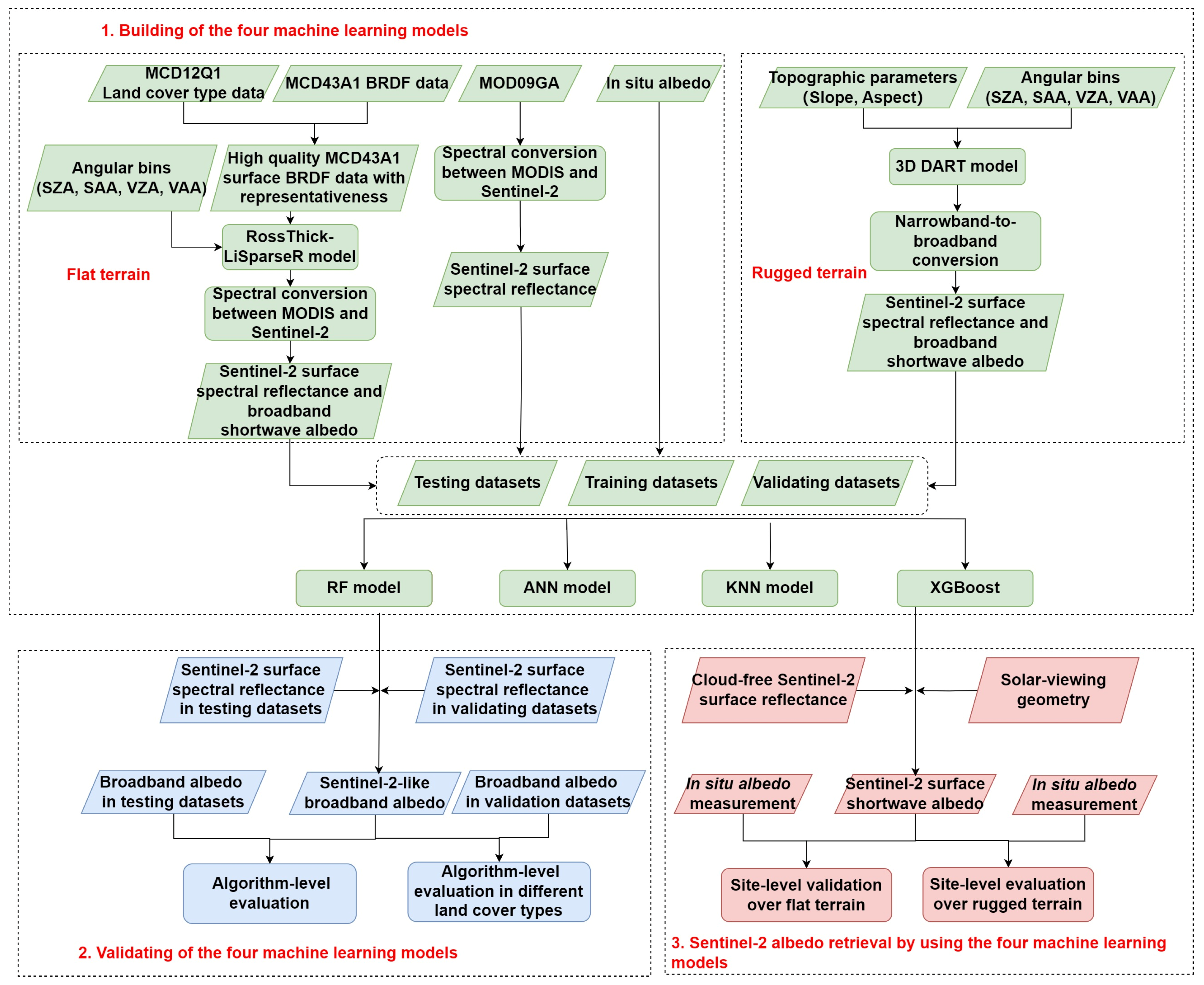
2.1. Data

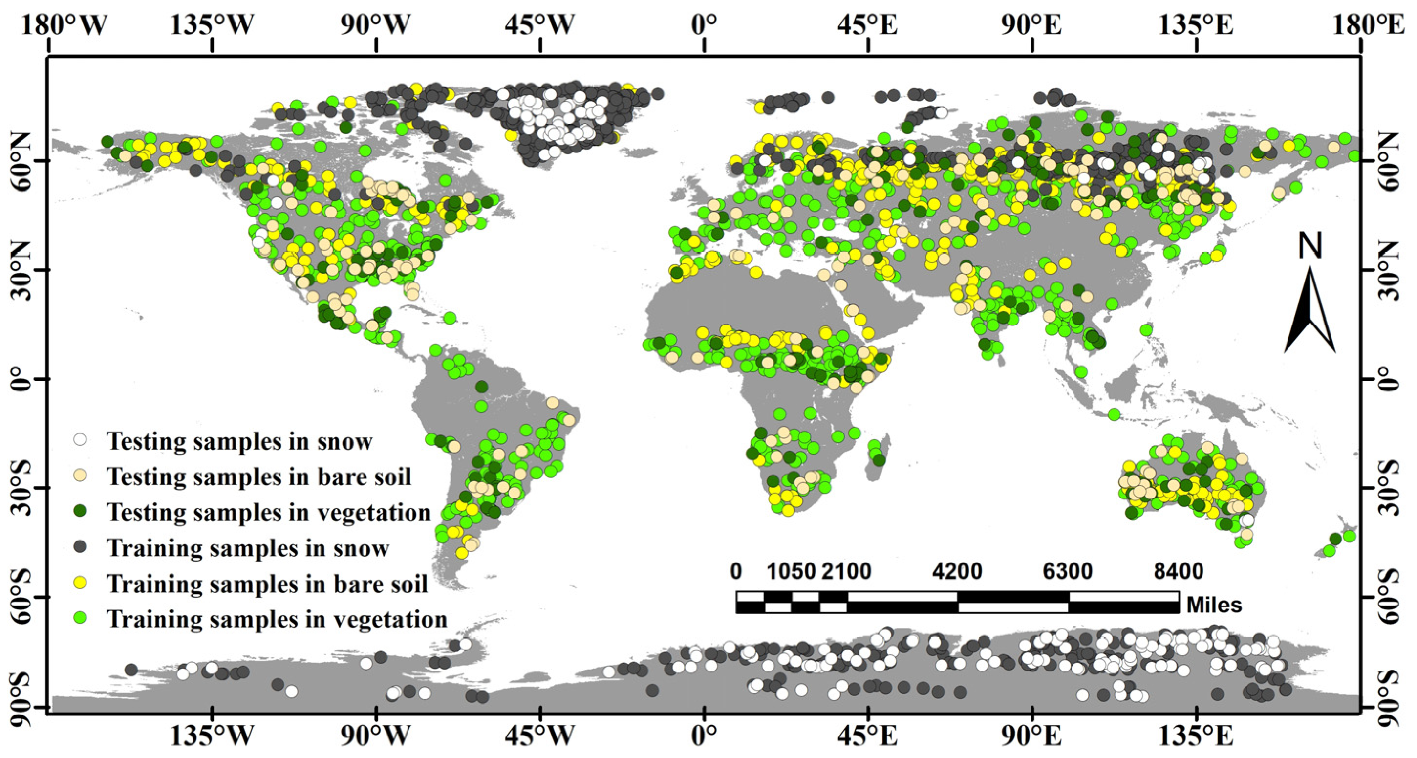
2.1.1. In Situ Observations

In situ surface albedo can be collected from the sites from radiation flux networks distributed worldwide, such as Fluxnet (which contains AmeriFlux, EuroFlux, AsiaFlux, and so on). In this study, in situ albedo measurements were mainly obtained from AmeriFlux and EuroFlux. AmeriFlux and EuroFlux are the core regionally distributed parts of Fluxnet [30]. AmeriFlux (http://ameriflux.lbl.gov/ (accessed on 20 April 2021)) was established in 1996 [31]. EuroFlux has been funded by the European Union since 1996 (http://www.europe-fluxdata.eu/ (accessed on 22 April 2021)).
In this study, 116 sites were from flat terrain, 20 sites were from rugged terrain, and 14 sites were from snow-covered areas (Table A1) (Figure 1). In situ albedos were calculated from the ratio of upward shortwave radiation to downward shortwave radiation at the local solar noon (e.g., from 11:00 to 13:00). In this paper, we used the measured values at the site to verify the satellite-retrieved albedo.

2.1.2. Sentinel-2 Data

The Sentinel-2 multispectral instrument (MSI) sensor provides multispectral data at a high resolution over the earth’s surface, with two satellites and a revisit time of 5 days [18]. Compared to previous satellites such as the Landsat series, Sentinel-2 has the advantage of a higher spatial resolution and a shorter revisit cycle [32]. The max viewing zenith angle (VZA) of Sentinel-2 is smaller than 20° [32].
In this study, we only used four 10 m visible and NIR bands (Table 1) in 2019. The surface reflectance and the observation geometry (including the solar zenith angle (SZA), solar azimuth angle (SAA), satellite viewing zenith angle (VZA), and satellite viewing azimuth angle (VAA)) of the Sentinel-2 satellite were calculated by using the SNAP software in the Python language. The 10 m land cover type datasets were downloaded from the ESA World Cover datasets [33].

2.1.3. MCD43A1 BRDF/Albedo Product

The high-quality 500 m Collection V061 daily MODIS BRDF products (MCD43A1) (https://urs.earthdata.nasa.gov/ (accessed on 4 May 2021)) were used to provide three kernel coefficients to drive the linear kernel-driven BRDF model (the Rossthick-LiSparseR model herein) for the simulation of narrowband surface reflection and broadband albedos [34]. Only the high-quality MCD43A1 data, marked with the quality flag of 0 in the MCD43A2 products, from the first seven bands were selected in this paper. To make the MCD43A1 data have representativeness, 1200 samples of MODIS BRDF data were selected from three land cover types including vegetation, soil, and snow (Figure 2), which were classified by using the same MODIS land cover products and the NDVI products as Lin et al. [27].

2.1.4. MOD09GA Product

The MOD09GA Version 6 product provides the surface spectral reflectance of the MODIS Terra satellite across the blue band to shortwave infrared bands using sinusoidal projection. In this study, seven bands of surface reflectance from the MOD09GA products were extracted from snow-covered stations to build a relationship with the site surface albedo.

2.2. Methods

The methodology in this paper was divided into three steps (Figure 3). First, the training and testing datasets for the four machine learning algorithms were generated based on two methods, including: (1) using the MCD43A1 BRDF products and the Rossthick-LiSparseR model to simulate narrowband surface and broadband albedo over the flat terrain; (2) using in situ observations and satellite-based surface reflectance at the snow-covered surface to refine the training datasets over the snow-covered surface; (3) using the DART model to simulate sloping surface reflectance and broadband albedo over the rugged terrain. Second, the training and testing datasets were used to drive the machine learning models and then to generate Sentinel-2 albedo. Third, the derived surface albedo was compared with in situ albedo observations to check the performance of these algorithms. Here, when the slope was greater than 5°, we used the rugged terrain models to retrieve the surface albedo of the Sentinel-2 image. In other cases, we used the flat terrain models to retrieve the surface albedo.

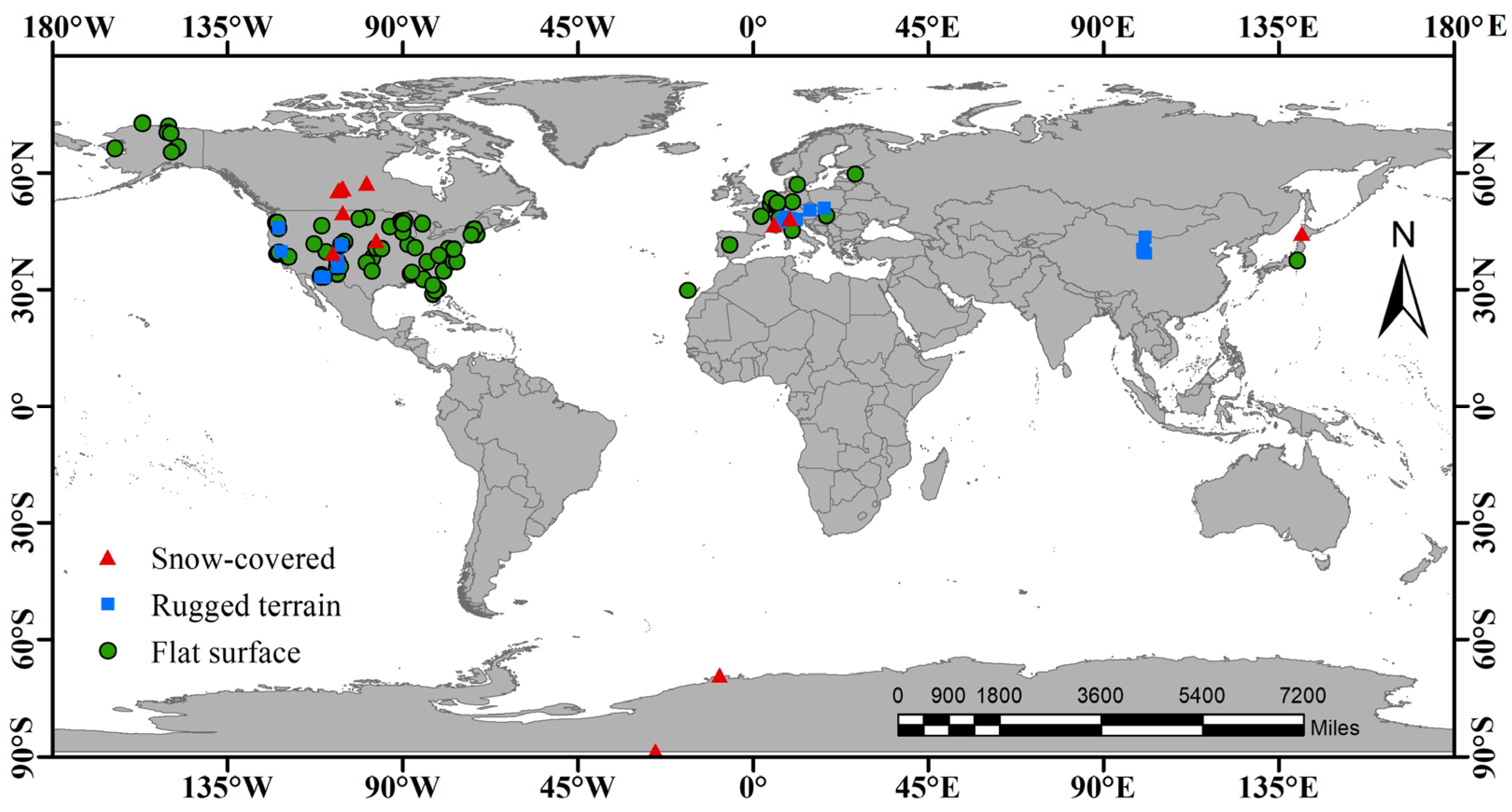
2.2.1. Training and Testing Dataset Simulation over Flat Terrain

Over flat terrain, the training and testing datasets were the first assurances to drive and validate the machine learning models. In this study, eight predictor variables were selected to produce the surface albedo (including BSA and WSA) from three main groups including narrowband spectral band reflectance at Sentinel-2 bands in 10 m, solar, and view observation geometries (i.e., SZA, VZA, and RAA), and land cover type. To produce the BSA, the local solar zenith angle (LSZA) was added apart from the former eight predictor variables.
The narrowband spectral surface reflectance and broadband albedos were simulated by using the MCD43A1 BRDF data and the RossThick-LiSparseR model [34]. Firstly, we used the MCD43A1 BRDF datasets, the MCD43A2 datasets, and the MCD12Q1 land cover type data to select the high-quality MCD43A1 BRDF datasets with representativeness generated by Qu et al. [35]. Then, we used the selected MCD43A1 data to simulate spectral surface reflectance and narrowband surface albedo across seven MODIS spectral bands using the RossThick-LiSparseR BRDF model [34,36,37,38]:
R θ s , θ v , ϕ , λ = f i s o θ s λ + f v o l λ k v o l θ s , θ v , ϕ + f g e o λ K g e o θ s , θ v , ϕ
α w s λ = f i s o λ k i s o λ + f v o l λ k v o l λ + f g e o λ k g e o λ
α b s θ s , λ = f i s o λ g 0 i s o + g 1 i s o θ s 2 + g 2 i s o θ s 3 + f v o l λ g 0 v o l + g 1 v o l θ s 2 + g 2 v o l θ s 3 + f g e o λ g 0 g e o + g 1 g e o θ s 2 + g 2 g e o θ s 3
The equation includes the following components: R ( θ s , θ v , ϕ , λ ) represents the surface reflectance under specific illumination and viewing conditions, with θ s representing the solar zenith angle, θ v representing the viewing zenith angle, ϕ representing the relative azimuth angle, and λ representing the wavelength of light. The components k g e o and k v o l denote the geometric optical and volumetric scattering kernels, which are characterized by functions of the illumination and viewing geometry. Additionally, f g e o and f v o l represent the weights assigned to these two kernel functions, while f i s o denotes the isotropic weight.
The seven simulated narrowband spectral surface reflectance bands were converted to four narrowband spectral surface reflectance bands of the Sentinel-2 by employing a model that utilizes band conversion coefficients. The band conversion coefficients were preferred to be built based on a linear regression approach from the MODIS satellite reflectance to Sentinel-2 reflectance (called Sentinel-2-like reflectance) coupled with the relative spectral response (RSR) function profiles of these two satellites and the high-quality ground-based spectra data, which were collected from Lin et al. [27], the China typical object spectral dataset [39], a quantitative remote sensing book [40], the Greenland spectral dataset [35], and the USGS digital spectral library [41]. Additionally, the broadband albedo was transferred from seven narrowband spectral albedos using the narrowband-to-broadband model by Liang et al. [42].
The simulated Sentinel-2 surface reflectance was generated by using the RTLSR model over a set of solar/view observation geometries (including SZA, VZA, and RAA). The SZA ranged from 0° to 80° with an interval of 4°, the VZA was in the range of 0°–12° with an interval of 6°, and the RAA was in the range of 0°–180° with an interval of 30°. The broadband albedo was simulated at the local solar zenith angle (LSZA), with the LSZA in the range of 0°–80° with an interval of 4°. Considering that both the surface reflectance and albedo were smaller than 1 and larger than 0, only the reasonable data were used to build the training, testing, and validating datasets. At the same time, we used in situ albedo recorded from 14 ground stations to refine the broadband albedo by directly using in situ albedo records to correct the broadband albedos, which were simulated by using the BRDF model in the training datasets. Generally, 80% of the surface reflectance simulations were used as training datasets and 20% of the simulations were used as testing datasets (Table 2).

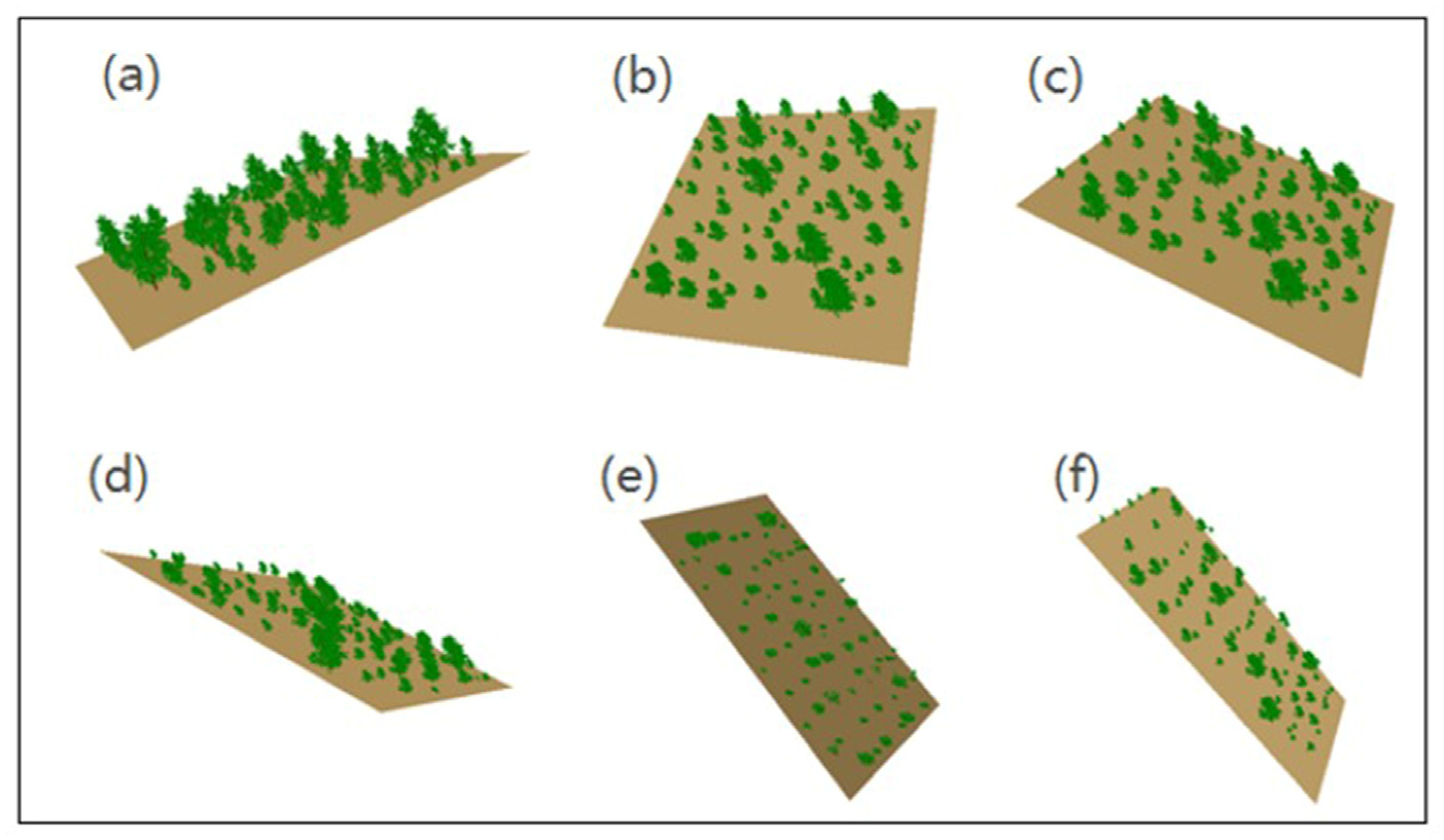
2.2.2. Training and Testing Datasets Simulation over Rugged Terrain

The discrete anisotropic radiation transfer model (DART) is a three-dimensional radiation transfer model based on an efficient Monte Carlo light transfer algorithm (i.e., bidirectional path tracking), which simulates the radiation transfer of electromagnetic wave radiation from visible light to thermal infrared bands in real three-dimensional structural scenes. With the DART model, we can build a complex mountain scene and obtain high-quality surface reflectance and surface albedo. Over rugged terrain, several sets of 100 m × 100 m scenes with a resolution of 10 m were created first. The configurations of canopy structures were produced in the scene, with the LAI varying from 1 to 7 at an interval of 2; the solar zenith angle ranged from 0° to 60°, divided by 10° intervals; the viewing zenith angle varied from 0° to 30°, divided by 10° intervals; and the relative azimuth varied from 0° to 180°, divided by 45° intervals. The topographic parameters of the scenes were also considered, with the slope varying from 0° to 60° at intervals of 10°, and the aspect varied from 0° to 180° at intervals of 45°. Finally, we obtained a total of 4900 forest scenes (Figure 4). Over these scenarios, the narrowband surface reflectance broadband albedos were simulated by using the DART model. The slope, aspect, SZA, VZA, RAA, and four-band reflectance (Blue, Green, Red, and NIR) were input variables, and the BSA and WSA were target variables to train and test them with machine learning models. Detailed information of the training datasets and testing datasets is shown in Table 3.

2.2.3. Machine Learning Models

Machine learning models have been widely used in the remote sensing field. Machine learning models, such as random forest (RF) and artificial neural networks (ANN), can analyze and process large amounts of training datasets to obtain more accurate prediction results. This study utilized four machine learning models to generate land surface albedo products, including the RF, ANN, k-nearest neighbor (KNN), and XGBoost (XGBT) models. The RF model is a nonlinear model. Its principle is to build forests by creating decision trees, which can be applied to classification and regression problems [29,43,44]. It uses input data to build a large number of trees for prediction [45]. RF model has two key parameters: one is the number of decision trees (Ntree), and the other is the number of selected variables [46]. The RF model builds multiple decision trees and combines their outputs to make a final prediction. Additionally, it is robust to overfitting and can handle missing data without the need for data preprocessing. RF can also handle a large number of features and can be used for feature selection. Artificial neural networks (ANNs) can establish the nonlinear complex relationship between explanatory variables and dependent variables, and efficiently solve complex problems [47]. ANN models are nonparametric; input information is obtained from the input layer, then transferred to the middle layer, and then transferred to the output layer through the weighting process of each middle layer and activated by the excitation function, and finally output from the output layer They are more acceptable than statistical remote sensing methods [48]. ANN models can handle nonlinear relationships between inputs and outputs, and can be used for both classification and regression. They can learn from large amounts of data and can generalize well to new data. Additionally, they are robust to noisy or incomplete data and can be used for image and speech recognition. K-nearest neighbor (KNN) is one of the simplest machine learning algorithms, which does not learn from the training dataset immediately; instead, it stores the dataset and at the time of application, it performs an action on the dataset. It provides a robust approach to produce spatially contiguous predictions of attributes and is widely applied in remote sensing science [49]. KNN does not make any assumptions about the underlying distribution of the data and can adapt to any type of data, which make it easy to implement and interpret. The XGBT algorithm is an enhanced and optimized version of GBDT, which is developed from the GBDT algorithm. XGBT can be seen as an additive model. It can effectively solve the problems of regression and classification by predicting the results through accumulation [50]. XGBT can handle a large number of features and provides feature importance scores, which can be used for feature selection. Additionally, it is fast and can handle large datasets. We used the training datasets to drive the machine learning models. To determine the optimal metaparameters for all four machine learning models, we employed 10-fold cross-validation. We used Python to complete all the construction and verification of the machine learning models.

2.2.4. Sentinel-2 Albedo Retrieval by Using Machine Learning Models

The first step was to download cloud-free Sentinel-2 surface reflectance data using the Google Earth Engine (GEE). Next, we utilized the cloud probability product of Sentinel-2 to eliminate pixels that were affected by cloud cover or shadows. Additionally, we manually rechecked the surface reflectance to make sure that there were not any cloud-covered pixels over the Sentinel-2 surface reflectance. Meanwhile, we also obtained the solar–viewing geometry, including the SZA, VZA, RAA, and LSZA, from the auxiliary files. We used the surface reflectance, the solar–viewing geometry, and the land cover types as inputs for driving the machine learning models to predict the BSA and WSA.

2.2.5. Machine Learning Models’ Performance Evaluation

Three commonly used metrics, including bias, root mean square error (RMSE), and coefficient of determination (R2), were used for accuracy assessments. We assessed the accuracy of the machine learning models in two levels: algorithm-level evaluation and site-level evaluation.
B i a s = A l b e d o p A l b e d o t
R 2 = i = 1 n A l b e d o p i A l b e d o p i A l b e d o t i A l b e d o t i i = 1 n A l b e d o p i A l b e d o p i 2 i = 1 n A l b e d o t i A l b e d o t i
R M S E = i = 1 n A l b e d o p i A l b e d o t i 2 n
The equation includes the following components: A l b e d o p is the albedo value predicted by the model, A l b e d o t is the albedo value used for verification, and n is the number of albedo values.
We used the training dataset and testing dataset to validate the machine learning models and evaluate their accuracy. The broadband albedos of the training and testing datasets were used here as the reference dataset to assess the accuracy of the machine learning models. We first applied the four models to the land surface reflectance, the SZA, the VZA, and the RAA in the training and testing datasets to generate the broadband BSA and WSA (called the predicted BSA and WSA), respectively. We then further directly compared the model-derived albedo with the simulated broadband albedo in the training datasets and testing datasets. In particular, the overall accuracies of the machine learning models were assessed by using the testing datasets.
We also used the in situ observations to show the performance of the models to generate Sentinel-2 albedos. We used the measured albedo of the site to validate the machine learning model’s inversion of the Sentinel-2 albedo. Considering the effects of diffuse radiation, we transferred the Sentinel-2 BSA and WSA to blue-sky albedo (hereafter called albedo) by coupling with the sky diffuse ratio [26].

3. Results

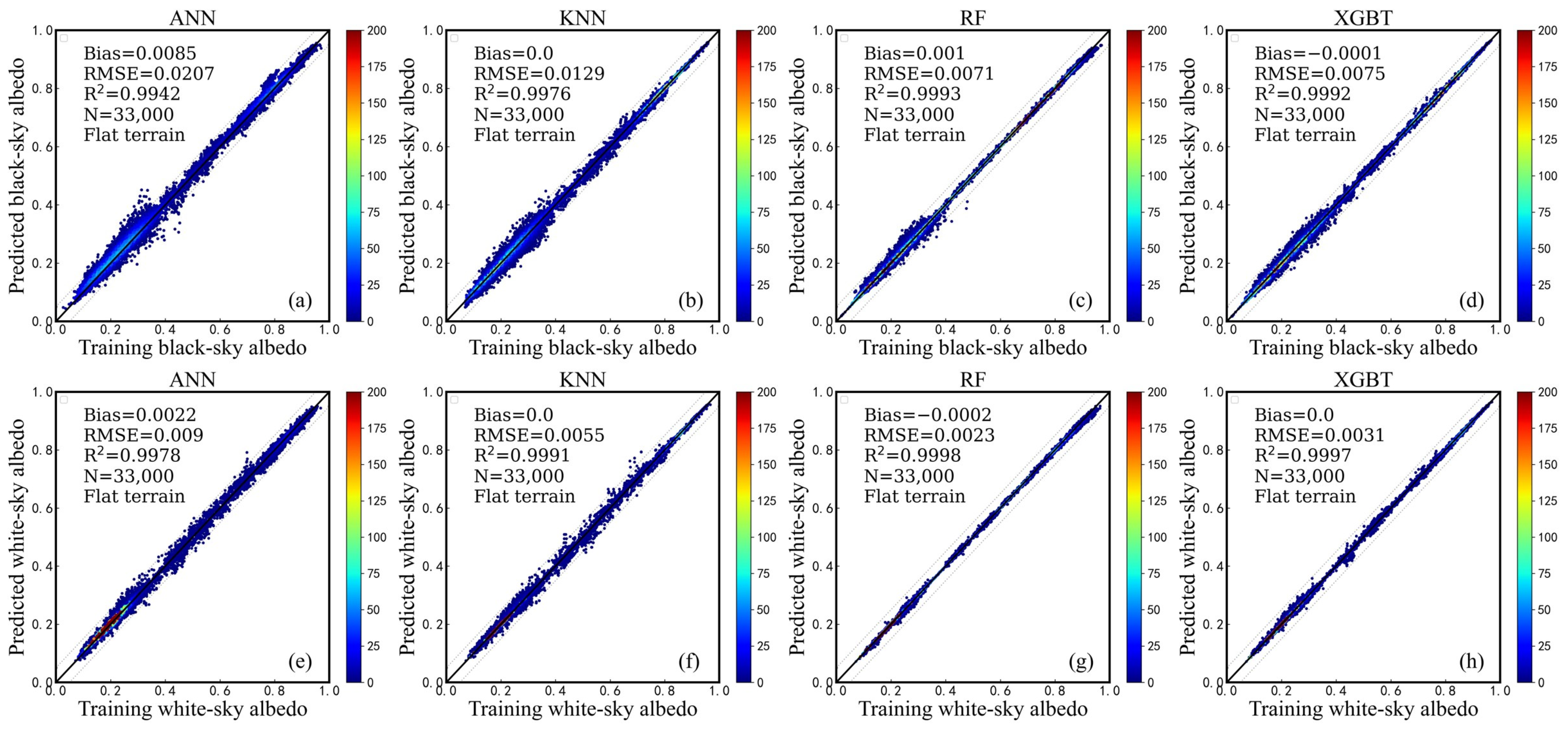
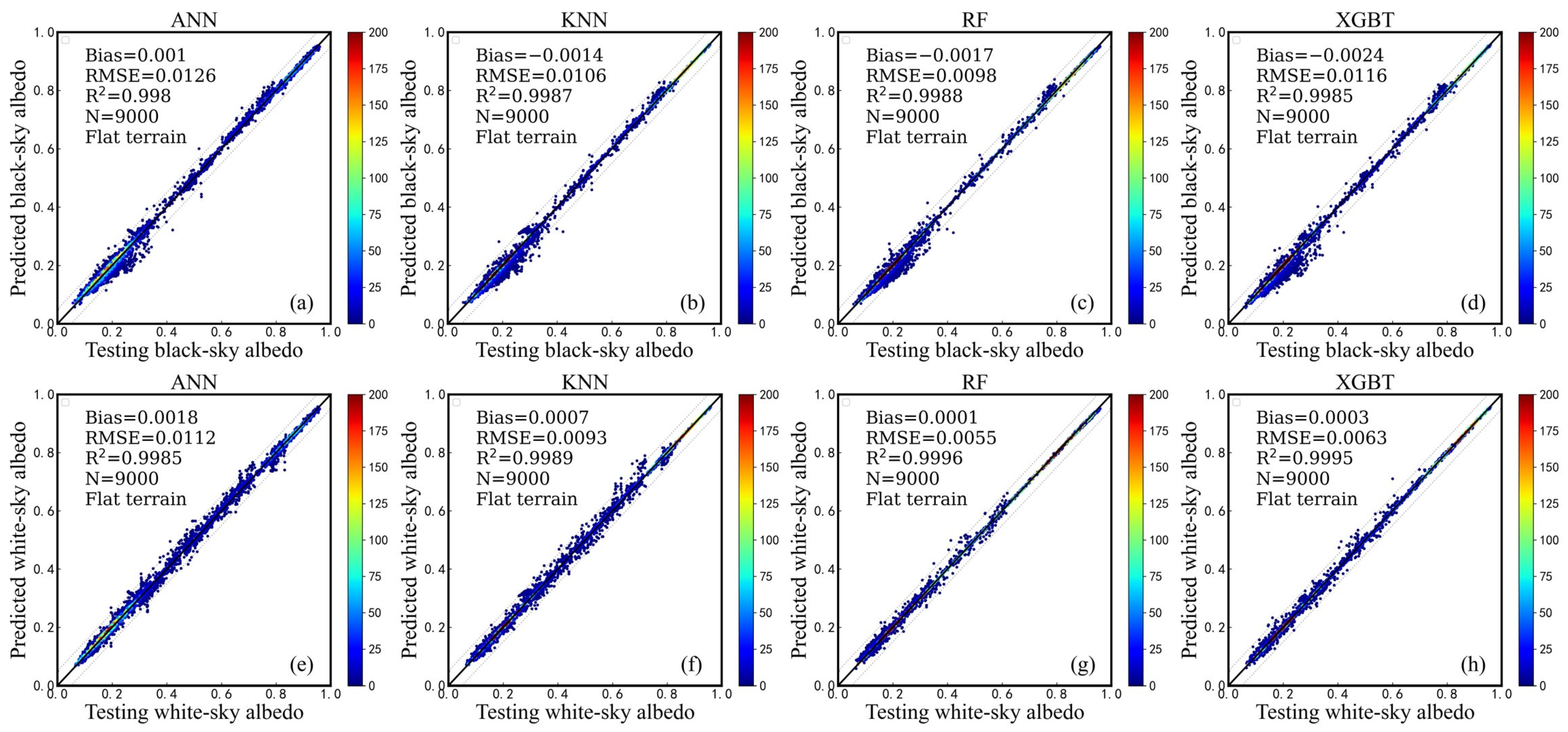
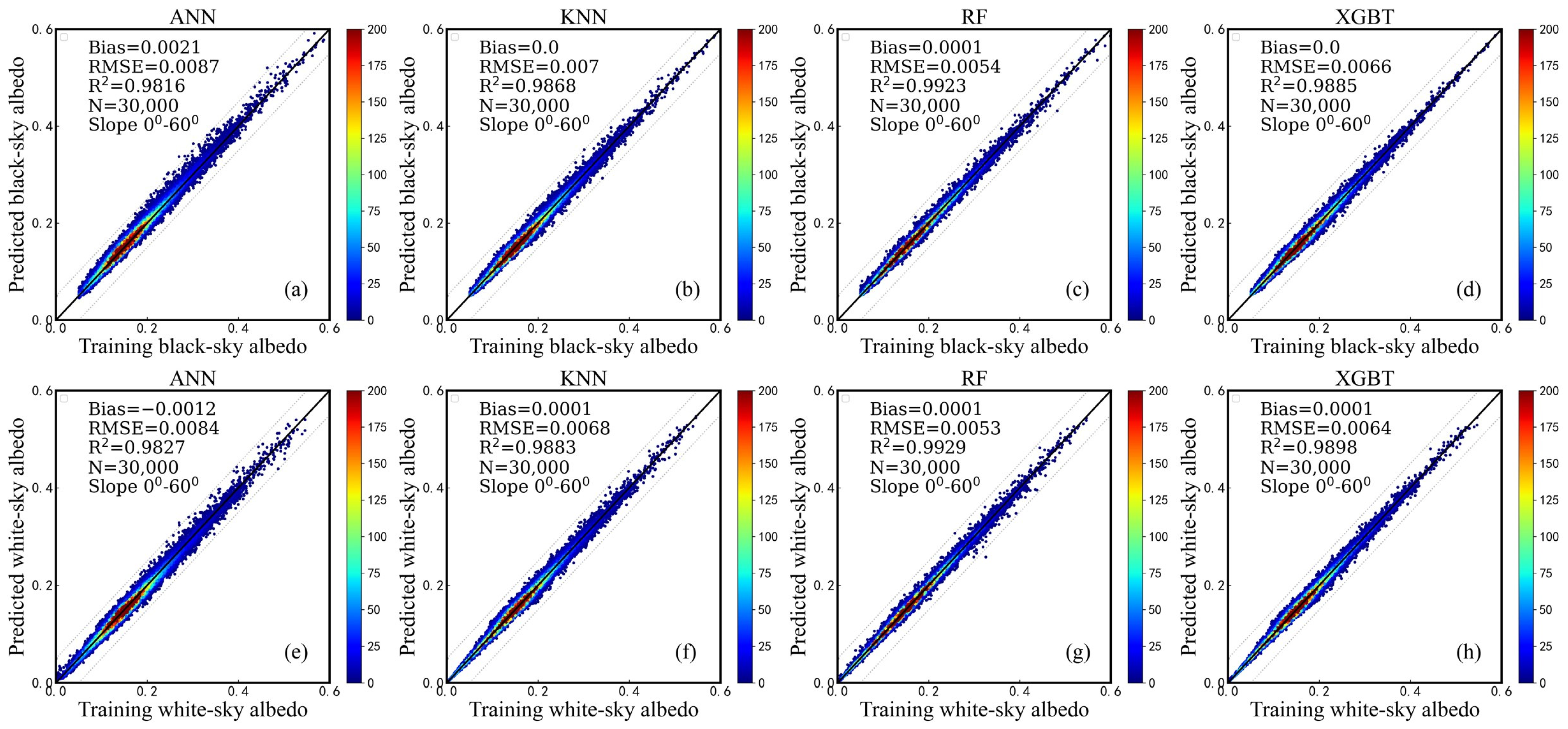
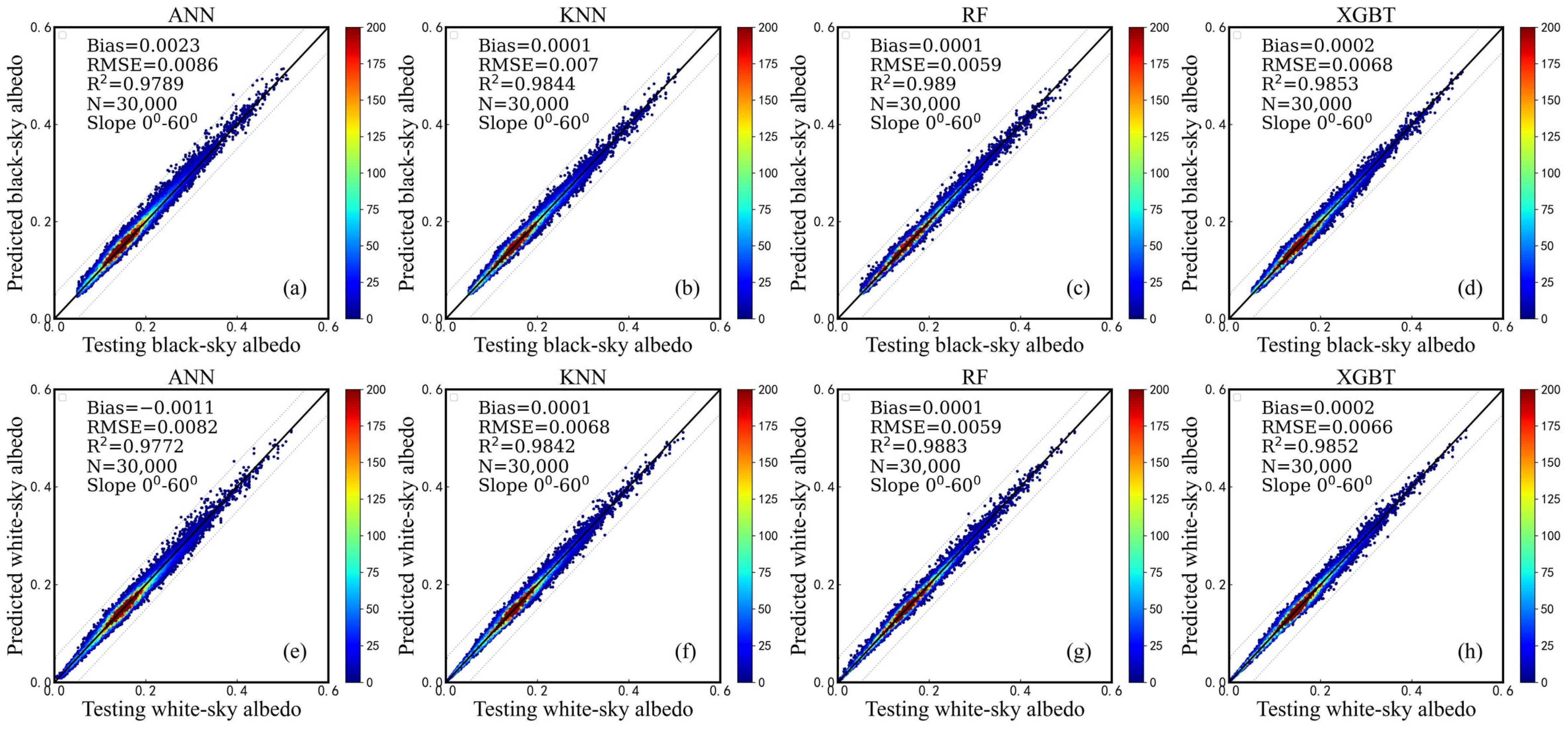
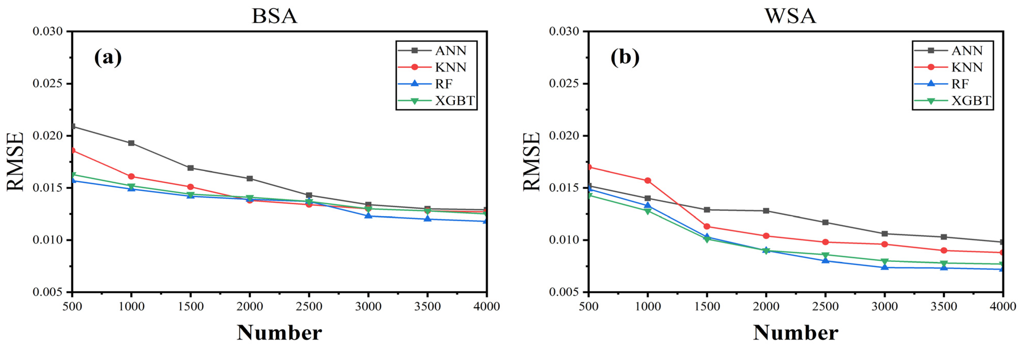
3.1. The Performance of the Machine Learning Model

Figure 5a–d show the training accuracy of estimating the BSA by using the machine learning models (ANN, KNN, RF, and XGBT). Overall, the predicted BSA generated by the machine learning models had better agreement with the BSA in the training datasets (called the training BSA hereafter). The RF model showed better performance than the other machine learning models during the training of the BSA, with a bias of 0.001, RMSE of 0.0071, and R2 of 0.9993. The predicted BSA generated by the XGBT model showed a slightly larger uncertainty than that generated by the RF model and a smaller uncertainty than that generated by the ANN model and KNN model, with a bias of −0.0001, RMSE of 0.0075, and R2 of 0.9992. The predicted BSA generated by using the KNN model also had good agreement with the training BSA, with a bias of 0.0, RMSE of 0.0129, and R2 of 0.9976. The predicted BSA generated by using ANN model had the largest uncertainty compared to that generated by using the other three machine learning models, with a bias larger than 0.0085, RMSE larger than 0.0207, and R2 larger than 0.9942.
Figure 5e–h show the accuracy of estimating the WSA generated by using the machine learning models (ANN, KNN, RF, and XGBT) for the training datasets. Generally, all of the four machine learning models showed better performances in retrieving the WSA than in the retrieval of the BSA, which is illustrated by the smaller RMSE of the predicted WSA than the BSA. Similarly, the predicted WSA generated by using the ANN model showed larger uncertainty than that generated by the other three machine learning models, with a bias of 0.0022, RMSE of 0.009, and R2 of 0.9978. The predicted BSA generated by the KNN model also showed slightly larger uncertainty than that generated by using the RF model and XGBT model, with a bias of 0.0, RMSE of 0.0055, and R2 of 0.9991. The RF model and the XGBT model had similar performance, with a Bias of −0.0002 and 0.0, RMSE of 0.0023 and 0.0031, and R2 of 0.9998 and 0.9997, respectively.
Figure 6a–d show the accuracy of the predicted BSA when using the machine learning models (ANN, KNN, RF, and XGBT) and the testing datasets. The results show that the predicted BSAs generated by the four machine learning models matched well with the BSA in the testing datasets, with low biases and uncertainty and high R2 values. Generally, the bias varied from −0.0024 to 0.001, the RMSE ranged from 0.0098 to 0.0126, and the R2 values were all equal to 0.99. The RF model performed better than the ANN, KNN, and XGBT models, with an RMSE smaller than 0.0098. The KNN model showed slightly less confidence than the RF model, with an RMSE of 0.0106 but a larger bias than that of the RF model, at −0.0014. Larger uncertainty between the predicted BSA and testing BSA occurred in the application of the ANN model, with an RMSE larger than 0.001 (Figure 6). The predicted WSA also matched well with the WSA in the testing datasets, with the bias varying from 0.0001 to 0.0007, the RMSE varying from 0.0055 to 0.0112, and the R2 being larger than 0.9985, respectively (Figure 6e–h).
Figure 7a–d show the training accuracy of estimating the BSA when using machine learning models (ANN, KNN, RF, and XGBT) over rugged terrain. Similarly to that over flat terrain, the RF model showed better performance than the other machine learning models during the training of the BSA, with a bias of 0.0064, RMSE of 0.0064, and R2 of 0.9923. The predicted BSA generated by the XGBT model showed a slightly larger uncertainty than that generated by the RF model, with a bias of 0.0001, RMSE of 0.0076, and R2 of 0.9885. The predicted BSA generated by using the KNN and ANN models showed a larger uncertainty than the other two models, with a bias of 0.0001, RMSE of 0.0008, and R2 of 0.9868 for the KNN model, and a bias larger than 0.0022, an RMSE larger than 0.0097, and an R2 larger than 0.9816 for the ANN model.
Figure 8e–h show the training accuracy of the machine learning models (ANN, KNN, RF, and XGBT) for the generation of the Sentinel-2 WSA over rugged terrain. The predicted WSA generated by using the ANN model also showed larger uncertainty than that generated by the other three machine learning models, with a bias of −0.0012, RMSE of 0.0094, and R2 of 0.9827. The predicted BSA generated by the KNN model showed a slightly larger uncertainty than that generated by using the RF model and XGBT model, with a bias of 0.0001, RMSE of 0.0078, and R2 of 9883. The RF model and the XGBT model had similar performance, with a bias of 0.0001, RMSE values of 0.0063 and 0.0074, and R2 values of 0.9929 and 0.9898, respectively.
Figure 8a–d show the accuracy of the predicted BSA when using the machine learning models (ANN, KNN, RF, and XGBT) for the testing datasets over rugged terrain. The results show that the predicted BSAs generated by the four machine learning models matched well with the BSA in the testing datasets, with low biases and uncertainty and high R2 values. Generally, the bias varied from 0.0001 to 0.0023, the RMSE ranged from 0.0069 to 0.0096, and the R2 values were both equal to 0.978. The RF model performed better than the ANN, KNN, and XGBT models, with an RMSE smaller than 0.0069. The largest uncertainty between the predicted BSA and testing BSA occurred in the application of the ANN model, with an RMSE larger than 0.0096. The predicted WSA also matched well with the WSA in the testing datasets over rugged terrain, with the bias varying from −0.0011 to 0.0002, the RMSE varying from 0.0069 to 0.0092, and the R2 being larger than 0.9772 (Figure 8e–h).

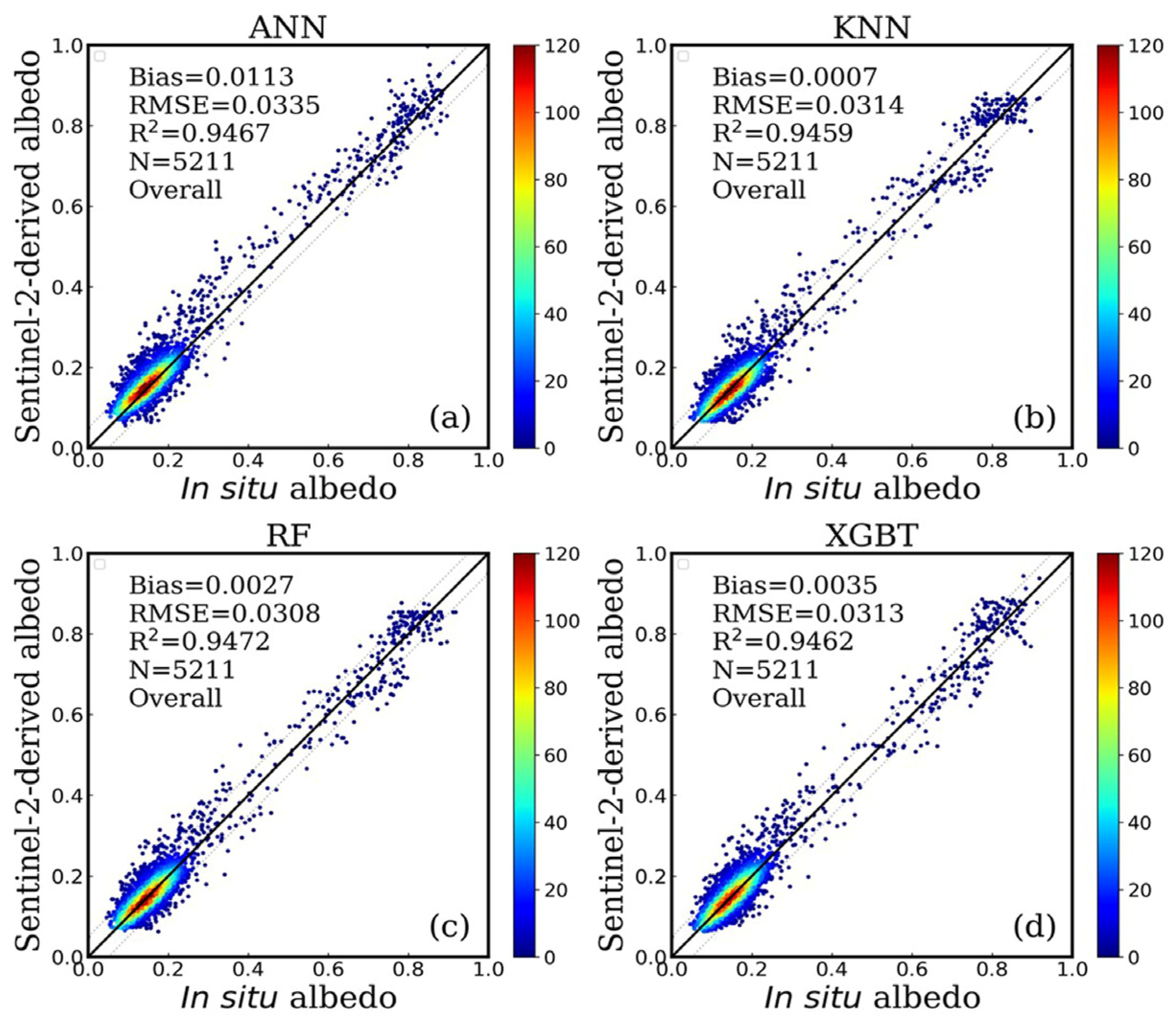
3.2. Site-Level Comparison of the Sentinel-2 Albedos over Flat Terrain

The Sentinel-2 BSA and WSA were coupled to calculate the Sentinel-2 blue-sky albedo. The performances of these machine learning models were assessed by comparing the Sentinel-2 blue-sky albedo with in situ albedo measurements in the spatial response range of tower-based albedo observation. The results show that the Sentinel-2-based albedo generated by using the four machine learning models matched well with the in situ observations, with low biases, low uncertainty, and high R2 values (Figure 9). Generally, the ANN model had a worse performance than the other three models, with a bias of 0.0113, RMSE of 0.0335, and R2 of 0.9467. The Sentinel-2 albedo generated by using the KNN model had a bias of 0.0007, RMSE of 0.0314, and R2 value of 0.9459. The RF-model-derived Sentinel-2 albedo had great agreement with the in situ albedo, with a bias of 0.0027, RMSE of 0.0308, and R2 value of 0.9472. The XGBT-model-generated albedo had a bias of 0.0035, RMSE of 0.0313, and R2 value of 0.9462 when compared with the in situ albedo (Figure 9). Similarly to the results of the training and testing datasets, the RF model showed the best performance compared to the other three machine learning models to retrieve Sentinel-2 albedo, which is demonstrated by the smallest RMSE shown in Figure 9. Additionally, the ANN showed the worst performance compared to the other three models.
For snow-covered surfaces (Figure 10), the accuracies of the models (ANN, KNN, RF, and XGBT) were lower than those for snow-free surfaces. The RF-model-derived albedo had a higher accuracy than that of the other three models, with a bias of 0.0031, RMSE of 0.0517, and R2 values of 0.8538; the accuracy of the XGBT-model-derived Sentinel-2 albedo was slightly lower than that generated by using the RF model, with a bias of 0.0014, RMSE of 0.0534, and high R2 values (0.8528); the accuracy of the KNN model was slightly lower than the RF and XGBT models, with a bias of 0.0086, RMSE of 0.0545, and R2 values of 0.8407; and the accuracy of the ANN-model-derived Sentinel-2 albedo was slightly lower than that of the other models, with a bias of 0.0276, an RMSE of 0.055, and a high R2 of 0.8655.

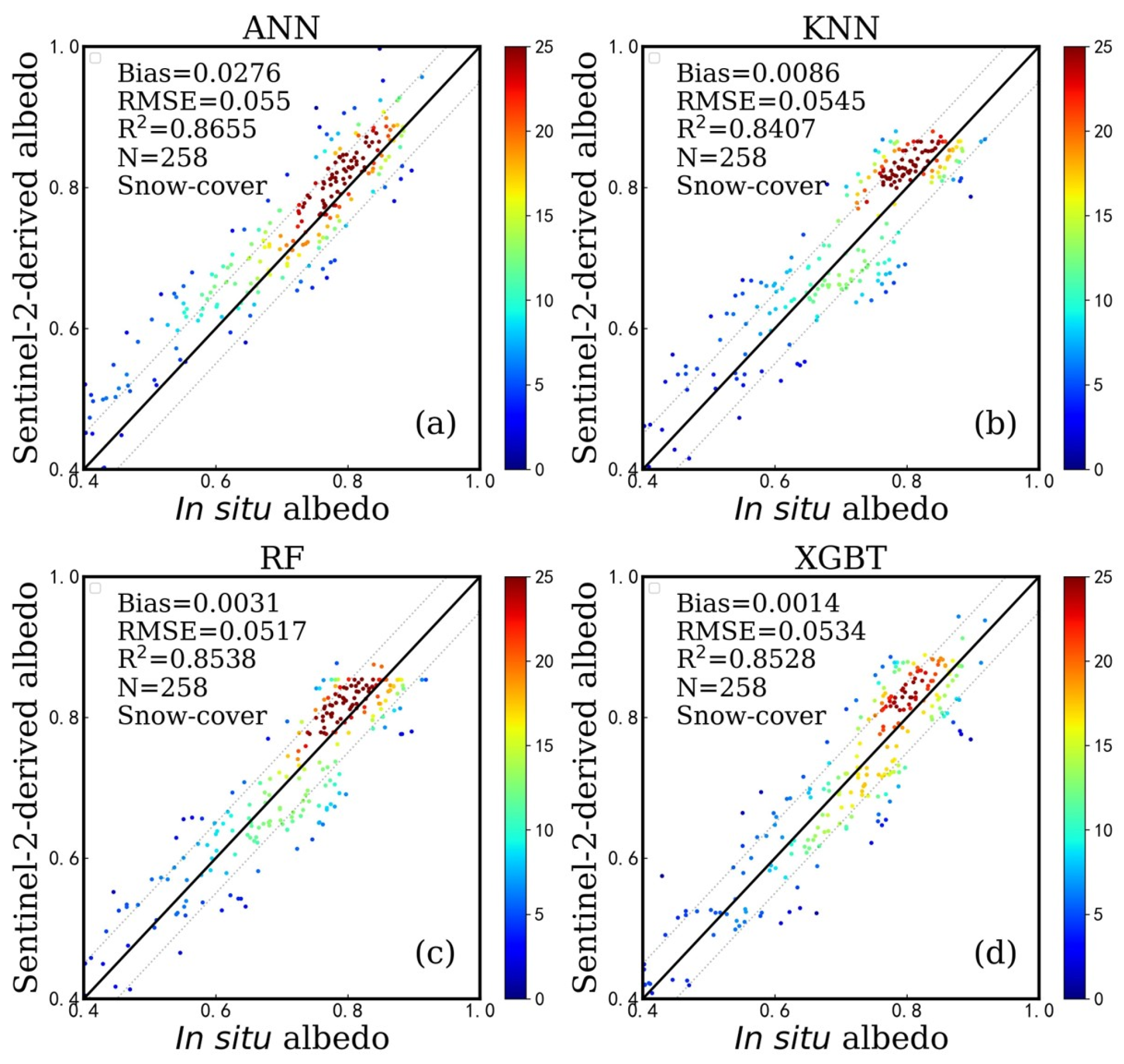
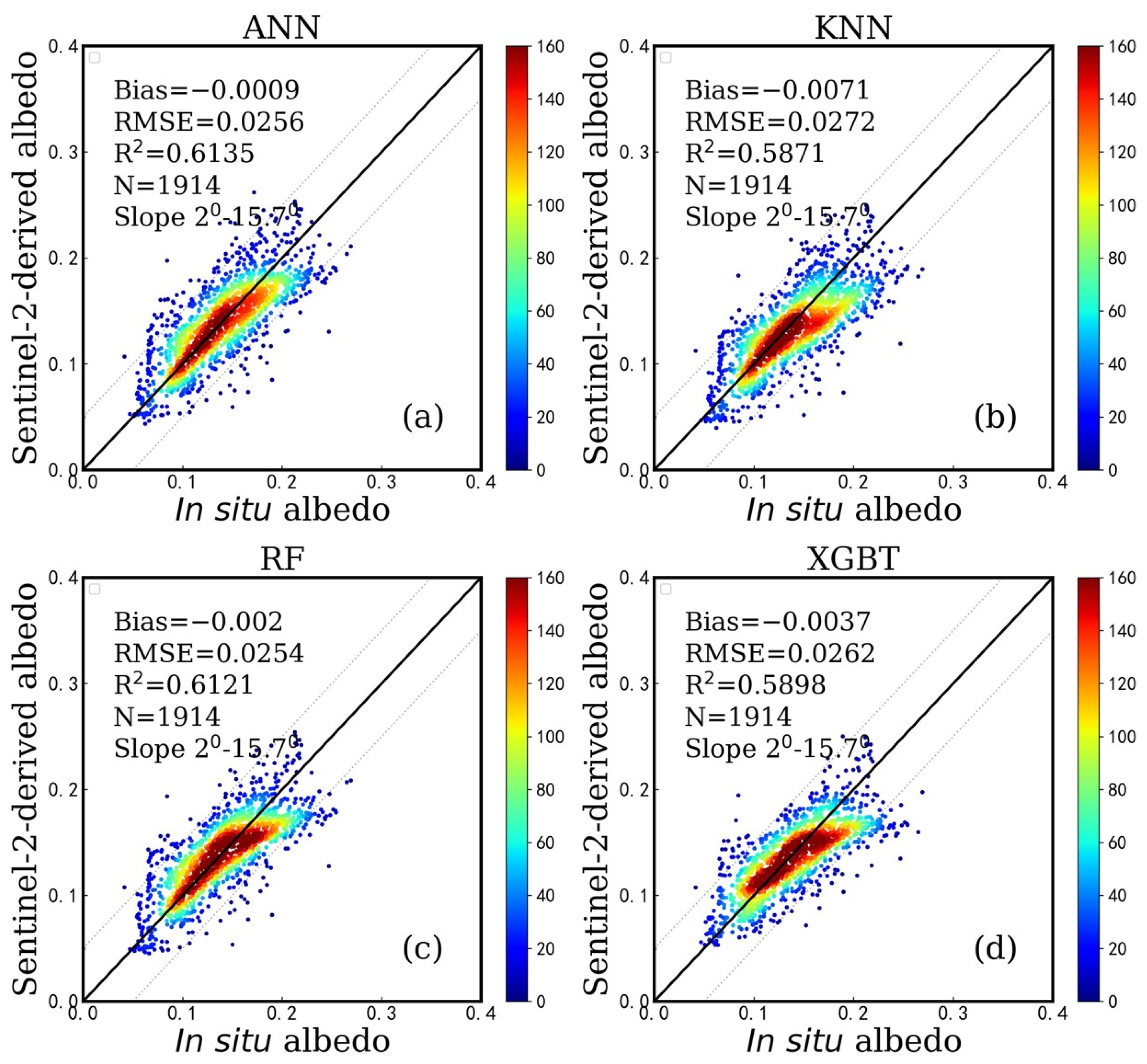
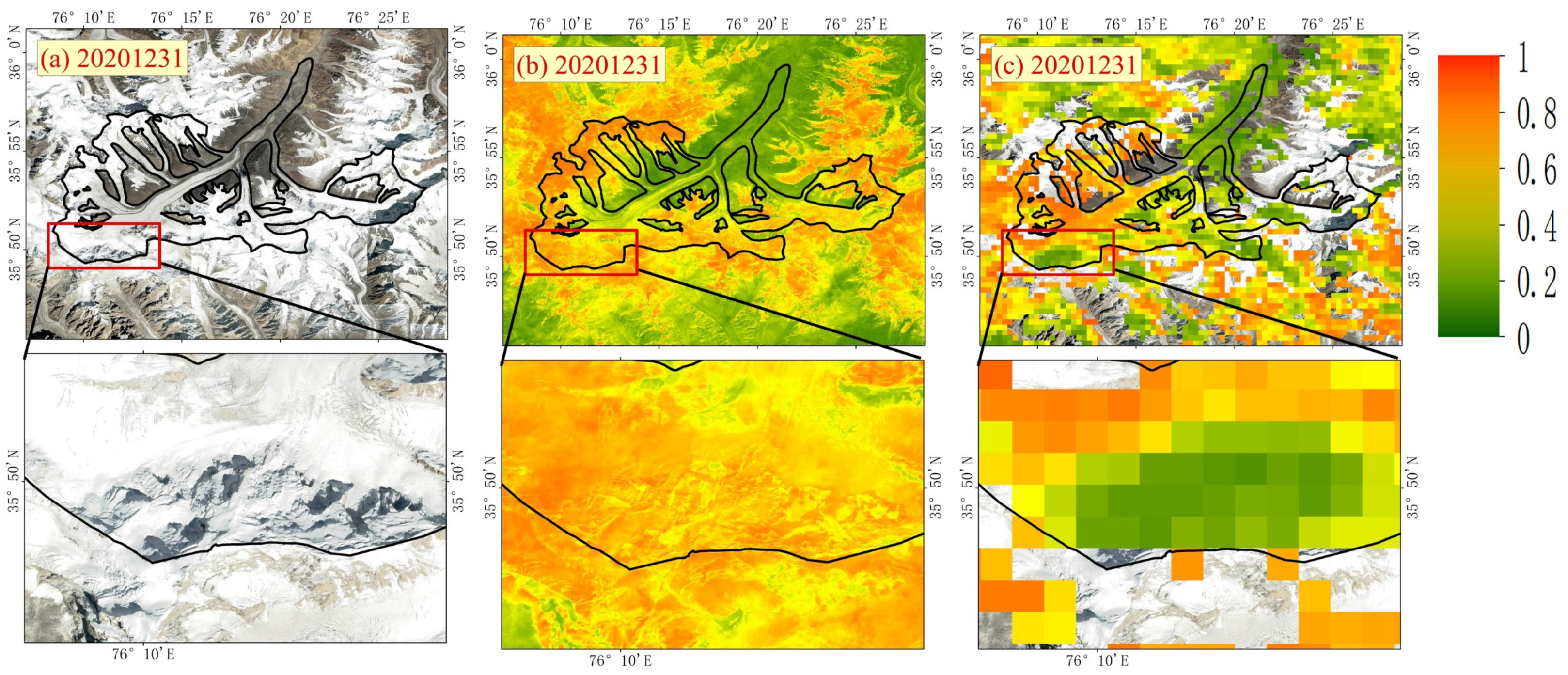
3.3. Site-Level Comparison of the Sentinel-2 Albedos over Rugged Terrain

The results show that the Sentinel-2-based albedo generated by using the four machine learning models matched well with the in situ observations over rugged terrain (Figure 11). Generally, the KNN model had worse performance than the other three models, with a bias of −0.0071, RMSE of 0.0272, and R2 of 0.5871. The Sentinel-2 albedo generated by using the ANN model had a bias of −0.0009, RMSE of 0.0256, and R2 value of 0.6135. The RF-model-derived Sentinel-2 albedo had great agreement with the in situ albedo, with a bias of −0.002, RMSE of 0.0254, and R2 value of 0.6121. The XGBT-model-generated albedo had a bias of −0.0037, RMSE of 0.0262, and R2 value of 0.5898 when compared with the in situ albedo (Figure 11).
We also assessed the performance of the Sentinel-2 albedo over surfaces with different topographic slopes (Table 4). In general, the machine learning methods were very effective in retrieving the surface albedo over rugged terrain. With the increase in slope angle, the uncertainty of the Sentinel-2 albedo increased. On the surface with the slope increasing from 0° to 5°, the RF-model-derived Sentinel-2 albedo showed great agreement with the in situ albedo, with a bias of −0.0023, RMSE of 0.0229, and R2 of 0.6367. The ANN-, KNN-, and XGBT-model-derived Sentinel-2 albedo showed similar accuracy, with biases of 0.0003, −0.0062, and −0.0041; RMSE values of 0.0239, 0.0251, and 0.0247; and R2 values of 0.6204, 0.5938, and 0.5832 for the ANN, KNN, and XGBT models, respectively. When the slope varied from 5° to 10°, the ANN-model-derived Sentinel-2 albedo also showed increased uncertainty, with a bias of −0.0049, RMSE of 0.0243, and R2 of 0.7223. The RF- and XGBT-model-derived Sentinel-2 albedo showed similar accuracy, with biases of −0.0053 and −0.0061, RMSE values of 0.0252 and 0.0257, and R2 values of 0.7035 and 0.6950, respectively. The KNN model showed worse performance than the other three models, with a bias of −0.0114, RMSE of 0.0277, and R2 of 0.6896. When the slope increased to larger than 10°, the accuracy of the XGBT-model-derived albedo was slightly lower than that of the other models, with a bias of 0.0051, RMSE of 0.0297, and R2 values of 0.4044. The ANN-, KNN-, and RF-model-derived Sentinel-2 showed similar accuracy, with biases of 0.0053, 0.0015, and 0.0093; RMSE values of 0.0309, 0.0302, and 0.0306; and R2 values of 0.3897, 0.4073, and 0.4088, respectively.

4. Discussion

An accurate estimation of land surface albedo at 10 m is essential for its application over a regional scale, especially for a deep understanding of the variation in land surface albedo in the climate change process at a fine spatial scale. Machine learning models provide a robust way to map surface albedo at a finer spatial scale of 10 m, which does not entail a complex process (such as the suitability of the BRDF model in such a fine spatial scale of 10 m and atmospheric effects) in land surface albedo retrieval. Here, we made a comparison to assess the performance of four popular machine learning models to generate Sentinel-2 albedos. We compared the error source of the machine learning models and the accuracy of the machine learning models.

4.1. The Performance of High-Resolution Surface Albedo over Snow/Ice-Covered Surfaces

In Figure 12, we compare the performance of the Sentinel-2 surface albedo and MODIS surface albedo in detecting the snow/ice-covered surfaces of the Insukati glaciers over the Qinghai–Tibet Plateau. We can clearly see that the retrieved Sentinel-2 albedo fits well with the distribution of snow/ice, which is shown by the large albedo over the heavy-snow-covered surface and the smaller albedo value over the snow-free surface (Figure 12b). The Sentinel-2 albedo could also effectively describe the trajectory of the valley glaciers, understand their actual range, and accurately reflect glacier changes with high precision (Figure 12b). The MODIS albedo only roughly reflected the ground truth features of glaciers and valleys and was unable to accurately reflect small differences in ground features (Figure 12c). Additionally, the Sentinel-2 albedo could also effectively represent the true surface albedo on the shaded side of mountainous terrain. Taking into account the impact of the terrain, the surface albedo was high on the sun-facing side and low on the shaded side.
However, the accuracy of machine learning models on ice and snow surfaces still needs to be improved (Figure 10). The Theia snow collection and snow detection are more accurate than the Sen2Cor outputs (ESA level 2 product) [51]. Lidar can effectively detect snow under a canopy and has high accuracy on complex terrains [52]. The operational high-resolution snow and ice monitoring (HRSI) algorithm yielded similar performances to the computationally intensive spectral unmixing approach, while retrieving the subcanopy ground fractional snow cover [53,54]. These outperforming tools give the chance to detect snow-covered surfaces and help us to improve the accuracy of albedo retrieval algorithms over snow-covered surfaces in the future.

4.2. Sensitivity Analysis of the Machine Learning Models

The quality and the quantity of the training datasets had the largest influence on the performance of the machine learning models. The quality of the training datasets was proved by the high suitability to regress the relationship between the narrowband surface reflectance and the broadband albedo, which was analyzed by Lin et al. [27]. To assess the sensitivities of the samples to drive the machine learning model, we assessed the sensitivity of the magnitude of the samples by adding the sample datasets during the training of the machine learning models with the gradient of 500 samples. We randomly selected 200 samples to test the performance of different machine learning models. Figure 13 shows the RMSEs between the predicted albedo, which were retrieved by using the machine learning models, and the testing albedo. We can see that with the increase in the quantity of samples, the RMSE decreased. Generally, the ANN is most sensitive to the quantity of samples for the generation of the BSA and WSA, followed by KNN, RF, and XGBT. In the generation of the WSA, the KNN is most sensitive to the quantity of samples, especially when the quantity of samples is smaller than 1500. When the number of samples reaches about 3000, the influence of the samples tends to be stable.

4.3. The Differences and Shortcomings of the Machine Learning Models

The machine learning models (ANN, KNN, RF, and XGBT) had better performance to retrieve Sentinel-2 albedo at 10 m. RF was the best, followed by XGBT and KNN, and ANN was the worst. The reasons for this are as follows:
In terms of algorithm principles: ANN simulates the process of mutual connection between neurons to achieve learning and prediction. The KNN algorithm classifies data based on its nearest neighbors. RF is composed of multiple decision trees. XGBT is a gradient boosting tree algorithm. In terms of suitable scenarios: ANN is suitable for complex classification and prediction problems with large amounts of data. KNN is suitable for clear feature classification problems. RF is suitable for classification and regression problems in large-scale datasets. XGBT is suitable for datasets with many features. In terms of computing performance: ANN requires iterative training through a backpropagation algorithm, which takes a long time. KNN has a short calculation time but requires large storage space. RF can perform parallel computing to improve computational efficiency. XGBT can efficiently handle large-scale datasets. Overall, the RF model outperformed the four machine learning models because it can effectively train large datasets and has a good antinoise ability to avoid overfitting issues. KNN has the problem of sample imbalance, which may lead to poor results [55]. ANN may become trapped in a local minimum on large datasets [56]. XGBT is suitable for processing structured feature data and unstructured data, which is not a good processing ability for unstructured data [57]. However, machine learning models are black box models. We can use them to generate Sentinel-2 albedo, but we cannot explain the mechanism of these models. The SHAP (SHapley Additive exPlanations) [58] method or other alternative methods paved the way to explaining the essential output parameters of the model, which may have been used in this work to help us understand the mechanism of machine learning models.

5. Conclusions

Data-driven machine learning algorithms demonstrate better performance in dealing with probable nonlinear regression progress for remote sensing data retrieval and have been widely applied in the remote sensing field [29]. In this work, we used four widely applied machine learning models (ANN, KNN, RF, and XGBT) to generate high-scale Sentinel-2 albedo products at 10 m and first assessed the performance of the machine learning models over flat and rugged terrain. In this study, the performance of the four machine learning models to generate Sentinel-2 albedos was assessed by comparing the effectiveness of the model and the accuracy of the model-derived Sentinel-2 albedo with training, testing, and in situ datasets. The main conclusions are as follows:
(1)
The RF model outperformed the ANN, KNN, and XGBT models in the simulation of Sentinel-2 albedo, demonstrated by the RMSE (smaller than 0.015) between the model-derived albedo and the simulated albedo in the training and testing datasets. Overall, the RF-model-derived Sentinel-2 albedo showed better consistency with the in situ albedo than that retrieved by using the ANN, KNN, and XGBT models, with an RMSE smaller than 0.0308. The XGBT and KNN models showed slightly worse performance than the RF model, with an RMSE of 0.0313 between the model-derived Sentinel-2 albedo and the in situ albedo. The ANN model showed worse performance than the RF, XGBT, and the KNN models, with an RMSE of 0.0335 between the model-derived Sentinel-2 albedo and the in situ albedo.
(2)
Over rugged terrain, all four machine learning models also showed good performance in the retrieval of Sentinel-2 albedo, with an RMSE smaller than 0.0272 in flat terrain. The RF model also showed better performance than the XGBT, ANN, and KNN models with an RMSE of 0.0254. The XGBT, ANN, and KNN models showed worse performance than the RF model, with an RMSE lower than 0.0272.
In general, we gave a robust way to retrieve high-resolution surface albedo based on machine learning models both over flat and rugged terrain. These machine-learning-based algorithms for albedo retrieval can easily be applied on the Google Earth Engine platform, which provides the opportunity to generate land surface albedo on a global scale. We will share the algorithm and the training models with the public in the future.

Author Contributions

Conceptualization, H.C. and X.L.; data curation, X.L., Z.Z. (Zhenzhen Zhang), C.W. and Z.Z. (Zhaoyang Zhang); formal analysis, H.C.; funding acquisition, X.L.; investigation, H.C., K.Y., X.G. and H.J.; methodology, H.C., X.L., J.W., Y.S., X.W., D.Y., F.Z. and J.C.; project administration, X.L.; resources, X.L.; software, X.L. and H.C.; supervision, X.L.; validation, H.C. and X.L.; visualization, H.C.; writing—original draft, H.C. and X.L. All authors have read and agreed to the published version of the manuscript.

Funding

This work was supported by the Key Laboratory of Watershed Earth Surface Processes and Ecological Security, Zhejiang Normal University (Grant No. KF-2022-26).

Data Availability Statement

Not applicable.

Acknowledgments

The data that support the findings of this study are available, open, and free to the public and can be downloaded from the websites presented in the Section 2.

Conflicts of Interest

The authors declare no conflict of interest.

Appendix A

Table A1. Information of in situ.
Site NameLat/Lon (deg/deg)Land TypeTime Period
BE-Lon50.5516/4.7462flat terrain2019
BE-Vie50.3049/5.9981flat terrain2019
BON40.0519/−88.3731flat terrain2019
BOS40.125/−105.237flat terrain2019
BUD47.4291/19.1822flat terrain2019
CAB51.9711/4.9267flat terrain2019
DE-Hai51.0792/10.4522flat terrain2019
DE-Rur50.6219/6.3041flat terrain2019
DE-Rus50.8659/6.4471flat terrain2019
DK-Sor55.4859/11.6446flat terrain2019
ES-Lm139.9427/−5.7787flat terrain2019
ES-Lm239.9346/−5.7759flat terrain2019
FR-Lgt47.3229/2.2841flat terrain2019
IT-Sr243.732/10.2909flat terrain2019
IZA28.3093/−16.4993flat terrain2019
PAY46.815/6.944flat terrain2019
TAT36.0581/140.126flat terrain2019
TBL40.125/−105.237flat terrain2019
TOR58.254/26.462flat terrain2019
US-A0370.4953/−149.882flat terrain2019
US-A1071.3242/−156.615flat terrain2019
US-ALQ46.0308/−89.6067flat terrain2019
US-An268.95/−150.21flat terrain2019
US-An368.93/−150.27flat terrain2019
US-ARM36.6058/−97.4888flat terrain2019
US-Bi138.0992/−121.499flat terrain2019
US-Bi238.1091/−121.535flat terrain2019
US-BRG39.2167/−86.5406flat terrain2019
US-DFC43.3448/−89.7117flat terrain2019
US-EDN37.6156/−122.114flat terrain2019
US-Ha242.5393/−72.1779flat terrain2019
US-HB133.3455/−79.1957flat terrain2019
US-HB233.3242/−79.244flat terrain2019
US-HB333.3482/−79.2322flat terrain2019
US-HBK43.9397/−71.7181flat terrain2019
US-Jo232.5849/−106.603flat terrain2019
US-KS328.7085/−80.7427flat terrain2019
US-Los46.0827/−89.9792flat terrain2019
US-Me644.3233/−121.608flat terrain2019
US-MtB32.4167/−110.726flat terrain2019
US-NC235.803/−76.6685flat terrain2019
US-NC335.799/−76.656flat terrain2019
US-NC435.7879/−75.9038flat terrain2019
US-NGB71.28/−156.609flat terrain2019
US-NGC64.8614/−163.7008flat terrain2019
US-NR140.0329/−105.5464flat terrain2019
US-ONA27.3836/−81.9509flat terrain2019
US-PFb45.972/−90.3232flat terrain2019
US-PFc45.9677/−90.3088flat terrain2019
US-PFd45.9689/−90.301flat terrain2019
US-PFe45.9793/−90.3004flat terrain2019
US-PFg45.9735/−90.2723flat terrain2019
US-PFh45.9557/−90.2406flat terrain2019
US-PFi45.9749/−90.2327flat terrain2019
US-PFk45.9149/−90.3425flat terrain2019
US-PFm45.9207/−90.3099flat terrain2019
US-PFq45.9272/−90.2475flat terrain2019
US-PFr45.9245/−90.2475flat terrain2019
US-PFt45.9197/−90.2288flat terrain2019
US-PHM42.7423/−70.8301flat terrain2019
US-Ro444.6781/−93.0723flat terrain2019
US-Ro544.691/−93.0576flat terrain2019
US-Ro644.6946/−93.0578flat terrain2019
US-Seg34.3623/−106.7019flat terrain2019
US-Ses34.3349/−106.7442flat terrain2019
US-Snf38.0402/−121.727flat terrain2019
US-SRG31.7894/−110.828flat terrain2019
US-SRM31.8214/−110.866flat terrain2019
US-Syv46.242/−89.3477flat terrain2019
US-Tw138.1074/−121.6469flat terrain2019
US-Tw438.1027/−121.641flat terrain2019
US-Tw538.1072/−121.643flat terrain2019
US-Uaf64.8663/−147.855flat terrain2019
US-UMB45.5598/−84.7138flat terrain2019
US-UMd45.5625/−84.6975flat terrain2019
US-Vcm35.8884/−106.5321flat terrain2019
US-Vcp35.8624/−106.5974flat terrain2019
US-Vcs35.9193/−106.6142flat terrain2019
US-WCr45.8059/−90.0799flat terrain2019
US-Whs31.7438/−110.052flat terrain2019
US-Wjs34.4255/−105.862flat terrain2019
US-xAB45.7624/−122.33flat terrain2019
US-xAE35.4106/−99.0588flat terrain2019
US-xBA71.2824/−156.619flat terrain2019
US-xBL39.0603/−78.0716flat terrain2019
US-xBN65.154/−147.503flat terrain2019
US-xBR44.0639/−71.2873flat terrain2019
US-xCL33.4012/−97.57flat terrain2019
US-xCP40.8155/−104.746flat terrain2019
US-xDC47.1617/−99.1066flat terrain2019
US-xDL32.5417/−87.8039flat terrain2019
US-xDS28.125/−81.4362flat terrain2019
US-xGR35.689/−83.502flat terrain2019
US-xHA42.5369/−72.1727flat terrain2019
US-xHE63.8757/−149.213flat terrain2019
US-xJE31.1948/−84.4686flat terrain2019
US-xKA39.1104/−96.613flat terrain2019
US-xKZ39.1008/−96.5631flat terrain2019
US-xMB38.2483/−109.388flat terrain2019
US-xML37.3783/−80.5248flat terrain2019
US-xNG46.7697/−100.915flat terrain2019
US-xNQ40.1776/−112.452flat terrain2019
US-xNW40.0543/−105.582flat terrain2019
US-xRM40.2759/−105.546flat terrain2019
US-xSB29.6893/−81.9934flat terrain2019
US-xSE38.8901/−76.56flat terrain2019
US-xSP37.0334/−119.262flat terrain2019
US-xSR31.9107/−110.836flat terrain2019
US-xST45.5089/−89.5864flat terrain2019
US-xTA32.9505/−87.3933flat terrain2019
US-xTE37.0058/−119.006flat terrain2019
US-xTL68.6611/−149.37flat terrain2019
US-xTR45.4937/−89.5857flat terrain2019
US-xUK39.0404/−95.1922flat terrain2019
US-xWR45.8205/−121.952flat terrain2019
US-xYE44.9535/−110.539flat terrain2019
Arou38.0473/100.4643rugged terrain2019–2021
CH-Cha47.2102/8.4104rugged terrain2019
CH-Dav46.8153/9.8559rugged terrain2019
CZ-Wet49.0247/14.7704rugged terrain2019
Daman38.8555/100.3722rugged terrain2019–2021
Heiheyaogan38.827/100.4756rugged terrain2019–2021
Huangmo42.1135/100.9872rugged terrain2019–2021
Huazhaizi38.7659/100.3201rugged terrain2019–2021
IT-Ren46.5869/11.4337rugged terrain2019
IT-Tor45.8444/7.5781rugged terrain2019
US-Me244.4523/−121.5574rugged terrain2019–2020
US-Mpj34.4384/−106.2377rugged terrain2019
US-Ton38.4309/−120.966rugged terrain2019–2020
US-Var38.4133/−120.9506rugged terrain2019–2020
US-Vcm35.8884/−106.5321rugged terrain2019
US-Wkg31.7365/−109.9419rugged terrain2019–2020
Zhangye38.9751/100.4464rugged terrain2019–2021
CA-NS655.92/−98.96snow-covered2001–2005
CA-SF354.09/−106.01snow-covered2003–2005
CDP45.29/5.676snow-covered2000–2014
Fort_Peck48.3079/−105.101snow-covered2000–2008
GVN−70.65/−8.25snow-covered2000–2009
Mead_Irrigated41.1651/−96.4766snow-covered2001–2008
OAS54.05/−106.333snow-covered2000–2010
OBS54.65/−105.2snow-covered2000–2010
OJP54.53/−105snow-covered2000–2010
SAP43.06/141.329snow-covered2005–2015
SNB37.907/−107.726snow-covered2005–2015
SPO−89.983/−24.799snow-covered2000–2009
SWA37.907/−107.711snow-covered2005–2015
WFJ46.827/9.807snow-covered2000–2016

References

  1. Dickinson, R.E. Land Surface Processes and Climate—Surface Albedos and Energy Balance. In Advances in Geophysics; Elsevier: Amsterdam, The Netherlands, 1983; Volume 25, pp. 305–353. [Google Scholar]
  2. Ollinger, S.V.; Richardson, A.D.; Martin, M.E.; Hollinger, D.Y.; Frolking, S.E.; Reich, P.B.; Plourde, L.C.; Katul, G.G.; Munger, J.W.; Oren, R. Canopy nitrogen, carbon assimilation, and albedo in temperate and boreal forests: Functional relations and potential climate feedbacks. Proc. Natl. Acad. Sci. USA 2008, 105, 19336–19341. [Google Scholar] [CrossRef]
  3. Picard, G.; Domine, F.; Krinner, G.; Arnaud, L.; Lefebvre, E. Inhibition of the positive snow-albedo feedback by precipitation in interior Antarctica. Nat. Clim. Change 2012, 2, 795–798. [Google Scholar] [CrossRef]
  4. Ryan, J.; Hubbard, A.; Irvine-Fynn, T.D.; Doyle, S.H.; Cook, J.; Stibal, M.; Box, J. How robust are in situ observations for validating satellite-derived albedo over the dark zone of the Greenland Ice Sheet? Geophys. Res. Lett. 2017, 44, 6218–6225. [Google Scholar] [CrossRef]
  5. Charlson, R.J.; Lovelock, J.E.; Andreae, M.O.; Warren, S.G. Oceanic phytoplankton, atmospheric sulphur, cloud albedo and climate. Nature 1987, 326, 655–661. [Google Scholar] [CrossRef]
  6. Wang, Z.; Schaaf, C.B.; Chopping, M.J.; Strahler, A.H.; Wang, J.; Román, M.O.; Rocha, A.V.; Woodcock, C.E.; Shuai, Y. Evaluation of Moderate-resolution Imaging Spectroradiometer (MODIS) snow albedo product (MCD43A) over tundra. Remote Sens. Environ. 2012, 117, 264–280. [Google Scholar] [CrossRef]
  7. Wang, K.; Liang, S.; Schaaf, C.L.; Strahler, A.H. Evaluation of Moderate Resolution Imaging Spectroradiometer land surface visible and shortwave albedo products at FLUXNET sites. J. Geophys. Res. Atmos. 2010, 115, D17. [Google Scholar] [CrossRef]
  8. Wu, X.; Wen, J.; Xiao, Q.; Liu, Q.; Peng, J.; Dou, B.; Li, X.; You, D.; Tang, Y.; Liu, Q. Coarse scale in situ albedo observations over heterogeneous snow-free land surfaces and validation strategy: A case of MODIS albedo products preliminary validation over northern China. Remote Sens. Environ. 2016, 184, 25–39. [Google Scholar] [CrossRef]
  9. Wu, X.; Wen, J.; Xiao, Q.; You, D.; Dou, B.; Lin, X.; Hueni, A. Accuracy assessment on MODIS (V006), GLASS and MuSyQ land-surface albedo products: A case study in the Heihe River Basin, China. Remote Sens. 2018, 10, 2045. [Google Scholar] [CrossRef]
  10. Liu, Q.; Wang, L.; Qu, Y.; Liu, N.; Liu, S.; Tang, H.; Liang, S. Preliminary evaluation of the long-term GLASS albedo product. Int. J. Digit. Earth 2013, 6, 69–95. [Google Scholar] [CrossRef]
  11. He, T.; Liang, S.; Wang, D.; Cao, Y.; Gao, F.; Yu, Y.; Feng, M. Evaluating land surface albedo estimation from Landsat MSS, TM, ETM+, and OLI data based on the unified direct estimation approach. Remote Sens. Environ. 2018, 204, 181–196. [Google Scholar] [CrossRef]
  12. Davin, E.L.; Seneviratne, S.I.; Ciais, P.; Olioso, A.; Wang, T. Preferential cooling of hot extremes from cropland albedo management. Proc. Natl. Acad. Sci. USA 2014, 111, 9757–9761. [Google Scholar] [CrossRef]
  13. Barnes, C.A.; Roy, D.P. Radiative forcing over the conterminous United States due to contemporary land cover land use albedo change. Geophys. Res. Lett. 2008, 35, 9. [Google Scholar] [CrossRef]
  14. Liu, Y.; Wang, Z.; Sun, Q.; Erb, A.M.; Li, Z.; Schaaf, C.B.; Zhang, X.; Román, M.O.; Scott, R.L.; Zhang, Q. Evaluation of the VIIRS BRDF, Albedo and NBAR products suite and an assessment of continuity with the long term MODIS record. Remote Sens. Environ. 2017, 201, 256–274. [Google Scholar] [CrossRef]
  15. Mira, M.; Weiss, M.; Baret, F.; Courault, D.; Hagolle, O.; Gallego-Elvira, B.; Olioso, A. The MODIS (collection V006) BRDF/albedo product MCD43D: Temporal course evaluated over agricultural landscape. Remote Sens. Environ. 2015, 170, 216–228. [Google Scholar] [CrossRef]
  16. Li, D.; Lu, X.; Walling, D.E.; Zhang, T.; Steiner, J.F.; Wasson, R.J.; Harrison, S.; Nepal, S.; Nie, Y.; Immerzeel, W.W. High Mountain Asia hydropower systems threatened by climate-driven landscape instability. Nat. Geosci. 2022, 15, 520–530. [Google Scholar] [CrossRef]
  17. Li, Z.; Erb, A.; Sun, Q.; Liu, Y.; Shuai, Y.; Wang, Z.; Boucher, P.; Schaaf, C. Preliminary assessment of 20-m surface albedo retrievals from sentinel-2A surface reflectance and MODIS/VIIRS surface anisotropy measures. Remote Sens. Environ. 2018, 217, 352–365. [Google Scholar] [CrossRef]
  18. Drusch, M.; Del Bello, U.; Carlier, S.; Colin, O.; Fernandez, V.; Gascon, F.; Hoersch, B.; Isola, C.; Laberinti, P.; Martimort, P. Sentinel-2: ESA’s optical high-resolution mission for GMES operational services. Remote Sens. Environ. 2012, 120, 25–36. [Google Scholar] [CrossRef]
  19. You, D.; Wen, J.; Xiao, Q.; Liu, Q.; Liu, Q.; Tang, Y.; Dou, B.; Peng, J. Development of a high resolution BRDF/Albedo product by fusing airborne CASI reflectance with MODIS daily reflectance in the oasis area of the Heihe River Basin, China. Remote Sens. 2015, 7, 6784–6807. [Google Scholar] [CrossRef]
  20. Zhang, X.; Jiao, Z.; Dong, Y.; He, T.; Ding, A.; Yin, S.; Zhang, H.; Cui, L.; Chang, Y.; Guo, J. Development of the direct-estimation albedo algorithm for snow-free Landsat TM albedo retrievals using field flux measurements. IEEE Trans. Geosci. Remote Sens. 2019, 58, 1550–1567. [Google Scholar] [CrossRef]
  21. Bonafoni, S.; Sekertekin, A. Albedo retrieval from Sentinel-2 by new narrow-to-broadband conversion coefficients. IEEE Geosci. Remote Sens. Lett. 2020, 17, 1618–1622. [Google Scholar] [CrossRef]
  22. Liang, S. Narrowband to broadband conversions of land surface albedo I: Algorithms. Remote Sens. Environ. 2001, 76, 213–238. [Google Scholar] [CrossRef]
  23. Shuai, Y.; Masek, J.G.; Gao, F.; Schaaf, C.B.; He, T. An approach for the long-term 30-m land surface snow-free albedo retrieval from historic Landsat surface reflectance and MODIS-based a priori anisotropy knowledge. Remote Sens. Environ. 2014, 152, 467–479. [Google Scholar] [CrossRef]
  24. Shuai, Y.; Masek, J.G.; Gao, F.; Schaaf, C.B. An algorithm for the retrieval of 30-m snow-free albedo from Landsat surface reflectance and MODIS BRDF. Remote Sens. Environ. 2011, 115, 2204–2216. [Google Scholar] [CrossRef]
  25. Cao, C.; Lee, X.; Muhlhausen, J.; Bonneau, L.; Xu, J. Measuring landscape albedo using unmanned aerial vehicles. Remote Sens. 2018, 10, 1812. [Google Scholar] [CrossRef]
  26. Lewis, P.; Barnsley, M. Influence of the sky radiance distribution on various formulations of the earth surface albedo. In Proceedings of the 6th International Symposium on Physical Measurements and Signatures in Remote Sensing, ISPRS, Val D’Isere, France, 17–21 January 1994; pp. 707–715. [Google Scholar]
  27. Lin, X.; Wu, S.; Chen, B.; Lin, Z.; Yan, Z.; Chen, X.; Yin, G.; You, D.; Wen, J.; Liu, Q. Estimating 10-m land surface albedo from Sentinel-2 satellite observations using a direct estimation approach with Google Earth Engine. ISPRS J. Photogramm. Remote Sens. 2022, 194, 1–20. [Google Scholar] [CrossRef]
  28. Lin, X.; Wu, S.; Hao, D.; Wen, J.; Xiao, Q.; Liu, Q. Sloping surface reflectance: The best option for satellite-based albedo retrieval over mountainous areas. IEEE Geosci. Remote Sens. Lett. 2021, 19, 1–5. [Google Scholar] [CrossRef]
  29. Belgiu, M.; Drăguţ, L. Random forest in remote sensing: A review of applications and future directions. ISPRS J. Photogramm. Remote Sens. 2016, 114, 24–31. [Google Scholar] [CrossRef]
  30. Baldocchi, D.; Falge, E.; Gu, L.; Olson, R.; Hollinger, D.; Running, S.; Anthoni, P.; Bernhofer, C.; Davis, K.; Evans, R. FLUXNET: A new tool to study the temporal and spatial variability of ecosystem-scale carbon dioxide, water vapor, and energy flux densities. Bull. Am. Meteorol. Soc. 2001, 82, 2415–2434. [Google Scholar] [CrossRef]
  31. Chu, H.; Luo, X.; Ouyang, Z.; Chan, W.S.; Dengel, S.; Biraud, S.C.; Torn, M.S.; Metzger, S.; Kumar, J.; Arain, M.A. Representativeness of Eddy-Covariance flux footprints for areas surrounding AmeriFlux sites. Agric. For. Meteorol. 2021, 301, 108350. [Google Scholar] [CrossRef]
  32. Roy, D.P.; Li, J.; Zhang, H.K.; Yan, L.; Huang, H.; Li, Z. Examination of Sentinel-2A multi-spectral instrument (MSI) reflectance anisotropy and the suitability of a general method to normalize MSI reflectance to nadir BRDF adjusted reflectance. Remote Sens. Environ. 2017, 199, 25–38. [Google Scholar] [CrossRef]
  33. Zanaga, D.; Van De Kerchove, R.; Daems, D.; De Keersmaecker, W.; Brockmann, C.; Kirches, G.; Wevers, J.; Cartus, O.; Santoro, M.; Fritz, S. ESA WorldCover 10 m 2021 v200. 2022. Available online: https://pure.iiasa.ac.at/id/eprint/18478/ (accessed on 13 October 2022).
  34. Schaaf, C.B.; Gao, F.; Strahler, A.H.; Lucht, W.; Li, X.; Tsang, T.; Strugnell, N.C.; Zhang, X.; Jin, Y.; Muller, J.-P. First operational BRDF, albedo nadir reflectance products from MODIS. Remote Sens. Environ. 2002, 83, 135–148. [Google Scholar] [CrossRef]
  35. Qu, Y.; Liu, Q.; Liang, S.; Wang, L.; Liu, N.; Liu, S. Direct-estimation algorithm for mapping daily land-surface broadband albedo from MODIS data. IEEE Trans. Geosci. Remote Sens. 2013, 52, 907–919. [Google Scholar] [CrossRef]
  36. Lucht, W.; Hyman, A.H.; Strahler, A.H.; Barnsley, M.J.; Hobson, P.; Muller, J.-P.J.R.S.O.E. A comparison of satellite-derived spectral albedos to ground-based broadband albedo measurements modeled to satellite spatial scale for a semidesert landscape. Remote Sens. Environ. 2000, 74, 85–98. [Google Scholar] [CrossRef]
  37. Lucht, W.; Schaaf, C.B.; Strahler, A.H. An algorithm for the retrieval of albedo from space using semiempirical BRDF models. IEEE Trans. Geosci. Remote Sens. 2000, 38, 977–998. [Google Scholar] [CrossRef]
  38. Strahler, A.H.; Muller, J.; Lucht, W.; Schaaf, C.; Tsang, T.; Gao, F.; Li, X.; Lewis, P.; Barnsley, M.J. MODIS BRDF/albedo product: Algorithm theoretical basis document version 5.0. MODIS Doc. 1999, 23, 42–47. [Google Scholar]
  39. Wang, J.; Zhang, L.; Liu, Q.; Zhang, B.; Yin, Q.; Li, P.; Zhao, G.; Gao, M.; Chang, C.; Wang, Z. Spectral Database System of Typical Objects in China. Beijing Sci. Press 2009, 1, 254. [Google Scholar]
  40. Liang, S. Quantitative Remote Sensing of Land Surfaces. In Agricultural Systems; Wiley & Sons: Hoboken, NJ, USA, 2006; Volume 90, pp. 349–350. [Google Scholar]
  41. Clark, R.N.; Swayze, G.A.; Wise, R.A.; Livo, K.E.; Hoefen, T.M.; Kokaly, R.F.; Sutley, S.J. USGS Digital Spectral Library splib06a; 2327-638X; US Geological Survey: Reston, VA, USA, 2007.
  42. Liang, S.; Fang, H.; Chen, M.; Shuey, C.J.; Walthall, C.; Daughtry, C.; Morisette, J.; Schaaf, C.; Strahler, A. Validating MODIS land surface reflectance and albedo products: Methods and preliminary results. Remote Sens. Environ. 2002, 83, 149–162. [Google Scholar] [CrossRef]
  43. Amazirh, A.; Bouras, E.H.; Olivera-Guerra, L.E.; Er-Raki, S.; Chehbouni, A. Retrieving crop albedo based on radar sentinel-1 and random forest approach. Remote Sens. 2021, 13, 3181. [Google Scholar] [CrossRef]
  44. Wang, J.; Wu, X.; Wen, J.; Xiao, Q.; Gong, B.; Ma, D.; Cui, Y.; Lin, X.; Bao, Y. Upscaling in situ site-based albedo using machine learning models: Main controlling factors on results. IEEE Trans. Geosci. Remote Sens. 2021, 60, 1–16. [Google Scholar] [CrossRef]
  45. Sarafanov, M.; Kazakov, E.; Nikitin, N.O.; Kalyuzhnaya, A.V. A machine learning approach for remote sensing data gap-filling with open-source implementation: An example regarding land surface temperature, surface albedo and NDVI. Remote Sens. 2020, 12, 3865. [Google Scholar] [CrossRef]
  46. Tariq, A.; Yan, J.; Gagnon, A.S.; Riaz Khan, M.; Mumtaz, F. Mapping of cropland, cropping patterns and crop types by combining optical remote sensing images with decision tree classifier and random forest. Geo-Spat. Inf. Sci. 2022, 1–19. [Google Scholar] [CrossRef]
  47. Elkadiri, R.; Sultan, M.; Youssef, A.M.; Elbayoumi, T.; Chase, R.; Bulkhi, A.B.; Al-Katheeri, M.M. A remote sensing-based approach for debris-flow susceptibility assessment using artificial neural networks and logistic regression modeling. IEEE J. Sel. Top. Appl. Earth Obs. Remote Sens. 2014, 7, 4818–4835. [Google Scholar] [CrossRef]
  48. Mas, J.F.; Flores, J.J. The application of artificial neural networks to the analysis of remotely sensed data. Int. J. Remote Sens. 2008, 29, 617–663. [Google Scholar] [CrossRef]
  49. Chirici, G.; Mura, M.; McInerney, D.; Py, N.; Tomppo, E.O.; Waser, L.T.; Travaglini, D.; McRoberts, R.E. A meta-analysis and review of the literature on the k-Nearest Neighbors technique for forestry applications that use remotely sensed data. Remote Sens. Environ. 2016, 176, 282–294. [Google Scholar] [CrossRef]
  50. Dong, J.; Chen, Y.; Yao, B.; Zhang, X.; Zeng, N. A neural network boosting regression model based on XGBoost. Appl. Soft Comput. 2022, 125, 109067. [Google Scholar] [CrossRef]
  51. Gascoin, S.; Grizonnet, M.; Bouchet, M.; Salgues, G.; Hagolle, O. Theia Snow collection: High-resolution operational snow cover maps from Sentinel-2 and Landsat-8 data. Earth Syst. Sci. Data 2019, 11, 493–514. [Google Scholar] [CrossRef]
  52. Kostadinov, T.S.; Schumer, R.; Hausner, M.; Bormann, K.J.; Gaffney, R.; McGwire, K.; Painter, T.H.; Tyler, S.; Harpold, A.A. Watershed-scale mapping of fractional snow cover under conifer forest canopy using lidar. Remote Sens. Environ. 2019, 222, 34–49. [Google Scholar] [CrossRef]
  53. Muhuri, A.; Gascoin, S.; Menzel, L.; Kostadinov, T.S.; Harpold, A.A.; Sanmiguel-Vallelado, A.; López-Moreno, J. Performance Assessment of Optical Satellite-Based Operational Snow Cover Monitoring Algorithms in Forested Landscapes. IEEE J. Sel. Top. Appl. Earth Obs. Remote Sens. 2021, 14, 7159–7178. [Google Scholar] [CrossRef]
  54. Stillinger, T.; Rittger, K.; Raleigh, M.S.; Michell, A.; Davis, R.E.; Bair, E.H.J.T.C. Landsat, MODIS, and VIIRS snow cover mapping algorithm performance as validated by airborne lidar datasets. Cryosphere 2023, 17, 567–590. [Google Scholar] [CrossRef]
  55. Zhang, M.-L.; Zhou, Z.-H. ML-KNN: A lazy learning approach to multi-label learning. Pattern Recognit. 2007, 40, 2038–2048. [Google Scholar] [CrossRef]
  56. Zupan, J. Introduction to artificial neural network (ANN) methods: What they are and how to use them. Acta Chim. Slov. 1994, 41, 327. [Google Scholar]
  57. Friedjungová, M.; Jiřina, M.; Vašata, D. Missing features reconstruction and its impact on classification accuracy. In Proceedings of the International Conference on Computational Science, Faro, Portugal, 18–20 December 2019; pp. 207–220. [Google Scholar]
  58. Li, X.; Wu, C.; Meadows, M.E.; Zhang, Z.; Lin, X.; Zhang, Z.; Chi, Y.; Feng, M.; Li, E.; Hu, Y. Factors underlying spatiotemporal variations in atmospheric pm2. 5 concentrations in zhejiang province, china. Remote Sens. 2021, 13, 3011. [Google Scholar] [CrossRef]
Figure 1. The geographic distribution of in situ observations was used in this study.
Remotesensing 15 02684 g001
Figure 2. The geographic distribution of MCD43A1 data used in this study. There are three surface types (vegetation, bare ground, snow, and ice).
Remotesensing 15 02684 g002
Figure 3. The workflow of the machine learning model for Sentinel-2 albedo retrieval.
Remotesensing 15 02684 g003
Figure 4. The scenes of forests on different slopes; (a) slope 10° and aspect 45°; (b) slope 20° and aspect 0°; (c) slope 30° and aspect 90°; (d) slope 40° and aspect 135°; (e) slope 50° and aspect 180°; (f) slope 60° and aspect 90°.
Remotesensing 15 02684 g004
Figure 5. Evaluation of BSA estimates for training datasets over flat terrain in (ad); (ad) denotes the result of ANN, KNN, RF, and XGBT; Evaluation of WSA estimates for training datasets over flat terrain in (eh); (eh) denotes the result of ANN, KNN, RF, and XGBT.
Remotesensing 15 02684 g005
Figure 6. Evaluation of BSA estimates for testing datasets over flat terrain in (ad); (ad) denotes the result of ANN, KNN, RF, and XGBT; Evaluation of WSA estimates for testing datasets over flat terrain in (eh); (eh) denotes the result of ANN, KNN, RF, and XGBT.
Remotesensing 15 02684 g006
Figure 7. Evaluation of BSA estimates for training datasets over rugged terrain in (ad); (ad) denotes the result of ANN, KNN, RF, and XGBT; Evaluation of WSA estimates for training datasets over rugged terrain in (eh); (eh) denotes the result of ANN, KNN, RF, and XGBT.
Remotesensing 15 02684 g007
Figure 8. Evaluation of BSA estimates for training datasets over rugged terrain in (ad); (ad) denotes the result of ANN, KNN, RF, and XGBT; Evaluation of WSA estimates for testing datasets over rugged terrain in (eh); (eh) denotes the result of ANN, KNN, RF, and XGBT.
Remotesensing 15 02684 g008
Figure 9. Evaluation of Sentinel-2 image estimates based on measured values at the in situ sites; (a) is ANN result; (b) is KNN result; (c) is RF result; (d) is XGBT result.
Remotesensing 15 02684 g009
Figure 10. Evaluation of Sentinel-2 image estimates based on measured values at the in situ sites over snow-covered terrain; (a) is ANN result; (b) is KNN result; (c) is RF result; (d) is XGBT result.
Remotesensing 15 02684 g010
Figure 11. Evaluation of Sentinel-2 image estimates based on measured values at the in situ sites on rugged terrain; (a) is ANN result; (b) is KNN result; (c) is RF result; (d) is XGBT result.
Remotesensing 15 02684 g011
Figure 12. Distribution of Sentinel-2 and MODIS black-sky albedo on the glacier, including (a) true-color imagery; (b) Sentinel-2 black-sky albedo; (c) MODIS black-sky albedo.
Remotesensing 15 02684 g012
Figure 13. The results of RMSE in different sample quantities. (a) is BSA result; (b) is WSA result.
Remotesensing 15 02684 g013
Table 1. Information on Sentinel-2 data.
Sentinel-2 BandsCentral Wavelength (µm)Resolution (m)Bandwidth (nm)
Blue (B2)0.4901065
Green (B3)0.5601035
Red (B4)0.6651030
NIR (B8)0.84210115
Table 2. The datasets used for estimating the WSA and BSA on flat terrain.
Input VariablesTarget VariablesNumber of Training DatasetsNumber of Testing Datasets
SZA, VZA, and RAAWSA1,360,355270,648
Blue band reflectance
Green band reflectance
Red band reflectance
NIR band reflectance
SZA, VZA, RAA, and LSZABSA37,820,3555,562,648
Blue band reflectance
Green band reflectance
Red band reflectance
NIR band reflectance
Table 3. The datasets used for estimating the WSA and BSA on rugged terrain.
Input VariablesTarget VariablesNumber of Training DatasetsNumber of Testing Datasets
Slope, aspect, SZA, VZA, and RAAWSA1,048,576248,103
Blue band reflectance
Green band reflectance
Red band reflectance
NIR band reflectance
Slope, aspect, SZA, VZA, and RAA BSA1,048,576248,103
Blue band reflectance
Green band reflectance
Red band reflectance
NIR band reflectance
Table 4. Evaluation of the accuracy and the error statistics of comparison between Sentinel-2-estimated albedo and in situ observations on three slope surfaces.
SlopeModelBiasRMSER2
0°–5°ANN0.00030.02390.6204
KNN−0.00620.02510.5938
RF−0.00230.02290.6367
XGBT−0.00410.02470.5832
5°–10°ANN−0.00490.02430.7223
KNN−0.01140.02770.6896
RF−0.00530.02520.7035
XGBT−0.00610.02570.695
>10°ANN0.00530.03090.3897
KNN0.00150.03020.4073
RF0.00930.03060.4088
XGBT0.00510.02970.4044
Disclaimer/Publisher’s Note: The statements, opinions and data contained in all publications are solely those of the individual author(s) and contributor(s) and not of MDPI and/or the editor(s). MDPI and/or the editor(s) disclaim responsibility for any injury to people or property resulting from any ideas, methods, instructions or products referred to in the content.

