Article

Establishing the Position and Drivers of the Eastern Andean Treeline with Automated Transect Sampling

by
Przemyslaw Zelazowski
1,*,
Stefan Jozefowicz
1,
Kenneth J. Feeley
2 and
Yadvinder Malhi
3
1
Centre of New Technologies, University of Warsaw, 02-097 Warsaw, Poland
2
Department of Biology, University of Miami, Coral Gables, FL 33156, USA
3
Environmental Change Institute, School of Geography and the Environment, University of Oxford, Oxford OX1 3QY, UK
*
Author to whom correspondence should be addressed.
Remote Sens. 2023, 15(10), 2679; https://doi.org/10.3390/rs15102679
Submission received: 14 February 2023 / Revised: 16 May 2023 / Accepted: 18 May 2023 / Published: 22 May 2023
(This article belongs to the Section Biogeosciences Remote Sensing)

Abstract

:
The eastern Andean treeline (EATL) is the world’s longest altitudinal ecotone and plays an important role in biodiversity conservation in the context of land use/cover and climate change. The purpose of this study was to assess to what extent the position of the tropical EATL (9°N–18°S) is in near-equilibrium with the climate, which determines its potential to adapt to climate change. On a continental scale, we have used land cover maps (MODIS MCD12) and elevation data (SRTM) to make the first-order assessment of the EATL position and continuity. For the assessment on a local scale and to address the three-dimensional nature of environmental change in mountainous environments, a novel method of automated delineation and assessment of altitudinal transects was devised and applied to Landsat-based forest maps (GLAD) and fine-resolution climatology (CHELSA). The emergence of a consistent longitudinal gradient of the treeline elevation over half of the EATL extent, which increases towards the equator by ~30 m and ~60 m per geographic degree from the south and north, respectively, serves as a first-order validation of the approach, while the local transects reveal a more nuanced aspect-dependent pattern. We conclude that the applied dual-scale approach with automated mass transect sampling allows for an improved understanding of treeline dynamics.

1. Introduction

The tropical eastern Andes belong to the longest terrestrial mountain range on Earth, spanning about a half of its approximately 7000 km length. This vast region is exposed to substantial latitudinal and altitudinal gradients of environmental conditions, and therefore it is a particularly good model system for researching how ecosystems are shaped by climatic and other natural factors.
To a large extent, the region overlaps with the Tropical Andes Biodiversity Hotspot [1], with up to 200 tree species per ha. Its surface temperature has been increasing in the last 100 years by approximately 0.1 degrees C/decade, while precipitation has increased slightly in the inner tropics but decreased in the outer tropics [2,3]. Climate models agree on the continuing warming over the Andes in the 21st century, with the highest values, up to 5 °C, over the central region [2].
The Andean slopes, with their multitude of microclimates, are expected to play an important role in the conservation of biodiversity in the whole pan-Amazonian region, offering refugia for species that can respond to climate change by upslope migration [4,5,6]. The eastern Andean treeline (EATL), the focus of this study, is a critical element of this process, as it delineates the upper limit of the refugia and determines the overall amount of living space for the migrating species.
In sufficiently elevated natural environments and within landforms suitable for forests, their altitudinal extent is determined by climate. An earlier global analysis [7] showed that winter temperatures are a significant explanation for treeline advancement. For the equatorial Andean tree lines, a specific threshold of 1–1.5 days of frost per year has later been proposed [8]. However, [9] found that the global positions of 376 treelines were best predicted by a 6.4 ± 0.4 °C seasonal mean air temperature (the season is defined as all days with a daily mean temperature of 0.9 °C or warmer). This threshold is explained by the fact that tissue formation is halted around ~6 degrees C. Although recurrent freezing conditions play a role, frost tolerance cannot be a common driver of treeline position since all treelines establish at similar isotherms [10]. Moreover, some evidence [11] suggests that other factors such as water and light availability also play a minor role, regionally influencing the overall temperature-determined pattern. Finally, treelines are formed by a multitude of species, especially in the tropics, and individual traits might also influence the upper forest boundary elevation. For example, low-diversity communities formed by species from the genera Polylepis, Gynoxis, or Escallonia can be found in isolated forest pockets above the treeline [12].
It should also be noted that the treeline can be situated far from its climatic equilibrium, locally or regionally, for example, due to anthropogenic pressures such as direct deforestation, cattle ranching, or fire. Ref. [13] represents the extreme view that human factors may in fact have had a far more important influence on treeline presence in tropical South America than physical factors do. In any case, a forest out of equilibrium is far more likely to be found below than above the potential treeline where climatological conditions are unfavorable.
Although there is an increasing amount of evidence that treelines around the world are adjusting their elevation together in response to warming temperatures [7], there are only a few studies from tropical regions, and little evidence for clear treeline advancement. One study [14] based on aerial and satellite imagery of a ~50 km2 area in Peru recorded little upward shift over 29% of the recorded treeline, while [15] provided some qualitative evidence from two sites in Peru. Clear evidence is provided for parts of the Venezuelan Andes [16], where the treeline border has been displaced by 73 m in 57 years. Yet, in any case, the reported shifts are often of a much smaller magnitude than the local spatial variability in forests altitudinal range [8,17,18].
It can be concluded that the problem of altitudinal forest extent has been relatively well understood on the global scale, but there is a lack of a comprehensive theoretical and research framework cutting across multiple scales, as exemplified by the case of the Andes. The main explanation of this is probably the unparalleled complexity of mountainous environments, in which various conditions change much more abruptly than in the lowlands, including insolation, temperature, exposure to wind, etc. For example, a study from Mexico [19] demonstrated that on south-facing slopes, trees grew faster than those on north-facing slopes until the mid-20th century, after which time the pattern reversed. Field research from Peru [15] has also documented that upwards encroachment of forest was mediated by the aspect of the slopes.
Moreover, the relative complexity of mountainous environments has typically been inadequately described by various datasets. Even though remotely sensed satellite data are an ideal source of information about remote regions like the Andes, ensuring geometric and radiometric consistency is much more difficult than in the case of lowlands. In addition, many applications may require higher spatial resolutions than in the case of lowlands because of the variability induced by topography. The topographic and climatic complexity of the Andes has also been responsible for a lack of agreement on the detailed patterns of climate change across Andean sub-regions and elevation strata [20,21].
However, the evolution of satellite remote sensing makes the technology increasingly adequate for the challenge. For example, an important step has been the release of a 30 m global version of NASA’s Shuttle Radar Topography Mission-based elevation maps. In terms of vegetation monitoring, a set of improvements in the processing of the world’s largest set of satellite imagery from Landsat satellites, such as Collection 2 [22] or Landsat Analysis Ready Data [23], enable a wider and more robust description of the complex terrain.
These advances were an important motivation for this research, whose aim was to assess the position of the EATL in a new regionally consistent framework that would also be able to take local details into account. The key component of the framework is the automated process of delineation of altitudinal transects, which serve as the basis for data sampling, here applied to Landsat-based forest maps (GLAD) and fine-resolution climatology (CHELSA). This novel approach has been devised in order to address the three-dimensional nature of environmental change in mountainous environments. In order to both validate the framework and to derive the first results, we ask the following questions: (i) How does the treeline elevation vary across the region? (ii) Where does the treeline appear to be in equilibrium with climate? (iii) What is the local variability of treeline position within the climate-driven domain?

2. Materials and Methods
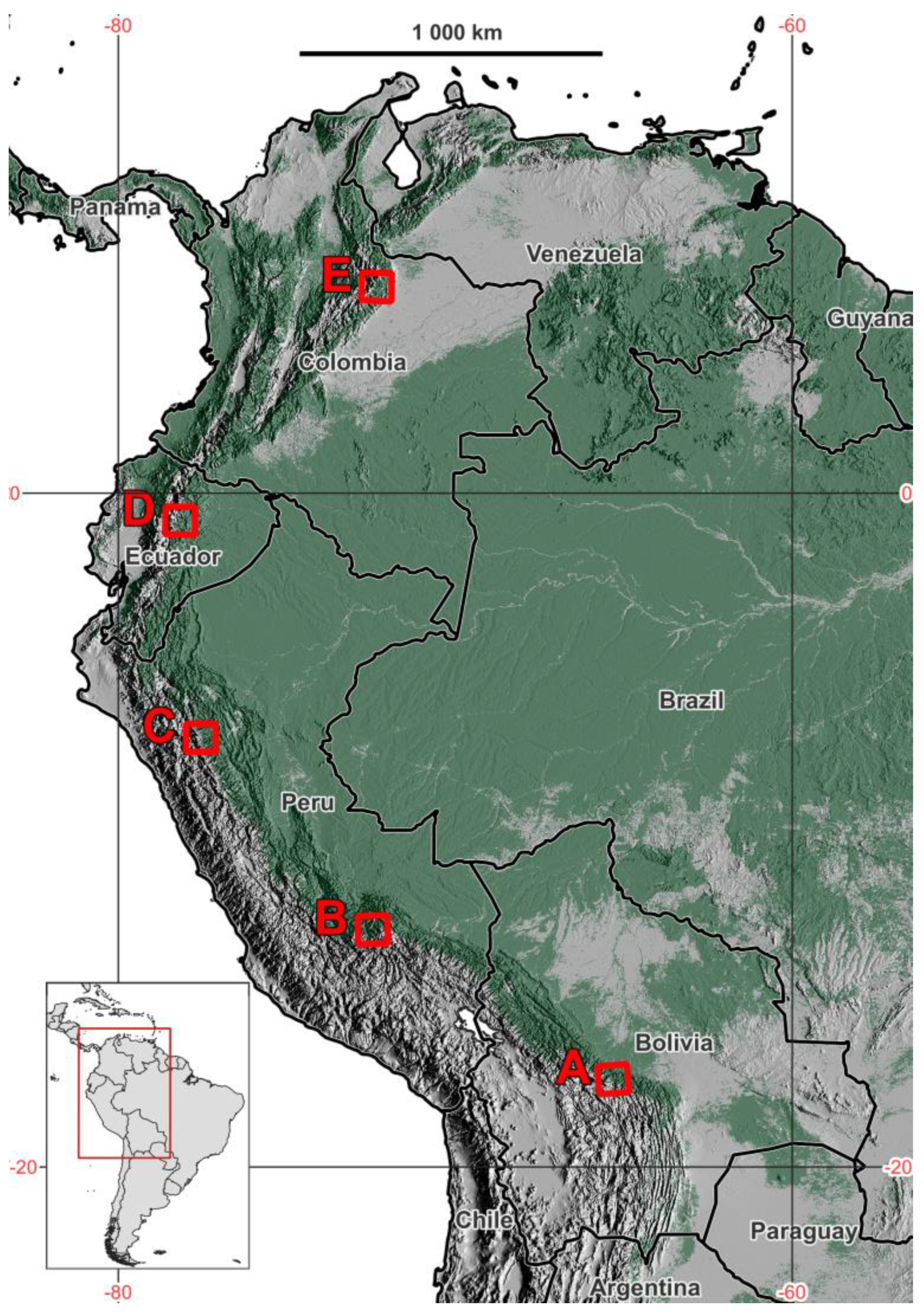
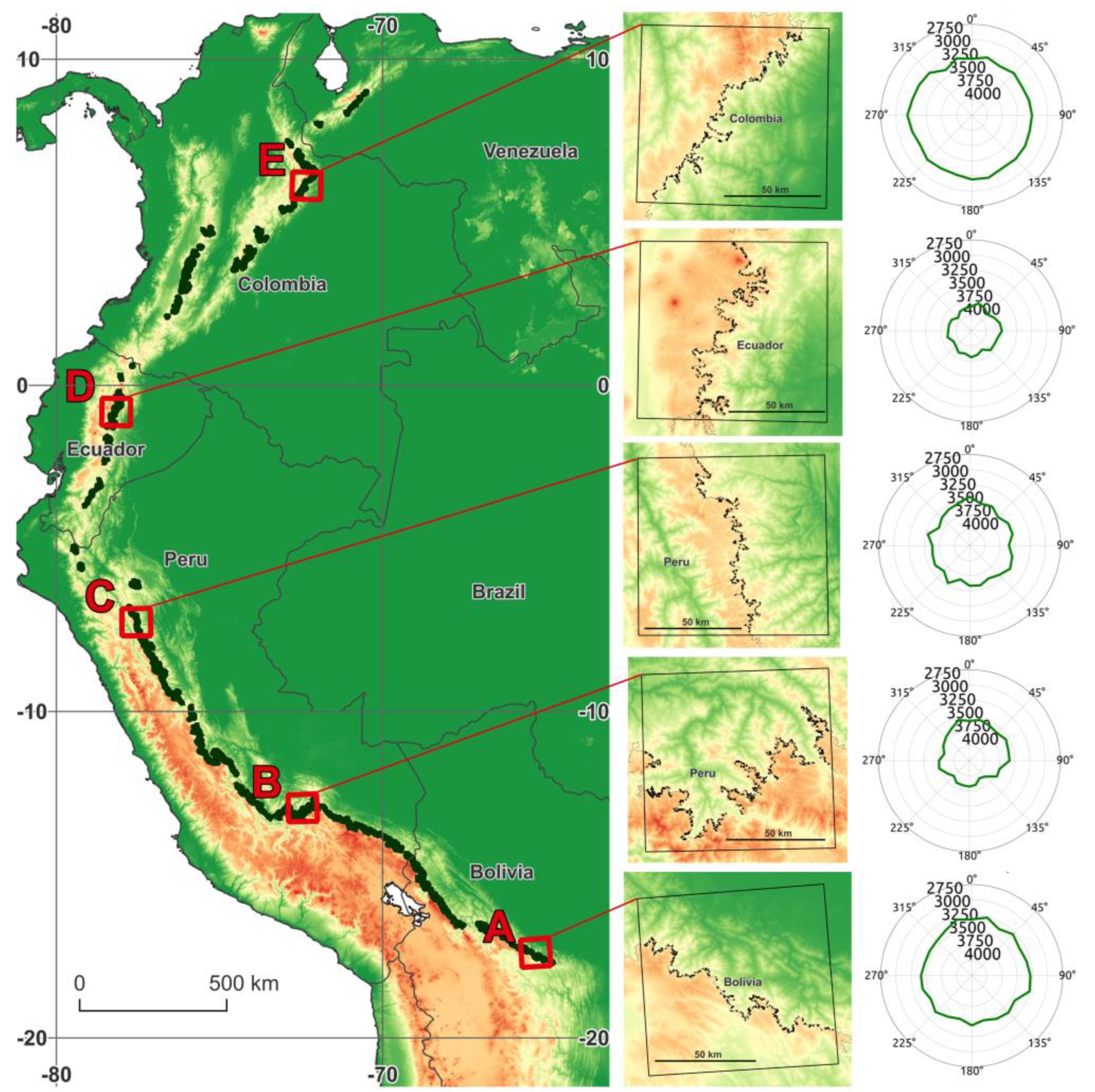
2.1. Study Area

This analysis is focused on the eastern Andean treeline (EATL) between 9°N and 18°S, spanning through western Venezuela, Bolivia, Ecuador, and Peru (Figure 1). In the north, the EATL ends where there is no more land area above the forests’ thermal limit. In the south, the boundary is set by the transition from evergreen broadleaf forests to deciduous broadleaf forests at the eastern Andean ‘elbow’ (~18°S), where the orientation of the mountain range changes abruptly from SE to S.
Although the broad evergreen broadleaf forest class appears to form a large and consistent expanse between the majority of the eastern Andes and the eastern edge of the continent (with the exception of adjacent savannas in northern Columbia and in Venezuela), in practice, the broadleaf humid tropical forests of the lowlands are distinct from the broadleaf montane forests (generally above 1500 m; [24]) in terms of species composition, posture, and biomass. At the treeline, forests generally represent the distinct Tropical Montane Cloud Forest, with many endemic species, and relatively low posture and aboveground biomass. Apart from the altitudinal vegetation gradient in the research area, there is also a latitudinal gradient of increasing forest seasonality away from the equator, which can be linked to changes in both precipitation and temperature.
Vegetation above the treeline, generally above 3200–3500 m, constitutes mainly montane grasslands and some shrublands. Within the Andean altiplano, from below the ‘elbow’ and up to ~13°S in Peru, it forms a distinct biome called puna. To the north from the altiplano, land above 3500 m is less abundant, and it disappears almost entirely in northern Peru around 6°S, in the region called Huancabamba Depression, covered with the distinct Marañón dry forests. The high-altitude vegetation above forests in neighboring Ecuador is a distinct Páramo, covering the largest area in that country, but also present in Colombian Cordillera Oriental and Venezuelan Cordillera de Mérida.
A more detailed assessment of the three-dimensional structure of the treeline was conducted within five focus regions (marked A–E in Figure 1), evenly distributed across the research area. Each focus region is ~100 km wide and represents a distinct vegetation type and direction of the treeline.

2.2. Materials

The first, large-scale, stage of the analysis was conducted using a land cover map derived from Moderate Resolution Imaging Spectroradiometer (MODIS) data—MCD12Q1 [25]. Specifically, the latest available map was used, from 2021, with vegetation classified according to the LCCS1 FAO Land Cover Classification System (one of eight available). The product has a 463 m spatial resolution. Moreover, topography was characterized using NASA’s Shuttle Radar Topography Mission (SRTM) Version 3.0 Global 1 arc second dataset (SRTMGL1) [26].
The second stage, conducted at a finer spatial resolution, focused on five focus regions and utilized the Global Land Cover and Land Use Change dataset [27], based on Landsat Analysis Ready Data [23], to describe the presence of forest around the year 2020, at 30 m spatial resolution.
Finally, the Climatologies at High Resolution for the Earth’s Land Surface Areas—CHELSA [28] was used to characterize the climate in the vicinity of the treeline. Climatology in the period 1981–2010, at a spatial resolution of 30 arc sec (~1 km), comprising 12 monthly maps for each variable (daily mean air temperature at 2 m—TAS, daily minimum air temperature at 2 m—TASMIN, mean potential evapotranspiration—PET, and mean precipitation—PR), was chosen as the most appropriate for the task.

2.3. Methods

The first stage of the analysis aimed to map the location and continuity of the EATL across the tropical Andes. It was conducted using the QGIS software (versions 2.18.14 and 3.22.14). After visual inspection against a high-resolution Microsoft Bing Maps satellite imagery background, the MCD12Q1 LCCS1 land cover map was re-classified into a forest-non-forest map. The vicinity of the EATL included classes 11 (evergreen needleleaf forests—sparsely represented), 12 (evergreen broadleaf forests—abundant), and 21 (open forest), which were merged into one broad “forest mask” class. Class 14—deciduous broadleaf forests, generally abundant below the study area and used to set its southern limit—was also present within the tropical zone, but only in a few small and primarily non-forest areas, and it was excluded from the analysis.
In order to map the upper boundary of montane forests, the forest mask was first constrained to areas above 1000 m.s.l. within the Andean massif. Then, the forest mask was vectorized, and small “islands” sized 1–4 pixels (21.5–85.9 ha) were removed since the goal was to map the continuous forest extent. Subsequently, the forest mask polygons were converted to lines and then clipped with polygons depicting Andean areas above 1500 m.s.l. (roughly the boundary of the Tropical Montane Cloud Forest). As a result, all boundaries below 1500 m.s.l. were removed. The last step of the regional analysis focused on continuous lines in regions above 3000 m.s.l., where the presence of a forest boundary at its climatic limit can be expected. Through visual inspection, a number of anthropogenic boundary lines near agricultural areas were removed, including “inverted” treelines that form on the slopes of deforested valleys. Moreover, crossings over were cut off, as were a small number of areas where visual inspection was not possible due to clouds in the Microsoft Bing Maps record. The final set of treelines were smoothed using the Cartographic Line Generalization plugin (https://github.com/dtutic/CartoLineGen, accessed on 13 February 2023) and then converted to GIS points for which elevation and temperature data were extracted.
For the analysis within the focus regions, the high-resolution forest mask from the Global Land Cover and Land Use Change dataset for the year 2020 was cropped to match the extent of the focus regions. The resulting masks were filtered with the GDAL sieve tool (https://gdal.org/programs/gdal_sieve.html, accessed on 13 February 2023) in order to remove any features smaller than 10 pixels, which in turn highlighted the larger areas of continuous forest. In order to represent the thermal envelope of the treeline, the 12 monthly coverages of the CHELSA minimum monthly temperature climatology (TASMIN) were converted into one coverage with a minimum temperature in any month. The monthly mean temperature coverages were averaged into one annual coverage. Monthly potential evapotranspiration (PET) and precipitation (PR) were aggregated into annual values and used as the basis for the aridity index (PET/PR) [29]. Finally, the climatic variables and elevation maps, together with rasterized treelines, were clipped and resampled to match the grids of the forest masks.
The key part of the analysis, conducted within the five focus regions, was the automated delineation and assessment of altitudinal transects through a novel method implemented in Python code, available from the online repository at https://bitbucket.org/Zelazowski/treeline-scan, accessed on 13 February 2023.
The transects are defined as a set of pixels forming a straight line that is aligned with the general direction of the slope and cuts across an upper edge of a forest area. The necessary inputs are a forest mask and an elevation model. Additional maps can be provided in order to append their congruent values to all pixels of the transects. The topographic aspect is calculated automatically and split into eight 45° wide octants (N–S, NE–SW… NW–SE). Further processing is restricted to the range of elevations set prior to the run (here between 2500 and 4000 m). The local upper edge of the forest class (forest pixels that do not border any other forest pixels with higher elevation) serves as the midpoints of transects. For each n-th midpoint (n can be set; here n = 20), the direction of a transect is determined, and then a pre-defined number (here 21) of aligned pixels is designated symmetrically up- and down-hill from the midpoint. If the average aspect angle of all points within the transect places it in an octant different from the one used to determine its orientation, the transect is discarded. The geometries of the remaining transects are used to sample all input raster datasets. The resulting transects are stored in a GeoPackage file with two internal layers: points and lines. The points represent pixel centers and store the sampled raster values. The lines layer stores a set of general statistics, such as the average, minimum, and maximum values of each variable sampled with the transect, as well as a linear representation of the extents of transects.
Two strategies to research the EATL through automatically delineated transects were tested on the B focus region in Peru in order to select the most suitable approach to utilizing the new software (Figure 2). In the first (a) strategy, the input was a forest mask (based on the Global Land Cover and Land Use Change dataset; [27]) and the algorithm was allowed to define transects on any local elevation maxima (marked in red on the bottom-left map in Figure 2), and within the pre-defined range of permitted elevations. In the second (b) strategy, the transects were delineated only at the previously described preliminary treeline derived from the MODIS-based land cover map.

3. Results

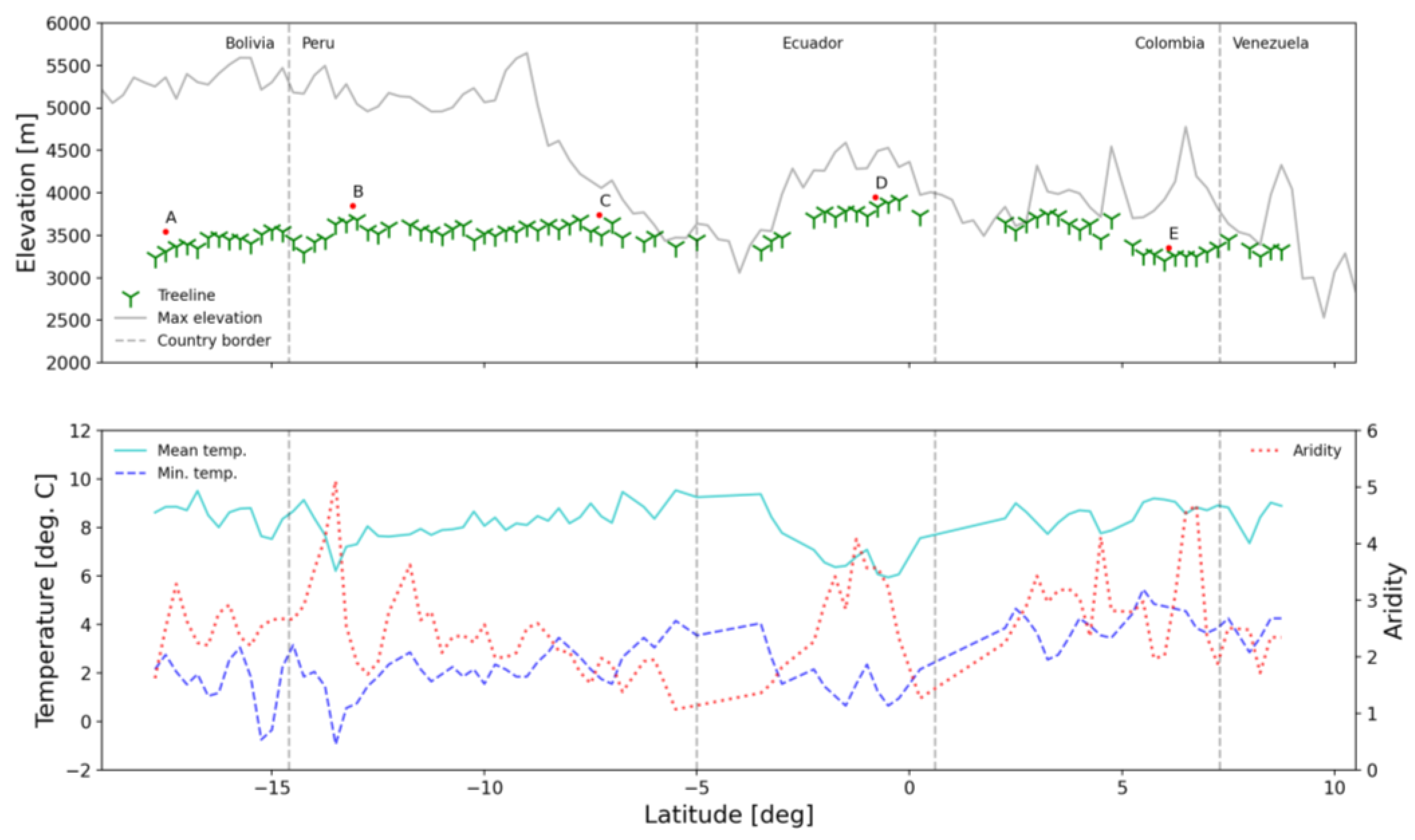
3.1. Contemporary Treeline Extent and Environmental Controls

The treeline defined in the regional analysis based on the MODIS-based land cover product MCD12Q1 spans ~4000 km in a straight line, while the actual length of the derived line is 12,117 km. Although the purpose was to extract a continuous western flank of the Amazon forests, wherever possible, in practice the line is not continuous in all of its extent, despite the fact that it is based on edges of relatively wide pixels (0.5 km-wide), adjacent with edges and/or corners. However, between the region around 18.5°S (the eastern Andean ‘elbow’), where the cordillera is locally fragmented and shifts to a more moderate climate regime with dominant deciduous forests, and around 6°S (near the Huancabamba Depression, also called Marañon Gap), where the massif’s maximum elevations drop to land above 3500 m, the forest frontier appears generally little fragmented, and therefore it is well represented by a continuous line (Figure 3). As visible on high-resolution imagery (Microsoft Bing Maps), the treeline in large parts of this region is also relatively discrete [30]. To this extent, starting in northern Bolivia, where the eastern Andean treeline’s altitude is ~3300 m, and throughout most of Peru, the treeline appears to generally have a consistent upper limit that depends on latitude, and increases towards the equator by ~30 m per geographic degree. The same trend continues after the Huancabamba Depression, where the treeline at one point reaches 3910 m. It should be noted that this altitudinal limit is independent of the amount of extra altitude available above the treeline.
The regular upper limit of the treeline supports the hypothesis that the upper forest limit is linked to temperature, which is generally strongly tied to both latitude and altitude. However, in the case of each presented temperature regime aspect, there is an area, at either end of the presented region, where forest occurs significantly below the margin specified with the linear trend. Specifically, the EATL in Bolivia appears to be placed in a climate regime with elevated annual mean temperatures, while the EATL in Colombia and Venezuela are in regimes with elevated minimum temperatures. Considering the amount of noise in the record, it is difficult to speculate which temperature metric performs better, although the mean temperature appears more stable. It is worth noting that the mean annual temperature is on average ~9.5 °C, which is three degrees higher than the 6.4 ± 0.4 °C seasonal mean air temperature limit described by [8]. Such a temperature difference translates to adiabatic cooling due to an altitude difference of ~500 m. Only in equatorial Ecuador does the EATL seem to be placed near the 6.4 °C limit.
The range of the aridity index values congruent with the treeline is relatively wide, but it is fully above the 0.65 threshold of the humid climate [29], even at the driest point, which falls within the Huancabamba Depression. Therefore, it can be concluded that water availability is probably not a factor limiting the altitudinal extent of the treeline.
From the Huancabamba Depression, the EATL loses its continuity, mainly due to forest fragmentation but also a lack of available land above the climatic limit. In this stretch, many parts of the initial EATL definition have been removed as, upon inspection, they appeared to be purely anthropogenic. The most abundant cases were the borders between agricultural land and either Páramo or the montane forest is Colombia, or the “inverted treelines” in Peru, emerging after deforestation from valley bottoms. It is also worth noting that between 2°N and 4.7°N, the record takes into account the Colombian Cordillera Central, which runs to the west from the Colombian Cordillera Oriental and parallel to it, and is therefore less available to the Amazonian flora. Despite the much greater fragmentation and smaller availability of suitable parts of the massif, the EATL north from the equator also appears to follow an elevational gradient that is twice as strong as the southern one (~60 m per geographic degree).

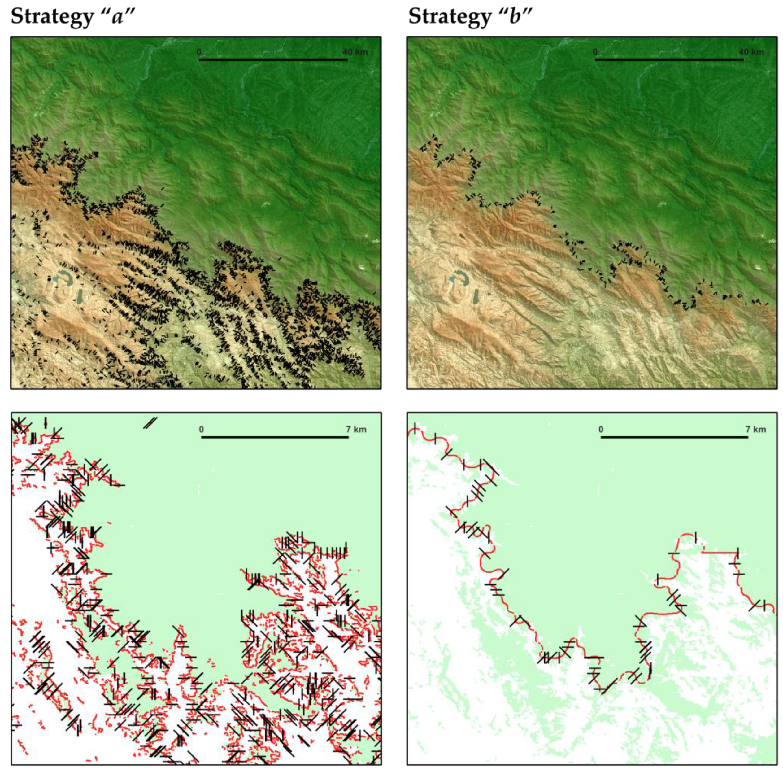
3.2. Assessment of Strategies for Automated Sampling with Transects

The two strategies considered for researching the EATL through automatically delineated transects yielded contrasting preliminary results.
It can be seen that the “a” strategy (Figure 2, left), in which the transects are delineated on any forested local elevation maxima in the region, but only within the pre-defined range of mountainous elevations, overall produces many more transects. This could potentially benefit the statistical robustness of the result. However, the transects are dispersed throughout a wide stretch of the landscape, and therefore they are not a robust representation of the actual frontier. Moreover, the detected forest fringes belong to different categories, including ones of purely anthropogenic origin, whereas in this project the focus has been on the natural EATL. A validation effort (inspection of fine-resolution imagery) in the case of this strategy would be prohibitively substantial. Nevertheless, for a broader study of any treelines in the landscape, the “a” strategy could be suitable.
In contrast, in the case of the “b” strategy (Figure 2, right), the transects were delineated only at the previously described MODIS-based treeline. For this reason, the “b” strategy was chosen as more appropriate to fulfil the set goal—to characterize the treeline, which forms the western frontier of the Amazonian evergreen forests. However, it should be noted that when the software was used according to the “a” strategy, a substantial portion of delineated transects (32%) were automatically placed in the vicinity of the MODIS-based treeline, which constitutes only 14% of the land area within the eligible elevation range.

3.3. Insight from Elevational Transects

Five focus regions were analyzed with the transect-delineating software, according to the “b” strategy. Each region is constrained by a ~100 km wide box. The actual length of the contained treeline varies considerably between the focus regions (Table 1), and together they represent 18% of the whole treeline delineated along the tropical zone (2221 km out of 12,117 km).
Treeline elevation followed the same trends as described for the whole region, which is to be expected since the two types of measurement are not independent. Nevertheless, on the scale of individual transects, in the cases where the elevation of the MODIS-based treeline was underestimated, the sampling of the fine-resolution forest mask allows us to compensate for this, at least in part. Since the transects were 21 pixels long, 10 pixels ought to sample land above the preliminary regional treeline, which, at Landsat’s resolution, translates to an altitude correction potential of up to 280 m. Indeed, in all of the focus regions, the treeline elevation detected with the software for transect delineation is higher than in the regional analysis, on average by 172 m, and a maximum of 201 m in the Peruvian site (Table 1 and Figure 3). These differences are below the above-stated detection limit, which asserts that the detected altitudes are near the actual treeline (i.e., as depicted in the fine-resolution Landsat-based product), although some individual transects certainly have not reached the highest local forest, as can be judged from the standard deviation of the mean (Table 1).
Since the temperature record is of relatively low resolution (1 km, resampled to match the 30 m SRTM layer), the new approach has not yielded new information as regards the climatological niche, while it has confirmed that only one EATL region in Ecuador is in the vicinity of the mean temperature threshold established in [8].
A more original contribution from the transect-based analysis concerns the three-dimensional nature of the forest extent, as it revealed that the treeline elevation depends on the hillside aspect (Table 1). Looking from the perspective of the overall direction of the massif’s exposure to open terrain (Figure 4, five inset maps), its northernness appears to be linked with the discrepancy in EATL altitude along the SW-NE axis (calculated after excluding four borderline aspect bins). In four focus regions, the treeline on the SW slopes has a higher altitude, with the maximum discrepancy occurring in the most north-facing Peruvian region (201 m). The SE-facing (i.e., with the least northern exposure) Columbian site is the only one located in the northern hemisphere, which probably explains why its treeline is reaching a higher elevation (by 63 m) on the NE slopes. Interestingly, along the N–S axis, the difference in treeline elevation is negligible (below 20 m in all of the focus regions), despite the highest contrast in the potential insolation of the slopes facing these directions.

4. Discussion

This study analyzed a set of datasets based on satellite remote sensing, as well as climate model results, with the aim of examining the extent of the continuous treeline in a ~30° latitude-long region spanning through Bolivia, Peru, Ecuador, and Venezuela. We have shown that in over half of the region, the treeline reaches an altitudinal limit that increases towards the equator by ~30 m and ~60 m per geographic degree in the south and north, respectively.
The presence of a clear, latitude-dependent gradient of maximum treeline elevation suggests that the potential forest extent is dictated by the temperature regime, as temperature is the only factor that changes with elevation and latitude with comparable consistency. It is unlikely that such a pattern could be explained by anthropogenic pressure, unless it is somehow controlled by elevation or temperature. This generally conforms to the theory presented by Korner and Paulsen [31], stating that the treeline extent is controlled by a temperature threshold of ~7 °C (later refined to 6.4 ± 0.4 °C), below which vascular plants are unable to grow. However, the annual mean temperature at the treeline presented in this study is up to three degrees higher than the proposed threshold, and the link is not as strong as reported in the literature. One possible explanation for this discrepancy could be the relatively more significant role of infrequent frost events, as suggested previously [7,8], which are particularly difficult to depict adequately in long-term climatology.
Our results contradict the theory stating that all of the Andean treeline extent is shaped by anthropogenic influences [13,32,33]. We show that the disturbance is not omnipresent across the region, but that in parts of the Andes, the treeline depression is indeed substantial and widespread. Extrapolation based on those regions could lead to an overestimation of the overall human impact.
In the relatively undisturbed parts, where the treeline appears not to be depressed, it might play an important role in the formation of climate refugia for the forest-dwelling species, as has already been reported [6]. Moreover, in these regions, climate warming is more likely to cause an upward shift, as reported in a number of locations globally [7], while evidence for South America is still scarce. Nevertheless, the concept of climate refugia should be seen in a broader context, which includes other aspects of climate, such as moisture availability—key for the TCMF—and that the encroached land might also represent a scarce biodiversity resource, such as in the case of páramo [8]
Sources of uncertainty in this study can be split into natural and artificial. One major natural uncertainty stems from the definition of the treeline. It should be noted that the theoretical framework and nomenclature in this area of research are still evolving [30]. In general, a treeline is either a sharp transition between biomes or an ecotone, and its appearance depends on the spatial scale considered. Here, treeline has been treated as discrete, and in many steep parts of the Andes, it is indeed close to such a form. Nevertheless, the level of “discreteness” has not been considered in this study. As pointed out in [10], treeline elevation is also a function of forest form. Some trees are able to reach higher elevations in a characteristic dwarfed form (Krumholtz treeline), which allows them to limit their contact (“coupling”) with the free atmosphere. Ref. [33] documented that in the Andes, some treeline species can be found as shrubs, trees, or scandent plants depending on local conditions, demonstrating the potential for great plasticity in growth forms within single species. Such morphological plasticity may make the climatological thresholds for forest existence more elusive.
Regarding the artificial sources of uncertainty, these are mainly linked to the datasets used in the study. For example, our forest mask was based on a discrete land cover product, which by necessity oversimplifies reality. Alternatively, the analysis could be based on a product depicting a continuous variable, such as the Global, 30 m Resolution Continuous Fields of Tree Cover [34]. This would allow for more flexibility in the definition of the forest boundary; nevertheless, the concept of the treeline itself is discrete; therefore, ultimately, any continuous variable would need to be converted to a discrete one. Another key dataset used here—the latest 30 m SRTM elevation data—in a remote region like the Andes, is likely to significantly exceed the stated benchmark of an absolute vertical accuracy of RMSE of 10 m. Ref. [35], while each 10 m difference in elevation might translate to ~0.06 °C difference in the inferred temperature envelope.
Yet, probably the most significant uncertainty is linked to maps describing climate, and for two reasons. First, although, according to [28], the CHELSA dataset performs better than WorldClim [36] at representing orographic patterns in topographically complex terrain, these fine-resolution maps are based on statistical downscaling of low-resolution climate models, and their quality is limited by the low number of weather stations available in the region; as a result, its climatic complexity is likely to be poorly represented. Moreover, the resolution of the dataset is 1 km—much lower than the fine resolution considered in the second part of the analysis, which might as well be a source of bias of magnitude comparable to the discrepancies reported here, despite the applied bilinear re-sampling.
Finally, the reported temperature estimates based on treeline extracted from classified MODIS-based imagery could introduce a positive bias linked to the relatively low resolution (0.5 km) of the dataset, despite the fact that pixel edges adjacent to higher elevations were used in the study. It can be expected that in such a dataset, some pixels representing the actual treeline will be classified as grassland or shrubland if the forest signal is not prevailing.
It can be argued that the chosen strategy (“b”) for sampling with transects, in which they are delineated only at the pre-defined treeline, has the advantage of being able to take into account the combined definitions of the forest frontier, as seen in the regional (MODIS) and local (Landsat) perspectives and resolutions. While the MODIS-based description offers more insight into biogeographical perspectives (ecosystem types and landscape continuity on a continental scale), it is much less accurate spatially. As reported in the results, this inaccuracy is then at least partially corrected when the forest edge is re-defined in the fine-resolution pixels of each transect, which also results in the upward correction. It can therefore be concluded that the final result is the most consistent western forest frontier, defined from a regional perspective and described with locally available fine detail. The emergence of the consistent longitudinal gradient of the treeline elevation serves as a first-order validation of the approach presented in this study.
While the presented method opened the door to an efficient assessment on a near-continental scale, there is certainly potential to further improve its scalability. In particular, the first part of the analysis could also take the form of a computer program with an implemented set of rules, allowing it to perform a first-order assessment on a large scale.
The approach to addressing the 3D mountainous environment through elevational transects allowed us to reveal a more nuanced aspect-dependent pattern of the treeline range. Specifically, there is a bias in altitudinal extent within slopes perpendicular to the NE–SW axis. According to a global analysis [37], vegetation cover is higher on pole-facing slopes in 74% of terrain exhibiting topographic asymmetry, including in the Andes. The discrepancy is generally driven by the smaller exposure to direct insolation. This analysis has not reproduced such N–S asymmetry, but it did uncover a similar phenomenon occurring along the axis shifted to the east. Moreover, the magnitude of the asymmetry appeared to be correlated with the “northernness” of the overall massif direction; however, the second-best fitting explanation is simply the distance from the equator (although in this case, the order of the two furthest sites is reversed). Perhaps the varying exposure to the lowland in the east and its air masses (“easternness”) is linked to some of the unexplained results, such as the tilted axis across which treeline elevations are the most contrasting, and the particularly strong asymmetry of the Peruvian site at 13°S. Another potential explanation is that strong topographic shadows can introduce a bias, as the shadowed land is more likely to be classified as dark, dense forest. The fact that treeline elevations consistently appear higher in the west, while Landsat imagery is acquired when the land is illuminated by the morning sun in the east, gives some plausibility to this theory. There are certainly many more phenomena that can be addressed with the described toolset to improve our understanding of treeline dynamics or mountainous ecotones in general. For example, a multi-temporal analysis could help to test hypotheses around the already mentioned advancing of treelines with climate change. Moreover, a number of studies reported an increasing robustness of forests at the treeline, which is another aspect of their response to climate change [38], although relatively subtle, which might be less reported in the literature for this very reason (but see, for example, [39,40]). Studying these phenomena, and their possibly elusive spatio-temporal pattern, might require using continuous variables as input, such as the original Landsat signal or Continuous Fields of Tree Cover [34].

5. Conclusions

This study delineated the eastern Andean treeline in Bolivia, Peru, Ecuador, and Venezuela between 9°N and 18°S, and showed that in over half of its extent, the treeline reaches a consistent altitudinal limit that increases towards the equator by ~30 m and ~60 m per geographic degree in the south and north, respectively. The limit appears to be determined by the temperature regime, although the link is not as strong as reported in some literature (notably [9]). It can be concluded that in these relatively undisturbed parts, the EATL is likely to be able to adapt to climate change and play a part in the formation of climate refugia for forest-dwelling species. In the rest of the region, the treeline is substantially depressed or absent due to either anthropogenic pressure (fire and/or cattle ranching) or a dip in the cordillera’s elevation.
For the EATL assessment on a local scale and to address the three-dimensional nature of environmental change in mountainous environments, we have used a novel method of automated delineation and assessment of altitudinal transects, which revealed a more nuanced aspect-dependent pattern of treeline position. Specifically, there is a discrepancy in the EATL altitude along the SW-NE axis, with trees reaching higher elevations on the pole-facing slopes. We conclude that the applied dual-scale approach with automated mass transect sampling allows for an improved understanding of treeline dynamics.

Author Contributions

Conceptualization, P.Z., Y.M. and S.J.; methodology, P.Z. and S.J.; software, S.J.; validation, P.Z. and S.J.; formal analysis, P.Z. and S.J.; investigation, P.Z. and S.J.; resources, K.J.F.; data curation, P.Z. and S.J.; writing—original draft preparation, P.Z., Y.M. and K.J.F.; writing—review and editing, P.Z., Y.M., K.J.F. and S.J.; visualization, P.Z.; supervision, Y.M. and K.J.F.; project administration, P.Z.; funding acquisition, P.Z. All authors have read and agreed to the published version of the manuscript.

Funding

This work was funded by the National Science Centre, Poland, under research project no UMO-2014/13/D/ST10/00022.

Data Availability Statement

Software for computing elevational transects, together with sample data from this study, can be accessed at https://bitbucket.org/Zelazowski/treeline-scan, accessed on 13 February 2023.

Acknowledgments

All the authors would like to acknowledge the role of The Andes Biodiversity and Ecosystems Research Group (ABERG) in the formulation of this research project. P. Zelazowski would like to thank Jakub Styczeń for the introduction to new analytical tools.

Conflicts of Interest

The authors declare no conflict of interest. The funders had no role in the design of the study; in the collection, analyses, or interpretation of data; in the writing of the manuscript; or in the decision to publish the results.

References

  1. Myers, N.; Mittermeier, R.A.; Mittermeier, C.G.; da Fonseca, G.A.B.; Kent, J. Biodiversity Hotspots for Conservation Priorities. Nature 2000, 403, 853–858. [Google Scholar] [CrossRef] [PubMed]
  2. Pabón-Caicedo, J.D.; Arias, P.A.; Carril, A.F.; Espinoza, J.C.; Borrel, L.F.; Goubanova, K.; Lavado-Casimiro, W.; Masiokas, M.; Solman, S.; Villalba, R. Observed and Projected Hydroclimate Changes in the Andes. Front. Earth Sci. 2020, 8, 61. [Google Scholar] [CrossRef]
  3. Vuille, M.; Francou, B.; Wagnon, P.; Juen, I.; Kaser, G.; Mark, B.G.; Bradley, R.S. Climate Change and Tropical Andean Glaciers: Past, Present and Future. Earth-Sci. Rev. 2008, 89, 79–96. [Google Scholar] [CrossRef]
  4. Morueta-Holme, N.; Engemann, K.; Sandoval-Acuña, P.; Jonas, J.D.; Segnitz, R.M.; Svenning, J.-C. Strong Upslope Shifts in Chimborazo’s Vegetation over Two Centuries since Humboldt. Proc. Natl. Acad. Sci. USA 2015, 112, 12741–12745. [Google Scholar] [CrossRef] [PubMed]
  5. Colwell, R.K.; Brehm, G.; Cardelús, C.L.; Gilman, A.C.; Longino, J.T. Global Warming, Elevational Range Shifts, and Lowland Biotic Attrition in the Wet Tropics. Science 2008, 322, 258–261. [Google Scholar] [CrossRef] [PubMed]
  6. Feeley, K.J.; Silman, M.R.; Bush, M.B.; Farfan, W.; Cabrera, K.G.; Malhi, Y.; Meir, P.; Revilla, N.S.; Quisiyupanqui, M.N.R.; Saatchi, S. Upslope Migration of Andean Trees. J. Biogeogr. 2011, 38, 783–791. [Google Scholar] [CrossRef]
  7. Harsch, M.A.; Hulme, P.E.; McGlone, M.S.; Duncan, R.P. Are Treelines Advancing? A Global Meta-Analysis of Treeline Response to Climate Warming. Ecol. Lett. 2009, 12, 1040–1049. [Google Scholar] [CrossRef]
  8. Helmer, E.H.; Gerson, E.A.; Baggett, L.S.; Bird, B.J.; Ruzycki, T.S.; Voggesser, S.M. Neotropical Cloud Forests and Páramo to Contract and Dry from Declines in Cloud Immersion and Frost. PLoS ONE 2019, 14, e0213155. [Google Scholar] [CrossRef]
  9. Paulsen, J.; Körner, C. A Climate-Based Model to Predict Potential Treeline Position around the Globe. Alp. Bot. 2014, 124, 1–12. [Google Scholar] [CrossRef]
  10. Körner, C. The Cold Range Limit of Trees. Trends Ecol. Evol. 2021, 36, 979–989. [Google Scholar] [CrossRef]
  11. Kessler, M.; Böhner, J.; Kluge, J. Modelling Tree Height to Assess Climatic Conditions at Tree Lines in the Bolivian Andes. Ecol. Model. 2007, 207, 223–233. [Google Scholar] [CrossRef]
  12. Sarmiento, G.; Pinillos, M. The Tropical Alpine Treeline: A Case Study of a Changing Ecosystem Boundary. In Applying Ecological Knowledge to Land use Decisions; Inter-American Institute for Global Change Research: Montevideo, Uruguay, 2008; pp. 111–122. [Google Scholar]
  13. Sarmiento, F.O.; Frolich, L.M. Andean Cloud Forest Tree Lines. Mt. Res. Dev. 2002, 22, 278–287. [Google Scholar] [CrossRef]
  14. Lutz, D.A.; Powell, R.L.; Silman, M.R. Four Decades of Andean Timberline Migration and Implications for Biodiversity Loss with Climate Change. PLoS ONE 2013, 8, e74496. [Google Scholar] [CrossRef] [PubMed]
  15. Young, K.R.; Ponette-González, A.G.; Polk, M.H.; Lipton, J.K. Snowlines and Treelines in the Tropical Andes. Ann. Am. Assoc. Geogr. 2017, 107, 429–440. [Google Scholar] [CrossRef]
  16. Chacón-Moreno, E.; Rodríguez-Morales, M.; Paredes, D.; Suárez del Moral, P.; Albarrán, A. Impacts of Global Change on the Spatial Dynamics of Treeline in Venezuelan Andes. Front. Ecol. Evol. 2021, 9, 615223. [Google Scholar] [CrossRef]
  17. Holtmeier, F.K.; Broll, G.E. Treeline Advance—Driving Processes and Adverse Factors. Landsc. Online 2007, 1, 1–33. [Google Scholar] [CrossRef]
  18. Rita, A.; Bonanomi, G.; Allevato, E.; Borghetti, M.; Cesarano, G.; Mogavero, V.; Rossi, S.; Saulino, L.; Zotti, M.; Saracino, A. Topography Modulates Near-Ground Microclimate in the Mediterranean Fagus Sylvatica Treeline. Sci. Rep. 2021, 11, 8122. [Google Scholar] [CrossRef]
  19. Quadri, P.; Silva, L.C.R.; Zavaleta, E.S. Climate-Induced Reversal of Tree Growth Patterns at a Tropical Treeline. Sci. Adv. 2021, 7, eabb7572. [Google Scholar] [CrossRef]
  20. Pepin, N.; Bradley, R.S.; Diaz, H.F.; Baraer, M.; Caceres, E.B.; Forsythe, N.; Fowler, H.; Greenwood, G.; Hashmi, M.Z.; Liu, X.D.; et al. Elevation-Dependent Warming in Mountain Regions of the World. Nat. Clim. Chang. 2015, 5, 424–430. [Google Scholar] [CrossRef]
  21. Tovar, C.; Carril, A.F.; Gutiérrez, A.G.; Ahrends, A.; Fita, L.; Zaninelli, P.; Flombaum, P.; Abarzúa, A.M.; Alarcón, D.; Aschero, V.; et al. Understanding Climate Change Impacts on Biome and Plant Distributions in the Andes: Challenges and Opportunities. J. Biogeogr. 2022, 49, 1420–1442. [Google Scholar] [CrossRef]
  22. Storey, J.C.; Rengarajan, R.; Choate, M.J. Bundle Adjustment Using Space-Based Triangulation Method for Improving the Landsat Global Ground Reference. Remote Sens. 2019, 11, 1640. [Google Scholar] [CrossRef]
  23. Potapov, P.; Hansen, M.C.; Kommareddy, I.; Kommareddy, A.; Turubanova, S.; Pickens, A.; Adusei, B.; Tyukavina, A.; Ying, Q. Landsat Analysis Ready Data for Global Land Cover and Land Cover Change Mapping. Remote Sens. 2020, 12, 426. [Google Scholar] [CrossRef]
  24. Young, K.R.; Leon, B. Distribution and Conservation of Peru’s Montane Forests: Interactions between the Biota and Human Society. In Tropical Montane Cloud Forests; Springer: Cham, Switzerland, 1993; pp. 237–246. [Google Scholar]
  25. Sulla-Menashe, D.; Gray, J.M.; Abercrombie, S.P.; Friedl, M.A. Hierarchical Mapping of Annual Global Land Cover 2001 to Present: The MODIS Collection 6 Land Cover Product. Remote Sens. Environ. 2019, 222, 183–194. [Google Scholar] [CrossRef]
  26. Farr, T.G.; Rosen, P.A.; Caro, E.; Crippen, R.; Duren, R.; Hensley, S.; Kobrick, M.; Paller, M.; Rodriguez, E.; Roth, L.; et al. The Shuttle Radar Topography Mission. Rev. Geophys. 2007, 45, 183. [Google Scholar] [CrossRef]
  27. Potapov, P.; Hansen, M.C.; Pickens, A.; Hernandez-Serna, A.; Tyukavina, A.; Turubanova, S.; Zalles, V.; Li, X.; Khan, A.; Stolle, F.; et al. The Global 2000–2020 Land Cover and Land Use Change Dataset Derived from the Landsat Archive: First Results. Front. Remote Sens. 2022, 3, 18. [Google Scholar] [CrossRef]
  28. Karger, D.N.; Conrad, O.; Böhner, J.; Kawohl, T.; Kreft, H.; Soria-Auza, R.W.; Zimmermann, N.E.; Linder, H.P.; Kessler, M. Climatologies at High Resolution for the Earth’s Land Surface Areas. Sci. Data 2017, 4, 170122. [Google Scholar] [CrossRef]
  29. Zomer, R.J.; Xu, J.; Trabucco, A. Version 3 of the Global Aridity Index and Potential Evapotranspiration Database. Sci. Data 2022, 9, 409. [Google Scholar] [CrossRef]
  30. Bader, M.Y.; Llambí, L.D.; Case, B.S.; Buckley, H.L.; Toivonen, J.M.; Camarero, J.J.; Cairns, D.M.; Brown, C.D.; Wiegand, T.; Resler, L.M. A Global Framework for Linking Alpine-Treeline Ecotone Patterns to Underlying Processes. Ecography 2021, 44, 265–292. [Google Scholar] [CrossRef]
  31. Korner, C.; Paulsen, J. A World-Wide Study of High Altitude Treeline Temperatures. J. Biogeogr. 2004, 31, 713–732. [Google Scholar] [CrossRef]
  32. Kok, K.V.; Kok, P.A.; Beukema, H. Effects of Cutting and Grazing on Andean Treeline Vegetation. In Biodiversity and Conservation of Neotropical Montane Forests; Churchill, S.P., Balslev, H., Forero, E., Luteyn, J.L., Eds.; New York Botanical Garden: New York, NY, USA, 1995. [Google Scholar]
  33. Sarmiento, F. Anthropogenic Change in the Landscapes of Highland Ecuador. Geogr. Rev. 2002, 92, 213–234. [Google Scholar] [CrossRef]
  34. Sexton, J.O.; Song, X.-P.; Feng, M.; Noojipady, P.; Anand, A.; Huang, C.; Kim, D.-H.; Collins, K.M.; Channan, S.; DiMiceli, C.; et al. Global, 30-m Resolution Continuous Fields of Tree Cover: Landsat-Based Rescaling of MODIS Vegetation Continuous Fields with Lidar-Based Estimates of Error. Int. J. Digit. Earth 2013, 6, 427–448. [Google Scholar] [CrossRef]
  35. Mukul, M.; Srivastava, V.; Mukul, M. Accuracy Analysis of the 2014–2015 Global Shuttle Radar Topography Mission (SRTM) 1 Arc-Sec C-Band Height Model Using International Global Navigation Satellite System Service (IGS) Network. J. Earth Syst. Sci. 2016, 125, 909–917. [Google Scholar] [CrossRef]
  36. Fick, S.E.; Hijmans, R.J. WorldClim 2: New 1-Km Spatial Resolution Climate Surfaces for Global Land Areas. Int. J. Climatol. 2017, 37, 4302–4315. [Google Scholar] [CrossRef]
  37. Smith, T.; Bookhagen, B. Climatic and Biotic Controls on Topographic Asymmetry at the Global Scale. J. Geophys. Res. Earth Surf. 2021, 126, e2020JF005692. [Google Scholar] [CrossRef]
  38. Grace, J.; Berninger, F.; Nagy, L. Impacts of Climate Change on the Tree Line. Ann. Bot. 2002, 90, 537–544. [Google Scholar] [CrossRef]
  39. Myneni, R.B.; Dong, J.; Tucker, C.J.; Kaufmann, R.K.; Kauppi, P.E.; Liski, J.; Zhou, L.; Alexeyev, V.; Hughes, M.K. A Large Carbon Sink in the Woody Biomass of Northern Forests. Proc. Natl. Acad. Sci. USA 2001, 98, 14784–14789. [Google Scholar] [CrossRef]
  40. Olthof, I.; Pouliot, D. Treeline Vegetation Composition and Change in Canada’s Western Subarctic from AVHRR and Canopy Reflectance Modeling. Remote Sens. Environ. 2010, 114, 805–815. [Google Scholar] [CrossRef]
Figure 1. Study area, encompassing the Northern Andes and the northern part of the Central Andes, where the tropical part of the eastern Andean treeline is located. The MODIS-based mask of evergreen deciduous forests is shown in green. A–E are focus regions.
Remotesensing 15 02679 g001
Figure 2. Two strategies to investigate the treeline position through automated delineation of transects. The top row shows transects against high-resolution Microsoft Bing Maps with an overlaid colored elevation map (SRTM). The bottom row shows transects against the forest mask derived from the Global Land Cover and Land Use Change dataset [27]. Elements marked in red—local elevation maxima within the forest mask (left) and the MODIS MCD12Q1 product-based treeline (right)—were used as anchors for transects.
Remotesensing 15 02679 g002
Figure 3. Eastern Andean treeline of evergreen broadleaf forests and corresponding information on topography, temperature, and aridity, across ~30 degrees of latitude. All data points represent 2.5 degree-wide bins. Red points marked A–E represent the average treeline elevation in the focus regions, estimated through automated transect sampling.
Remotesensing 15 02679 g003
Figure 4. Left: Eastern Andean treeline marked on the elevation model (SRTM). A–E are focus regions. Middle: Focus regions with marked elevational transects. Right: The dependence between the aspect of forested slopes and the treeline elevation within focus regions.
Remotesensing 15 02679 g004
Table 1. Characterization of the five focus regions within the tropical eastern Andean treeline.
CharacteristicFocus Region
ABCDE
Coordinates (midpoint)65.3°W, 17.5°S72.4°W, 13.1°S77.5°W, 7.3°S78.2°W, 0.8°S72.4°W, 6.1°N
CountryBoliviaPeruPeruEcuadorColumbia
Overall orientationN-E (28°)N (327°)E (78°)E (108°)S-E (129°)
Length [km]296754304489378
Elevation; avg. ± SD [m]3466 ± 1523766 ± 2003656 ± 1723878 ± 1303291 ± 158
Diff. from regional estimate [m]+211+243+154+140+112
SW-NE elev. diff. [m] 1272018150−63
Annual mean temp. [°C]9.13 ± 0.787.86 ± 1.008.91 ± 0.746.75 ± 0.659.48 ± 0.67
Annual min. temp. [°C]2.9 ± 0.922.07 ± 1.182.15 ± 0.691.8 ± 0.785.24 ± 0.74
Disclaimer/Publisher’s Note: The statements, opinions and data contained in all publications are solely those of the individual author(s) and contributor(s) and not of MDPI and/or the editor(s). MDPI and/or the editor(s) disclaim responsibility for any injury to people or property resulting from any ideas, methods, instructions or products referred to in the content.

