Article

An Enhanced Storm Warning and Nowcasting Model in Pre-Convection Environments

1
Key Laboratory of Cloud-Precipitation Physics and Severe Storms (LACS), Institute of Atmospheric Physics, Chinese Academy of Sciences, Beijing 100029, China
2
Cooperative Institute for Meteorological Satellite Studies, University of Wisconsin-Madison, Madison, WI 53706, USA
3
University of Chinese Academy of Sciences, Beijing 100049, China
4
National Satellite Meteorological Center, China Meteorological Administration, Beijing 100081, China
5
School of Atmospheric Sciences, and Guangdong Province Key Laboratory for Climate Change and Natural Disaster Studies, Sun Yat-sen University, Guangzhou 519082, China
6
Advanced Satellite Products Branch, STAR/NESDIS/NOAA, Madison, WI 53706, USA
7
Atlantic Oceanic Meteorological Laboratory (AOML)/NOAA, Miami, FL 33149, USA
*
Author to whom correspondence should be addressed.
Remote Sens. 2023, 15(10), 2672; https://doi.org/10.3390/rs15102672
Submission received: 14 April 2023 / Revised: 11 May 2023 / Accepted: 16 May 2023 / Published: 20 May 2023
(This article belongs to the Section Atmospheric Remote Sensing)

Abstract

:
A storm tracking and nowcasting model was developed for the contiguous US (CONUS) by combining observations from the advanced baseline imager (ABI) and numerical weather prediction (NWP) short-range forecast data, along with the precipitation rate from CMORPH (the Climate Prediction Center morphing technique). A random forest based model was adopted by using the maximum precipitation rate as the benchmark for convection intensity, with the location and time of storms optimized by using optical flow (OF) and continuous tracking. Comparative evaluations showed that the optimized models had higher accuracy for severe storms with areas equal to or larger than 5000 km2 over smaller samples, and loweraccuracy for cases smaller than 1000 km2, while models with sample-balancing applied showed higher possibilities of detection (PODs). A typical convective event from August 2019 was presented to illustrate the application of the nowcasting model on local severe storm (LSS) identification and warnings in the pre-convection stage; the model successfully provided warnings with a lead time of 1–2 h before heavy rainfall. Importance score analysis showed that the overall impact from ABI observations was much higher than that from NWP, with the brightness temperature difference between 6.2 and 10.3 microns ranking at the top in terms of feature importance.

1. Introduction

Severe convective storms such as thunderstorms, hailstorms and short-duration heavy rainfall are typical high-impact weather events that pose threats to life and property. With the relatively small spatial scale and rapid evolution of convective systems, it remains challenging for forecasters to accurately forecast the initiation and severity of convective storms. Local severe storms (LSS) are especially difficult to forecast as they are usually isolated and occur suddenly, with little direct impact from synoptic scales [1,2]. Therefore, it is very important to accurately predict the initiation process of local convection. However, as the specific details of the local convective initiation process are still not well simulated in numerical weather prediction (NWP) models, predicting the timing and location for the initial development of local severe storms using only NWP still has large uncertainties [3]. While radar observations play an important role in operational forecasts for tracking the intensity of convection, they do not provide enough information on convective initiation when used alone [4,5,6]. With fine spatial and temporal resolutions, geostationary satellite imagers have been widely used in storm identification and tracking [7,8,9,10,11], providing information conducive to convective initiation (CI) research.
Some objective methods for CI nowcasting have been developed using criteria from geostationary satellite observations. Roberts and Rutledge [6] found a drop in brightness temperature (BT) from the infrared (IR) window channel from 0 °C to −20 °C to be a precursor to storm initiation in radar-detected convective clouds. Mosher [12] developed the global convective diagnostic algorithm using the BT difference between the 11 µm and 6.7 µm bands to monitor thunderstorm convection from geostationary satellites. Multispectral information from geostationary operational environmental satellite (GOES) Imager observations, along with cloud tracking techniques, have been used by Mecikalski and Bedka [13] to establish a CI nowcasting approach with a set of interest fields. Validation of this algorithm, known as the satellite convection analysis and tracking (SATCAST) system, shows that good quality cumulus tracking is important for the algorithm to achieve better accuracy [14]. An enhanced version, SATCASTv2, was developed by Walker et al. [15] by changing the cloud tracking approach from single-pixel tracking to cloud-object tracking, where statistical skill results show overall improvements but vary by geolocation. Another CI system, the University of Wisconsin convective initiation (UWCI) algorithm, was developed with increased computational efficiency by calculating box-averaged cloud-top cooling rates and using 4 K per 15 min as a threshold to filter the candidates for nowcasting [16].
Apart from those CI systems with constant thresholds, modern advanced machine learning (ML) techniques have already been used for forecasting and nowcasting convection with promising results [17,18,19]. Random forest (RF) and neural network (NN) algorithms have proven to be useful in developing ML-based CI models with input from geostationary satellite observations in specific geographic regions [20,21,22,23]. Meanwhile, optical flow (OF) methods, widely used in computer vision, have also been found to be useful in nowcasting tasks as they promote flexibility in tracking candidates of small scales [22,24,25,26,27]. ProbSevere, a probabilistic model, was developed using naïve Bayesian classifiers to provide nowcasting results for different kinds of severe hazards via integrating multiple data sources including radar, lightning, NWP and satellite observations [28].
In contrast to the ProbSevere system, a storm tracking and nowcasting model known as storm warning in pre-convective environment (SWIPE), was developed by Liu et al. [29] using geostationary satellite multi-band IR measurements from Himawari-8, in combination with global numerical weather prediction (NWP) forecast data from the GFS (Global Forecast System). SWIPE was developed for the purpose of better utilizing geostationary satellite observations with high temporal and spatial resolutions to help identify potentially severe storms that may lead to severe rainfall and flooding events before convective systems are developed, especially the local storms that are difficult to predict from operational NWP models. Research studies and operational use have demonstrated that the SWIPE model is capable of capturing and nowcasting the severity of local burst storm systems characterized by the maximum rain rate in the pre-convection stages, with the advantage of detecting LSS occurrence and severity in the pre-convection stage before radar. This study will provide a US-based and enhanced version of SWIPE using tracked convective cases from the contiguous US (CONUS) using satellite observations from GOES-16, with an OF algorithm incorporated to overcome the limitations of the SWIPE algorithm.
The remainder of this paper is organized as follows. Section 2 introduces the data used in this study. Section 3 explains the algorithm for SWIPE methodologies to track convective cases and establish the dataset for ML training and validation, its limitations and the corresponding enhancements. The training and optimization of the RF prediction model, and the statistical validation results, along with the nowcasting application are presented and discussed in Section 4. Finally, a summary and discussion are provided in Section 5.

2. Data

Seven continuous months, from March to October 2018, of ABI CONUS data from GOES-16 were used to identify and track the convective samples for training the ML-based prediction model. GOES-16, the first satellite of the new-generation geostationary operational environmental satellite (GOES-R series), has a fine spatial resolution of 2 km at nadir for IR channels, and a fast scan rate of 5 min for CONUS [30]. ABI has 16 channels, 10 of which are IR channels with channel numbers from 7 to 16. All 10 IR channels were used in this study; in particular, the cooling rate of the brightness temperature from the 10.3 μm channel was used for storm identification and tracking, while the other channels contributed to forming the predictors of the model. More details on the description and usage of ABI’s channels can be found in previous papers [30,31].
In addition to geostationary satellite observations from ABI CONUS, NWP data from the Global Forecast System (GFS) was used to provide dynamic and environmental information about the atmosphere. Such information was not available from satellite observations due to cloud contamination. The NWP data with a spatial resolution of 0.5° × 0.5° and a 3-h time interval, on 26 vertical layers from 10 to 1000 hPa [32], can be obtained at four initial forecast times daily (0000, 0600, 1200 and 1800 UTC) from the National Oceanic and Atmospheric Administration (NOAA, https://www.ncdc.noaa.gov/data-access/model-data/model-datasets/global-forcast-system-gfs, accessed on 17 February 2022). Our goal was to use the dynamic and environmental information from the NWP forecast data as the background of the atmosphere to support nowcasting CI. Some parameters related to convective environments, such as lifted index (LI), total precipitable water (TPW) and K-index, were calculated and mapped to the observations of ABI via linear interpolation. Next, these parameters were put into the training as predictors in collocation with ABI variables.
Inherited from the original SWIPE model (SWIPEv1) [29], the enhanced model also focuses on nowcasting convective events that are associated with heavy precipitation, which may lead to flooding. According to the authors in [33], flooding is the leading cause of weather- and climate-hazard-related fatalities in North America. The gridded precipitation analysis data from the bias-corrected CMORPH (the Climate Prediction Center morphing technique), namely CMORPH version 1.0 CRT, was used in the study, with the maximum rainfall intensity functioning as the main indicator for truth in the training. This technique incorporates precipitation estimates derived from the passive microwave observations of the special sensor microwave imager (SSM/I), advanced microwave sounding unit (AMSU-B), advanced microwave scanning radiometer (AMSR-E) and TRMM microwave imager (TMI) aboard various low-orbit spacecraft, while the geostationary IR data are used only to derive the movement of precipitation systems [34]. In this study, we used CMORPH data covering a global area between the latitudes of 60°N and 60°S with a spatial resolution of 8 km (at the equator), and a 30-min time interval. The CRT product was adjusted from the original estimates to remove the bias through matching the PDF of daily CMORPH-RAW against the daily gauge analysis over land and with the pentad Global Prediction Climatology Project (GPCP) analysis over the ocean [35,36]. Previous validation studies of this product with gauge or radar observations have shown positive results [37,38,39,40]. This dataset with high spatial and temporal resolutions was used as the benchmark for classifying convective intensity in the training and validation process.

3. Methodology

3.1. SWIPE Model and Existing Issues

As is mentioned above, the original CI nowcasting framework SWIPEv1 was primarily developed through RF training from a collocated dataset of the advanced Himawari-8 imager (AHI, Advanced Himawari Imager) observations, GFS NWP forecast data and truth values of convective intensities derived from the CMORPH rain rate analysis [29]. Readers may refer to the original paper for details, and see Figure 3 of paper [29] for the flowchart of SWIPEv1 including the inputs, outputs, and modules of training and prediction. A brief introduction is provided in this section. The original algorithm consists of three major parts which are summarized as follows:
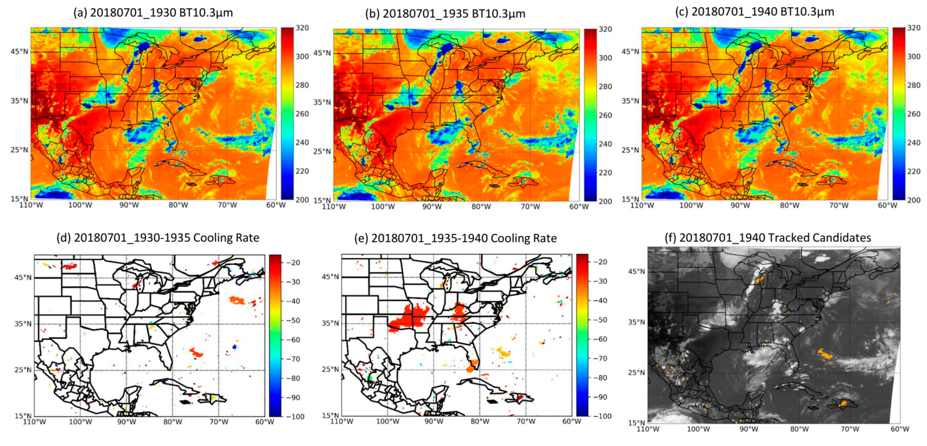
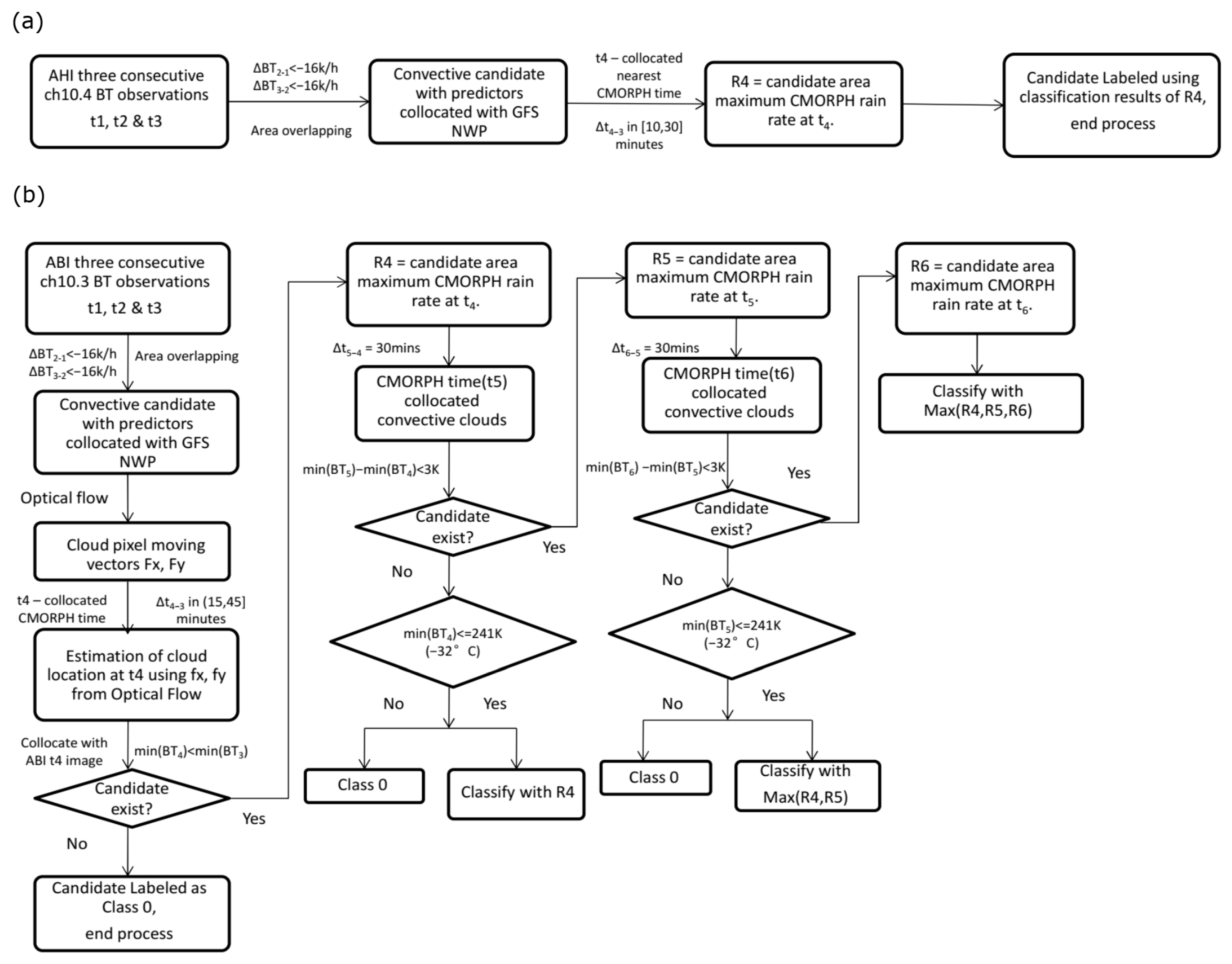
  • Convection identification and tracking. Possible clouds are firstly identified from BT observations of 10.4 μm as spatially continuous pixels with eight neighboring pixels that are no more than 273 K for each observation time of AHI. Candidate clouds with the potential of becoming convective are identified through two consecutive cooling rates calculated from the 10.4 µm band BT observations of three consecutive AHI images. The cooling rates are calculated from the equations below:
    R 1 = m i n ( B T A 2 , 1 , B T A 2 , 2   , , , B T A 2 , N 2 ) m i n ( B T A 1 , 1 , B T A 1 , 2   , , , B T A 1 , N 1 ) t 2 t 1  
    R 2 = m i n ( B T A 3 , 1 , B T A 3 , 2   , , , B T A 3 , N 3 ) m i n ( B T A 2 , 1 , B T A 2 , 2   , , , B T A 2 , N 2 ) t 3 t 2  
    For BTA2,1, the three subscripts A, 2 and 1 denote the candidate cloud, observation time and the pixel number within the cloud, respectively. N1, N2 and N3 represent the varying total pixel numbers of the tracked cloud at different consecutive times. Furthermore, t1, t2 and t3 are the times of the three AHI observations. To eliminate sudden noise and large-scale clouds that are associated with frontal cloud systems, clouds with a total pixel number less than 10 or greater than 50,000 are omitted. The corresponding clouds from different geostationary images are determined through an area overlapping method [41], and those clouds with both R1 and R2 reaching a cooling rate of 16 K/h are marked as candidates for potential convection and put into datasets for model training and validation. The cloud candidates that meet the consecutive cooling thresholds will be the targets of subsequent collocation and model development. This cooling rate requirement ensures that the SWIPE model is useful in the pre-convective environment or in the early stages of convection, where the storm just starts to develop and radar is less effective due to no or weak radar reflectivity.
  • Collocation of datasets. With tracked cases from geostationary observations, the BT variables from multiple channels of the cloud candidates are collocated with NWP variables and precipitation products to build a dataset for training and validation. For NWP, interpolations are made to match the grids to geostationary satellite pixels. For precipitation products, the analysis data immediately following the time a candidate is recognized is used to match the datasets as the truth value for classification [29]. Then, the convective candidates are divided into three intensity classes based on the maximum precipitation rate, and labeled accordingly for training and validation.
  • After the historical training dataset is built, the random forest (RF) algorithm [42] is used to train and optimize the convection intensity classification predictive model. During the training, a sample-balance technique is applied to avoid overfitting the model to the majority class (the weak class for this study) by adjusting the sample sizes of the three classes to 1:1:1 through under-sampling. Note that the weak class has a sample size that is 120 times that of the severe class.
While the current SWIPEv1 model has shown good efficiency in identifying and nowcasting the intensity level of local convective storms over East Asia, some limitations in the framework remain:
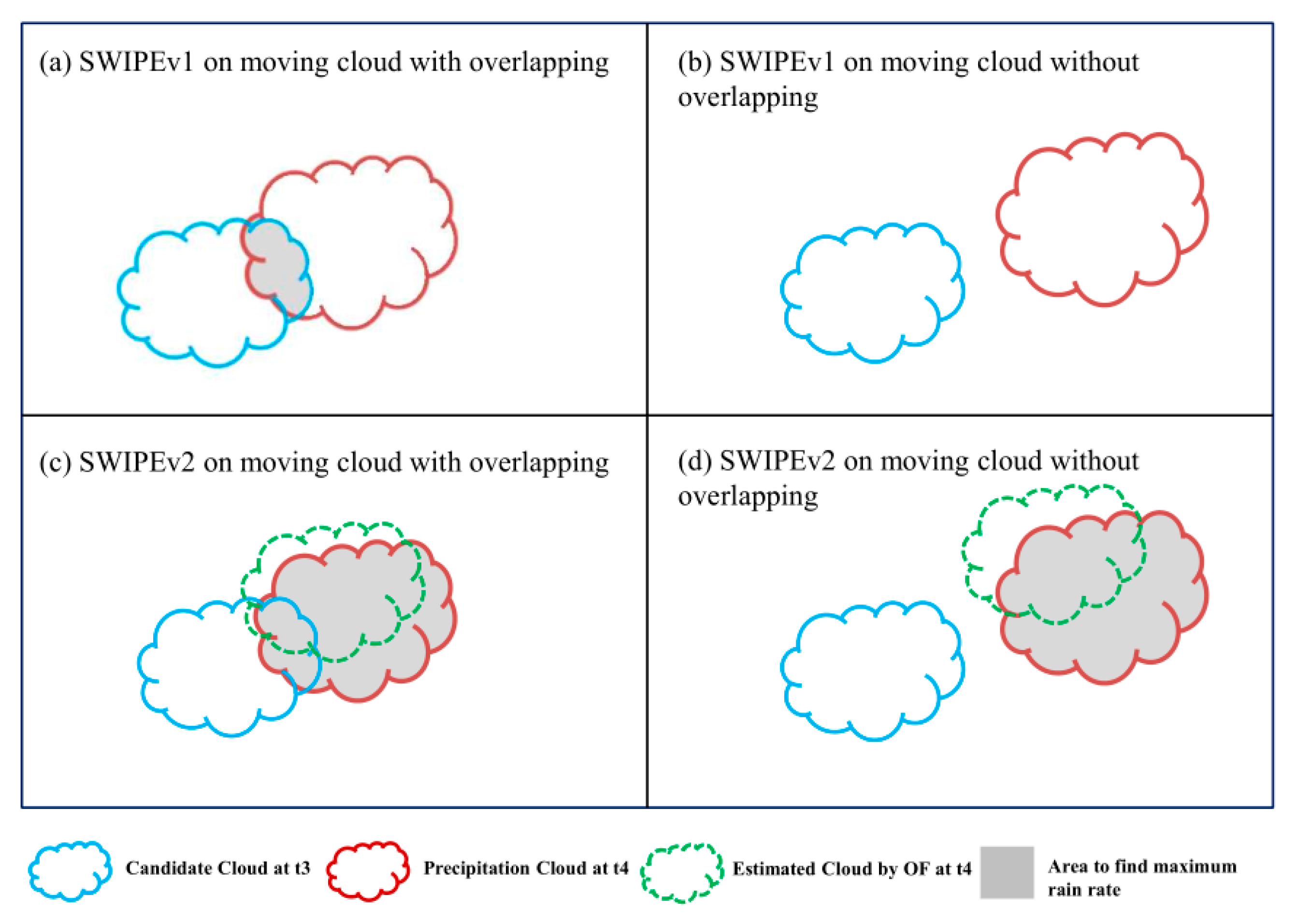
  • During the collocation process, the collocated rain rate for a case was derived from the maximum value within the cloud region. This cloud region was determined at the time (t3) when the cloud candidates were identified. The movement of the convective cloud during the time period between the candidate identification and collocated rain rate was not considered. This could result in uncertainties in intensity classification, especially for those clouds with a maximum rain rate outside of the original cloud domain. Collocation with the moved cloud candidates at the time of the rainfall analysis data would be more accurate and objective.
  • Only the precipitation data closest in time was considered when building the training dataset. AHI has a scan rate of 10 min for the region of interest, while the time interval of the precipitation analysis (GPM and CMORPH) is 30 min; therefore, the time between identifying candidate clouds and the precipitation analysis was between 10 and 30 min. If the storm is not mature at the precipitation analysis time, the rain rate used does not reflect the true storm intensity. Some convective clouds may need more time to develop and to fully demonstrate their intensities. Therefore, further tracking and collocation with multiple rain rate analyses for the whole lifetime of the storm is required, ensuring the true maximum storm intensity is successfully characterized.

3.2. Optimized Model Framework for ABI

As an enhancement to the existing methodology, not only was the RF-based training framework applied to the CONUS region using observations from ABI, but efforts were also made to solve the existing limitations of SWIPEv1 mentioned above. The ABI CONUS observations with a 5-min time interval were used for the identification and tracking procedure. The tracking procedure was based on the brightness temperature (BT) of the 10.3 μm channel (channel 13 of ABI). This channel is the ‘clean’ IR window channel, which is less sensitive to water vapor absorption than other IR window channels, and is most useful for monitoring cloud-top growth [31]. The threshold for monitoring was kept as two consecutive cooling rates exceeding −16 K/h, the same as was used by the authors in [16], but with a 5-min interval. The tracking was performed continuously, i.e., every 5 min. This was more frequent than the AHI 10-min window. As a result, the model had a better chance of capturing the initiation of local convection at a slightly earlier time (from 5 to 15 min earlier depending on the cooling situation). This improvement of 5 to 15 min in lead time is important for local severe storm nowcasting. [43,44].
Figure 1 shows an example of how the candidate clouds were tracked through area overlapping and identified through thresholds. Figure 1f shows that not all convective clouds were candidates. Clouds with cloud tops reaching the tropopause were not candidates because their cooling rates did not exceed the threshold. For example, the northeast–southwest convective cloud belt extending from Lake Superior to northern Illinois showed two convective cloud tops below 220 K, but the cooling rates for the two time steps were positive values, which indicated already developed convection rather than CI. Thus, the model targets CI.
A major enhancement for building the dataset was the consideration of cloud movement in the collocation of the precipitation data. This ensured the collocated maximum rain rate came from the whole domain of the same candidate cloud. See Section 3.1 (SWIPE model and existing issues) of this paper for an explanation of why enhanced cloud tracking is needed. Ideally, the tracking should be carried out continuously from the tracking time t3 to the CMORPH time at t4. The CMORPH time was specially designed to be 15 to 45 min after t3. This ensured the CMORPH time was not too close to t3 so that the nowcasting model had a meaningful and reasonable lead time, and was not too far away from t3 so that the area overlapping could be successful between t3 and t4. The relatively large time difference between t3 and t4 significantly increased the computational burden for tracking.
To overcome that burden, we used an estimation to project the movement. This estimation was carried out by introducing the classical dense optical flow (OF) algorithm [45] to predict the candidate cloud’s location at the time of CMORPH data from the consecutive images used in convective tracking. The algorithm detected the changes between two frames from all the pixels and calculated the motion vectors of each pixel from two dimensions, i.e., Fx, Fy. Then, the moving components of a candidate cloud were acquired from the averaged OFs of pixels that belong to the specific cloud. After that, a temporal extrapolation was performed to obtain the estimated range and predict the location of the candidate cloud at t4.
To find the actual location and domain of the candidate cloud at t4, the final area overlapping was applied between the predicted cloud and the actual ABI imagery at t4. Once the candidate cloud at t4 was identified, the maximum precipitation rate at t4 was found from the domain of the actual candidate cloud. Figure 2 shows a schematic of the collocation process with OF and additional area overlapping with ABI imagery at t4 included. This enhanced method can benefit the CI model with a more accurate spatial range of rainfall detection in training, and provide important information on the potential movement of clouds in real-time nowcasting applications. Figure 3 shows the comparison of flow charts of the tracking and collocation process in building the training dataset for the original SWIPEv1 and enhanced SWIPEv2.
However, the maximum rain rate does not necessarily happen at CMORPH data time t4. It could happen 30 min later (t5), or 1 h later (t6). Therefore, it is important to examine multiple time steps of the rain rate data for collocation to improve the classification of the intensity. This was carried out by applying the same collocation techniques (OF plus the area overlapping) from t4 to t5 and from t5 to t6 (the second and third CMORPH data time after identification). The maximum rain rate from all collocated CMORPH data corresponding to the same cloud candidate was considered the final value and criterion for intensity classification. It is worth noting that only when a cloud can be tracked and matched with a cloud candidate from the previous image can it be considered valid. Otherwise, the collocation process will stop at the previous CMORPH time and the result will be based on the valid results. In addition, the cloud-top BT from the ABI image of a latter CMORPH time should be no more than 3 K warmer compared to that of the former one. This ensures that the convective cloud should at least have developed or maintained a similar cloud top after the previous CMORPH time. If the cloud-top BT is substantially (3 K) warmer than that of a previous time, it indicates either the system is in the dissipating stage or is of a completely different system. In such cases the rainfall intensity at this time should not be considered as the basis for classification.
An added quality control step was performed on those cases for which the collocation process stopped before t6. This was carried out by labeling the cases whose lifetime minimum cloud-top BT was higher than 241 K (−32 °C) as class 0 (‘non-convective’), because those warm clouds should not be considered convective systems [7]. This procedure is essential because the goal of this work was to nowcast local convective initiation, while precipitation from stratiform clouds without convection that could possibly be tracked with cooling cloud tops should not trigger warnings. By introducing the OF algorithm and continuous tracking for precipitation, the collocated dataset for training could have an enhanced correlation between the predictors in pre-convection environments and their intensities. Note that there was no continuous tracking for precipitation after t6. That means the nowcasting model focuses on very short-term systems, i.e., within the next 1 h and 45 min, although the model could be applied to storms with lifetimes longer than that, as will be shown in Section 4. The limit of 1 h and 45 min is more than the average lifetime of 20–30 min for thunderstorms in northern Texas, Oklahoma and Kansas [44]. Only 6.9% of storms have a lifetime longer than 1 h. These enhancements in SWIPEv2 improved the quality of the collocation dataset, which in turn benefited the predictive model. For example, the application of in tracking the movements of cloud candidates resulted in 1071 additional severe samples compared to non-OF collocations, which indicates a labelling correction of around 5.0% of the severe samples. Compared with the collocation results from precipitation of the nearest time, there were 4816 more severe samples identified by the enhanced framework with continuous tracking, which is 22.4% of the severe class sample size. Statistical results show that there were 1523 non-severe cases that were mistakenly identified as severe due to the lack of quality control, which is likely associated with non-convective precipitation. With the enhanced tracking and collocation framework, the lead times between when a candidate was identified and when it was labelled by precipitation was in a range of 20 to 105 min. This is much longer than that of SWIPEv1, whose lead time for collocation is 10 to 30 min.

3.3. Convective Dataset

Seven continuous months of convective cases from the CONUS region (60°W~150°W, 10°N~50°N, from March to October 2018) were tracked using ABI 10.3 µm band BT measurements and collocated with the corresponding GFS NWP variables to build the dataset for training the CI model. Shown by Table 1 are the variables collocated from both datasets that are used as predictors of SWIPEv2. As there was no clear threshold in the US for a convective intensity definition based on precipitation rate, we adopted the classification thresholds of rainfall intensity defined by the American Meteorological Society (AMS) as the basic indicator for classification. The cases in this study were divided into three classes based on their maximum rain rates from CMORPH. The thresholds were as follows: (1) Candidates with a maximum rain rate no more than 2.5 mm/h were classified as weak or non-convective cases, (2) Candidates with a maximum rain rate between 2.5 mm/h and 7.6 mm/h were classified as moderate cases, (3) Candidates with a maximum rain rate more than 7.6 mm/h were classified as severe cases [46]. Both weak and moderate classes were considered non-severe.
Next, the samples were randomly split into two groups: a training group consisting of 80% of the overall samples to be fed into the RF framework to train the model, and a validation group using the remaining 20% set aside after the training process to be used for independent model evaluation. Further analysis on predicting skills of the enhanced algorithm was carried out using the validation dataset that was not included in the training process. In addition, the representativeness of the validation set was verified through a five-fold cross-validation ensuring that the impact from different separations on statistical performance was minor. Shown in Table 2 are the sample sizes for different groups and classes. Note that these sample sizes are for the convective candidates that were to be monitored and n via the RF model, rather than convective storm systems in synoptic definition.

4. Prediction Model

4.1. Random Forest Training

Inherited from the experience of SWIPEv1, the random forest (RF) algorithm, which is very useful for classification problems [47,48], was adopted as the machine learning framework for the enhanced SWIPEv2. For a detailed description of the RF algorithm, readers are referred to the classic paper on this method [42] and the brief introduction by coauthors of this article in the Appendix of the paper on SWIPEv1 [29]. Following the flowchart shown in Figure 3, the random forest (RF) classification model was developed with collocated ABI and GFS NWP variables serving as the predictors for each CI candidate. The corresponding intensity determined from the tracked maximum precipitation rate functions as the truth label. A random forest classifier trains a number of decision tree classifiers on different sub-samples using different predictors, and uses averaging to provide an ensembled result [42]. In this study, the training process was implemented using the free and efficient Scikit-learn toolkit [49]. It is worth noting that there was a significant imbalance among the sample sizes of each class. Overall, 94.3% of the candidate samples were weak or non-severe convective storms; this was significantly more than the percentage of moderately severe storms (3.0%) and severe storms (2.7%). Previous studies [50] have demonstrated the negative impact of unbalanced sample sizes among classes on the performance of machine learning classification models. In this study, models with original unbalanced sampling and balanced sampling were trained in parallel to compare the abilities of nowcasting under different sampling configurations. Three major hyperparameters, including the total number of decision trees (n_estimators), the maximum depth of the tree (max_depth) and the maximum number of predictors to consider when looking for the best split (max_features), were tuned iteratively to find the optimal model setting under each specific scenario. Shown in Table 3 are the different scenarios under which the training procedures were conducted, and their respective features shown after the training. For each scenario, the hyperparameters were exhaustively iterated within the following lists, [100, 200, 300, 400, 500, 1000] for parameter ‘n_estimators’, [10, 20, 30, 40, 50] for ‘max_depth’ and [5, 10, 20, 30, 40, ‘sqrt’, and ‘log2′] for ‘max_features’.
For each combination of hyperparameters, the out-of-box (OOB) score of the RF model was calculated to evaluate the generalization skills of the model using the out-of-bag samples within the training dataset that were randomly left out when building the decision trees [51]. In addition, the overall classification accuracy for each model was calculated on the independent validation dataset shown in Table 3. On top of the triple-group models from the previous version by Liu et al. [29], double-group classifications were accomplished by combining the moderate class and the weak/none class into one group, which was then classified against the severe class as a ‘severe against non-severe’ classification model. It is obvious from Table 3 that under all scenarios, the standard deviations (STDs) of the out-of-box (OOB) scores and overall accuracy values were very small compared to their respective mean values. This indicated that the fitting performance in this study was not sensitive to the combination of parameters, and the major difference came from the training framework and sampling approaches. Generally, the double-group models showed higher OOB scores and better overall accuracies compared with their triple-group counterparts, implying fewer classification errors and better stability in performance.
When comparing the results under the same classification framework, the unbalanced models showed better OOB scores and higher accuracy than the balanced models. However, this was most likely due to the extreme imbalance of the sample sizes in both the training and validation datasets. As previous studies have shown that ML models would be biased towards the largest class with poor performance for predicting the minority classes [50], and because the weak class covered over 94% of the total sample size, the results from this class would have misleading effects on the overall accuracy. For instance, the overall accuracy could be as high as 0.94 if all samples were blindly classified as ‘weak’. Since the focus here was on severe storms, the accuracy on these cases should be the key indicator of model performance, and the results have been further analyzed in Section 4.

4.2. Model Evaluation

Based on the discussions above, some indicators based on the confusion metrics were adopted to evaluate the model performances for certain classes, especially the severe class. Shown in Table 4 and Table 5 are an example of a contingency table for predictions and actual labels for a specific group, and the metrics calculated based on the confusion matrix to evaluate the model performances, respectively.
Shown in Table 6 are the performance metrics of different classes calculated using different models. Each model was optimized with regard to the hyperparameters to reach the best probability of detection (POD) score and maximize the prediction of the severe class. For fair comparisons, all the models with different configurations were validated against the same unbalanced testing dataset, which was similar to that in the real world. According to the statistics in Table 3, the variation in overall OOB score and accuracy was very tiny within each scenario, which means these selected models were representative of their respective scenarios, and showed the best accuracy for severe storms among the hyperparameter combinations.
Table 6 shows that the balanced models (Scenario 3CBA and 2CBA) performed better than the original models (Scenario 3CUB and 2CUB) in terms of the POD score of severe cases, at the expense of higher false alarm rates (FARs). As for the original models, despite the fact that they had better critical success index (CSI) scores for the severe class compared to their balanced counterparts, their POD values were below 0.40 which means they missed the majority of severe cases. This was mainly due to the imbalanced proportion of different classes in the training set (shown in Table 2) that led to biased performances towards the dominant class, or the weak/non-severe samples in this case.
Despite some false alarms, as the nowcasting model focused on providing warning signals in the pre-convection stage, we considered capturing as many severe convective samples as practical to be a higher priority. Considering the fact that the severe samples only made up approximately 2.7% of the total tracked candidates, as long as the model could distinguish the potentially severe cases from the vast majority of candidate storms in Section 3, it was possible to make corrections to reduce the false alarms with reference to subsequent radar echoes. In this way, the balanced models trained under Scenario-3CBA and Scenario-2CBA were preferred in this study. However, it is worth noting from Table 6 that both of the triple-group models showed poor skill for the moderate class, with either scarce detection or a very high number of false alarms. Since our focus was on severe convection, and model 3CBA showed the highest CSI score for the severe class while 2CBA showed the highest POD among the four, the capability of the two frameworks needed further evaluation.
In order to further investigate how these models performed for severe storms, we separated the tracked candidates in the validation dataset into three groups based on the area covered by the candidate cloud at the time of identification (t3 in Figure 3). The four selected models were then validated separately for each group to determine the nowcasting capability of the different models on targets with different sizes.
Shown in Figure 4a are the frequencies of occurrence for different sizes of non-severe and severe cases. While the ratio of non-severe to severe cases for those candidates with areas less than 1000 km2 was as high as 101.75, the number of non-severe cases was only approximately four times that of the severe cases for samples with areas over 5000 km2. The large-area group also had the most severe case occurrences among the three, consisting of approximately 45% of the total severe samples from the whole dataset, much more than for the small- and medium-area groups. That means large severe storms are more common. Since large severe storms are more likely to cause more damage than smaller ones due to their broader spatial coverage, it is important to ensure that the nowcasting tool is useful for large severe storms.
Figure 4b–d show the metric scores of POD, FAR and CSI for the severe classes for small storms with areas of no more than 1000 km2, medium storms with areas ranging between 1000 and 5000 km2, and large storms with areas over 5000 km2, respectively. Drawn from comparison among the three groups, each of the four models showed its best performance on the large group, with the highest POD and CSI among the groups and FAR significantly smaller than POD. This result indicates that the SWIPEv2 identification and tracking methodology showed more skill nowcasting severe storm systems with larger spatial scales regardless of the training configurations. This means the SWIPEv2 is particularly useful for large storms associated with more damage.
When comparing the models, the 2CBA model had the highest POD score of 0.99, indicating that almost all severe cases in this group could be successfully predicted. However, model 2CBA also had the largest FAR value of 0.63 among the four models, which meant a significant number of false alarms were given along with the correct signals, and that led to the lowest CSI score for 2CBA among the models. The other three models showed better CSI scores close to each other, with the highest score coming from model 3CUB. However, as large severe storms are more likely associated with damage compared to smaller ones, it is always necessary to capture as many potentially severe storm candidates as possible. Therefore, in spite of its higher FAR than the other two models with similar CSI scores, model 2CBA showing higher PODs may be regarded as the optimal model for this group. The results of 3CBA should also be considered to help with real-time nowcasting as it rarely missed a severe candidate covering a large area. Storms predicted by both models as severe will be warned as severe. If one model predicts a storm as severe while the other predicted it as non-severe, it will be warned as ‘potentially severe.’ Continuous monitoring using follow-up observations may help correct the false alarms.
In terms of the small-area group (Figure 4b) and medium-area group (Figure 4c), the POD scores for the imbalanced models, 3CUB and 2CUB, decreased drastically compared with the large-area group. While the drops in POD for 3CBA and 2CBA were not that significant, the FAR values were much larger compared to the large-area group. All four models showed the worst overall performance on severe samples with areas less than 1000 km2. In particular, the imbalanced models 3CUB and 2CUB showed almost no skill in predicting the severe cases in this group. This is partly because the spatial range of small cloud candidates less than 1000 km2, approximately 32 km × 32 km, was smaller than the spatial resolution of the GFS NWP gridded data, which was collocated in the predictors to provide the environmental background information. Without adequate information from the atmospheric background, it could be difficult to make an accurate prediction of the future severity and evolution of a convective cloud from only its BT spectra at the pre-convection stage. Refer to Section 4.4 for the relative importance of NWP in comparison to satellite data. Compared with larger systems, the motions of small cloud candidates are more difficult to track and accurately predict via the OF methodology, which adds to the uncertainties in the collocation of precipitation through area overlapping. For small and medium candidates, model 2CBA can only be relied on to capture the most severe cases, while the results of model 3CBA can be used to determine those severe samples that are less likely to be false alarms.
Further analysis of the results from models 3CBA and 2CBA shows that, out of the severe cases correctly predicted by model 3CBA, 100% of the large cases, 99.85% of the medium-sized cases and 98.69% of the small cases were also correctly predicted by 2CBA. Meanwhile, out of the false alarmed cases produced by 3CBA, 99.42% of the large cases, 99.21% of the medium-sized cases and 95.16% of the small cases were also among the false alarms from 2CBA. This reveals a high correlation between the prediction skills of models 3CBA and 2CBA on severe storms, with the former providing conservative prediction results with less severe warnings and fewer false alarms, and the latter giving more severe warnings with higher POD and higher FAR. Therefore, an ensembled framework was developed for potential real-time nowcasting by taking advantage of the benefits from both models through a two-level warning. If a cloud candidate was predicted as severe by both models, it was marked as ‘severe’; and if it was predicted as severe by only one model, it was marked as ‘potentially severe’. Shown in the bottom row of Table 6 is the statistical performance of the ensembled model on severe cases. When the two-level warnings were considered, the false alarm rate decreased significantly, while the POD of severe cases remained high. The other two models, 3CUB and 2CUB, were not used in the ensembled framework due to their overall low prediction skills.

4.3. Case Demonstration

The tracking and prediction model trained and validated with data from 2018 was tested on independent real cases in August 2019. Based on validation results from different scenarios, predictions were carried out as an ensemble classification model. The tracked candidates predicted as severe by both models 3CBA and 2CBA were marked as ‘severe,’ and those candidates predicted as ‘severe’ by only one (mostly from B2) of the two models were marked as ‘potentially severe’ indicating a possible severe storm, but this could also indicate a false alarm. The enhanced SWIPEv2 model could identify the candidates and give predictions with the same time interval of 5 min as ABI for the CONUS region, and the averaged time cost from reading in datasets to giving predictions was approximately two minutes. Once a warning signal was issued in real-time application, a follow-up tracking module continued tracking the cloud candidate until it could be identified from radar observations. This allowed forecasters to monitor the further development of those previous candidates that were predicted with severe storm potential when they were no longer identified as CIs due to development. As this follow-up module was purely tracking and designed only for real-time application, it has not been shown in this study. A typical storm event documented by the Storm Prediction Center (SPC, https://www.spc.noaa.gov/exper/archive/events, accessed on 7 August 2019) was tracked and predicted by the enhanced SWIPEv2 model in its pre-convection stage, and is illustrated in detail for demonstration purposes.
A pair of convective systems were identified successively by the enhanced SWIPEv2 system with an interval of 30 min, before developing and merging into a larger system and resulting in hail, strong winds and heavy rainfall in northeastern Wisconsin on 7 August 2019. The results are presented in Figure 5. The first severe warning prediction was issued at 1655 UTC, when the cloud-top BT was around 250 K with light rainfall under 2 mm/h. Another storm candidate to the west of the previous one was identified and predicted as severe at 1725 UTC. The two storms were independent of each other at this time and each had its own associated precipitation shown on the CMORPH plots.
The storm in the west then moved closer to the one in the east and started merging at 1800 UTC when the associated maximum precipitation rate first exceeded 7.6 mm/h from CMORPH. The two cloud candidates merged into a large cloud afterwards and showed a maximum precipitation rate over 12 mm/h at 1930 UTC. Hail and strong winds were also reported around this time. The convective system that produced hail and strong winds in Wisconsin was first captured by the enhanced SWIPEv2 model at 1655 UTC, over 2.5 h prior to its peak intensity. The smaller candidate that merged into it was also successfully identified prior to the merger and intensified convection.
Despite the success for this convection event, it should be noted that when clouds merge after they are identified and tracked as candidates, the severity is labeled according to the rainfall intensity of the merged clouds, and it is hard to distinguish the corresponding contribution from each cloud candidate under the current framework. This makes it possible that candidates with different characteristics at initiation times are collocated with the same intensity of convection as long as they merge into one big convective cloud. In particular, this is important to be aware of for cases when one small candidate not favorable for convection merges into a large convective cloud resulting in heavy rainfall, which might add uncertainties to the model when included in the training dataset. This might potentially reduce the skill of the model to correctly predict the severity of small-size candidates.

4.4. Relative Importance of Predictors

Despite the success for this convection event, the relative contribution of different predictors for the RF based classification model was evaluated through feature importance scores (IS) calculated using the Scikit-learn toolkit [49]. Shown in Table 7 are the top 10 ranked predictor variables with the highest ISs from ABI and NWP for the selected models 3CBA and 2CBA, respectively. The top ranked predictors for both models came from satellite observations from ABI, which made up the top five predictors for both 3CBA and 2CBA. Another consistency was that the maximum value of brightness temperature differences between channels 6.2 and 10.3 μm ranked at the top in both models. The BT differences between other water vapor (WV) channels (6.9 and 7.3 μm) and the window channel also had higher rankings in both models. This was in good agreement with previous studies in that the BT differences between a strong WV absorption band and a window band reflect the growth of cloud-top height relative to the tropopause, showing good correlations with potential convection, and can be used for nowcasting that convection [13,14,52]. This is also the reason why such BT differences have been used to identify deep convective clouds [53,54,55].
The differences between the two models were mainly in the feature importance of NWP variables. In terms of overall importance, ABI has a higher importance than the GFS NWP in both models, and it contributes more to model 3CBA than model 2CBA. While more predictors from the GFS NWP appeared in the top 25 rankings of model 2CBA, the top 2 ranked predictors from ABI observations outscored other predictors by large margins, and contributed over one-third of the total importance. This reveals that, compared to NWP variables from the GFS, the ABI predictors had much larger impacts for both models, and model 2CBA, with higher POD along with higher FAR, relies more on specific channel differences between the clean window channel and channels 6.2/9.6 μm, respectively.
It is worth noting that there are two ways that ABI may contribute to the storm nowcasting. Besides the direct use of ABI observations as predictors, ABI may provide useful information to the storm nowcasting indirectly through NWP predictors because the ABI clear sky radiances [56,57] and atmospheric motion vectors [58] have been assimilated into the GFS.

5. Summary

A storm nowcasting framework was developed for the CONUS region by combining high-resolution ABI observations with GFS forecasts as predictors, and by training through a random forest ML environment with a precipitation rate from CMORPH used as the truth label. This methodology was adapted from a previous framework named SWIPEv1 that used observations from AHI in combination with GFS forecasts to nowcast severe storms in East Asia. This study addressed some of the limitations of SWIPEv1 through optimizations in the following three aspects: (1) When searching for the truth precipitation rate associated with the tracked convective candidate, the movement of the target cloud is taken into account by introducing dense optical flow to estimate the location at the precipitation time, before an additional area overlapping procedure to confirm with the real observed BT; (2) Time periods to search for maximum rain rates are expanded to three consecutive CMORPH analysis, making the collocated labels more representative for candidates with longer periods of development and increased possibility to find maximum intensities; (3) Additional quality control procedures are also included to enhance the accuracy of convective storm tracking.
After the establishment of datasets tracked and collocated from March to October 2018, the enhanced SWIPEv2 model was trained through RF under different scenarios. Th results showed that severe cases with areas equal or larger than 5000 km2 were easier to nowcast over smaller samples. This is very important for nowcasting because severe storms with areas larger than 5000 km2 account for 45% of all severe storms, and large storms are likely associated with increased damage due to their larger spatial coverage. The ratio of different classes in the training was important. The balanced two-class model (1:1, both classes had similar sample sizes in the training), with moderate and weak classes combined as non-severe, showed the best POD for severe storms but with the highest FAR. The balanced three-class model (1:1:1) showed more balanced results of POD and FAR compared with the two-class model when dealing with samples with large areas. However, the balanced two-class model may be preferred to capture severe storms with smaller sizes as all other models showed a significant decrease in POD as the area of the candidate decreased. For candidates with an area less than 1000 km2, the imbalanced models (ratio of different classes not adjusted in the training) showed almost no skill.
The analysis of the relative importance of predictors revealed that the overall contribution from ABI observations was much higher than that from the GFS forecast. The top-ranked predictors were BT differences between channel 6.2 μm and channel 10.3 μm, followed by BT differences between the 10.3 μm channel and channels 6.9/7.3 μm and 9.6 μm. NWP predictors associated with atmospheric instabilities and moisture content also showed a relatively higher importance among the variables.
Application of the enhanced SWIPEv2 model was demonstrated with a typical storm event over CONUS from 2019. The model showed its capability to nowcast severe storms in the pre-convection stage by successfully issuing warnings approximately 1 h and 5 min prior to the occurrence of the first precipitation rate over 7.6 mm/h from CMORPH, and more than two hours before the storms reached their peaks of intensity.
There are still several limitations of this nowcasting model. For example, it only considers precipitation as an indicator of convective intensity, while there are storms that produce other forms of damage such as hail and severe winds but with little or no precipitation. It is also worth noting that this tracking algorithm based on cloud-top cooling rate was mainly focused on isolated storm candidates. For convection initiated over an existing larger cloud system, it would not be considered ‘local convective initiation’ and not applicable to the SWIPEv2 model. Hence, this model is likely to be more effective on precipitation-related local severe storms than other storms. Future work will include utilizing the published reports from SPC to add storms related to hail and strong winds, as well as tornadoes. Ground-based radar and surface observations can also be utilized complementary to precipitation observations in the training process as the truth indicator of convective storm intensity. The nowcasting model can also benefit from regional NWP forecasts with finer spatial and temporal resolutions, such as the high-resolution rapid refresh (HRRR) model, when the forecast vertical profiles can be accessed in near real time. This nowcasting model is less effective for severe storms with smaller sizes, i.e., smaller than 1000 km2. NWP data from GFS is not able to provide more accurate information regarding the local thermodynamic and dynamic information due to coarse spatial resolution. Hourly forecasts from HRRR with a spatial resolution of 3 km should be able to provide additional added value on the nowcasting.
While combining all of the available information from geostationary and polar orbiting satellites as well as NWP forecasts through data assimilation can be an effective approach for short-term forecasting [59], this study focused on the nowcasting (0~2 h) of local storms with meso-to-micro scales. Such storms are difficult to nowcast via NWP. To achieve this, real-time three-dimensional observations with high spatial and temporal resolutions are desired. As hyperspectral geostationary observations and derived products could provide valuable information on the pre-convection environment [60,61], resolutions are proven to have a significant impact on the capability of hyperspectral sounders in capturing the fine spatial variations of the atmosphere [62]. Geostationary hyperspectral infrared sounders with resolutions higher than ERA5, such as 12 km from on-orbit GIIRS on Fengyun-4B [63], 4 km from the to-be-launched IRS onboard MTG from EUMETSAT [64], and the planned geostationary extended observations (GeoXO) sounder (GXS) [65], should be expected to provide additional benefits to the nowcasting of local severe storms with small scales. In addition, geostationary hyperspectral infrared sounders have the potential to capture low-level pooling and mid-level drying of the atmosphere before ABI sees the cloud-top cooling. Soundings with such information, when incorporated into SWIPE, may further improve the lead time. This potential has not been discussed in this study as the focus was on nowcasting the intensity after the candidate storm was identified from ABI. Finally, it should be noted that radiances from high spatiotemporal geostationary hyperspectral infrared sounders can be used directly instead of soundings in the enhanced SWIPEv2 model when such data are available.

Author Contributions

Conceptualization, Z.M., Z.L. and J.L.; methodology, Z.M., Z.L. and M.M.; software, Z.M., M.M. and X.W.; validation, Z.M., Z.L. and J.L.; formal analysis, Z.M., Z.L. and M.M.; investigation, Z.M., Z.L., J.L. and M.M.; resources, Z.L., J.L., J.S.; data curation, Z.M.; writing—original draft preparation, Z.M.; writing—review and editing, Z.L., J.L., J.S., M.M., T.J.S. and L.C.; visualization, Z.M.; supervision, Z.L. and J.L.; project administration, T.J.S. and L.C.; funding acquisition, Z.L. All authors have read and agreed to the published version of the manuscript.

Funding

This work was supported in part by the NOAA Quantitative Observing System Assessment Program (QOSAP) nowcasting OSSE project under Grant NA20NES4320003.

Data Availability Statement

GOES-16 ABI radiance data were provided by the University of Wisconsin, Madison SSEC Data Center (https://www.ssec.wisc.edu/datacenter, accessed on 15 March 2022), GFS NWP data were obtained from NOAA NCEP (https://www.ncdc.noaa.gov/data-access/model-data/model-datasets/globalforcast-system-gfs, accessed on 17 February 2022) and CMORPH precipitation data were obtained from NOAA NCEI (https://www.ncei.noaa.gov/data/cmorph-high-resolution-global-precipitation-estimates/access/, accessed on 17 February 2022).

Acknowledgments

The authors would like to thank Frank Marks from AOML/NOAA for his comments on this study, and Leanne Avila from SSEC for her English proofreading. The views, opinions and findings contained in this report are those of the authors and should not be construed as an official NOAA or US government position, policy or decision.

Conflicts of Interest

The authors declare no conflict of interest.

References

  1. Johns, R.H.; Doswell, C.A., III. Severe Local Storms Forecasting. Weather Forecast. 1992, 7, 588–612. [Google Scholar] [CrossRef]
  2. Doswell, C.A. Severe Convective Storms—An Overview. In Severe Convective Storms; Springer: Boston, MA, USA, 2001; pp. 1–26. [Google Scholar]
  3. Browning, K.A.; Blyth, A.M.; Clark, P.A.; Corsmeier, U.; Morcrette, C.J.; Agnew, J.L.; Ballard, S.P.; Bamber, D.; Barthlott, C.; Bennett, L.J.; et al. The Convective Storm Initiation Project. Bull. Am. Meteorol. Soc. 2007, 88, 1939–1956. [Google Scholar] [CrossRef]
  4. Dixon, M.; Wiener, G. TITAN: Thunderstorm Identification, Tracking, Analysis, and Nowcasting—A Radar-Based Methodology. J. Atmos. Ocean. Technol. 1993, 10, 785–797. [Google Scholar] [CrossRef]
  5. Matyas, C.J.; Carleton, A.M. Surface Radar-Derived Convective Rainfall Associations with Midwest US Land Surface Conditions in Summer Seasons 1999 and 2000. Theor. Appl. Clim. 2010, 99, 315–330. [Google Scholar] [CrossRef]
  6. Roberts, R.D.; Rutledge, S. Nowcasting Storm Initiation and Growth Using GOES-8 and WSR-88D Data. Weather Forecast. 2003, 18, 23. [Google Scholar] [CrossRef]
  7. Maddox, R.A. Mesoscale Convective Complexes. Bull. Am. Meteorol. Soc. 1980, 61, 1374–1387. [Google Scholar] [CrossRef]
  8. Velasco, I.; Fritsch, J.M. Mesoscale Convective Complexes in the Americas. J. Geophys. Res. Atmos. 1987, 92, 9591–9613. [Google Scholar] [CrossRef]
  9. Mathon, V.; Laurent, H. Life Cycle of Sahelian Mesoscale Convective Cloud Systems. Q. J. R. Meteorol. Soc. 2001, 127, 377–406. [Google Scholar] [CrossRef]
  10. Vila, D.A.; Machado, L.A.T.; Laurent, H.; Velasco, I. Forecast and Tracking the Evolution of Cloud Clusters (ForTraCC) Using Satellite Infrared Imagery: Methodology and Validation. Weather Forecast. 2008, 23, 233–245. [Google Scholar] [CrossRef]
  11. Mecikalski, J.R.; Feltz, W.F.; Murray, J.J.; Johnson, D.B.; Bedka, K.M.; Bedka, S.T.; Wimmers, A.J.; Pavolonis, M.; Berendes, T.A.; Haggerty, J.; et al. Aviation Applications for Satellite-Based Observations of Cloud Properties, Convection Initiation, In-Flight Icing, Turbulence, and Volcanic Ash. Bull. Am. Meteorol. Soc. 2007, 88, 1589–1607. [Google Scholar] [CrossRef]
  12. Mosher, F. Detection of deep convection around the globe. In Proceedings of the Preprints, 10th Conference on Aviation, Range, and Aerospace Meteorology, American Meteorological Society, Portland, OR, USA, 13–16 May 2002; Volume 289, p. 292. [Google Scholar]
  13. Mecikalski, J.R.; Bedka, K.M. Forecasting Convective Initiation by Monitoring the Evolution of Moving Cumulus in Daytime GOES Imagery. Mon. Weather Rev. 2006, 134, 49–78. [Google Scholar] [CrossRef]
  14. Mecikalski, J.R.; Bedka, K.M.; Paech, S.J.; Litten, L.A. A Statistical Evaluation of GOES Cloud-Top Properties for Nowcasting Convective Initiation. Mon. Weather Rev. 2008, 136, 4899–4914. [Google Scholar] [CrossRef]
  15. Walker, J.R.; MacKenzie, W.M.; Mecikalski, J.R.; Jewett, C.P. An Enhanced Geostationary Satellite–Based Convective Initiation Algorithm for 0–2-h Nowcasting with Object Tracking. J. Appl. Meteorol. Climatol. 2012, 51, 1931–1949. [Google Scholar] [CrossRef]
  16. Sieglaff, J.M.; Cronce, L.M.; Feltz, W.F.; Bedka, K.M.; Pavolonis, M.J.; Heidinger, A.K. Nowcasting Convective Storm Initiation Using Satellite-Based Box-Averaged Cloud-Top Cooling and Cloud-Type Trends. J. Appl. Meteorol. Climatol. 2011, 50, 110–126. [Google Scholar] [CrossRef]
  17. McGovern, A.; Elmore, K.L.; Gagne, D.J.; Haupt, S.E.; Karstens, C.D.; Lagerquist, R.; Smith, T.; Williams, J.K. Using Artificial Intelligence to Improve Real-Time Decision-Making for High-Impact Weather. Bull. Am. Meteorol. Soc. 2017, 98, 2073–2090. [Google Scholar] [CrossRef]
  18. Boukabara, S.-A.; Krasnopolsky, V.; Stewart, J.Q.; Maddy, E.S.; Shahroudi, N.; Hoffman, R.N. Leveraging Modern Artificial Intelligence for Remote Sensing and NWP: Benefits and Challenges. Bull. Am. Meteor. Soc. 2019, 100, ES473–ES491. [Google Scholar] [CrossRef]
  19. Gagne, D.J.; McGovern, A.; Xue, M. Machine Learning Enhancement of Storm-Scale Ensemble Probabilistic Quantitative Precipitation Forecasts. Weather Forecast. 2014, 29, 1024–1043. [Google Scholar] [CrossRef]
  20. Mecikalski, J.R.; Williams, J.K.; Jewett, C.P.; Ahijevych, D.; LeRoy, A.; Walker, J.R. Probabilistic 0–1-h Convective Initiation Nowcasts That Combine Geostationary Satellite Observations and Numerical Weather Prediction Model Data. J. Appl. Meteorol. Climatol. 2015, 54, 1039–1059. [Google Scholar] [CrossRef]
  21. Han, D.; Lee, J.; Im, J.; Sim, S.; Lee, S.; Han, H. A Novel Framework of Detecting Convective Initiation Combining Automated Sampling, Machine Learning, and Repeated Model Tuning from Geostationary Satellite Data. Remote Sens. 2019, 11, 1454. [Google Scholar] [CrossRef]
  22. Sun, F.; Qin, D.; Min, M.; Li, B.; Wang, F. Convective Initiation Nowcasting Over China from Fengyun-4A Measurements Based on TV-L 1 Optical Flow and BP_Adaboost Neural Network Algorithms. IEEE J. Sel. Top. Appl. Earth Obs. Remote Sens. 2019, 12, 4284–4296. [Google Scholar] [CrossRef]
  23. Zhou, K.; Zheng, Y.; Li, B.; Dong, W.; Zhang, X. Forecasting Different Types of Convective Weather: A Deep Learning Approach. J. Meteorol. Res. 2019, 33, 797–809. [Google Scholar] [CrossRef]
  24. Horn, B.K.; Schunck, B.G. Determining Optical Flow. In Proceedings of the Techniques and Applications of Image Understanding. Int. Soc. Opt. Photonics 1981, 281, 319–331. [Google Scholar]
  25. Bowler, N.E.; Pierce, C.E.; Seed, A. Development of a Precipitation Nowcasting Algorithm Based upon Optical Flow Techniques. J. Hydrol. 2004, 288, 74–91. [Google Scholar] [CrossRef]
  26. Li, L.; He, Z.; Chen, S.; Mai, X.; Zhang, A.; Hu, B.; Li, Z.; Tong, X. Subpixel-Based Precipitation Nowcasting with the Pyramid Lucas–Kanade Optical Flow Technique. Atmosphere 2018, 9, 260. [Google Scholar] [CrossRef]
  27. Wu, Q.; Wang, H.-Q.; Lin, Y.-J.; Zhuang, Y.-Z.; Zhang, Y. Deriving AMVs from Geostationary Satellite Images Using Optical Flow Algorithm Based on Polynomial Expansion. J. Atmos. Ocean. Technol. 2016, 33, 1727–1747. [Google Scholar] [CrossRef]
  28. Cintineo, J.L.; Pavolonis, M.J.; Sieglaff, J.M.; Cronce, L.; Brunner, J. NOAA ProbSevere v2. 0—ProbHail, ProbWind, and ProbTor. Weather Forecast. 2020, 35, 1523–1543. [Google Scholar] [CrossRef]
  29. Liu, Z.; Min, M.; Li, J.; Sun, F.; Di, D.; Ai, Y.; Li, Z.; Qin, D.; Li, G.; Lin, Y.; et al. Local Severe Storm Tracking and Warning in Pre-Convection Stage from the New Generation Geostationary Weather Satellite Measurements. Remote Sens. 2019, 11, 383. [Google Scholar] [CrossRef]
  30. Schmit, T.J.; Griffith, P.; Gunshor, M.M.; Daniels, J.M.; Goodman, S.J.; Lebair, W.J. A Closer Look at the ABI on the GOES-R Series. Bull. Am. Meteor. Soc. 2017, 98, 681–698. [Google Scholar] [CrossRef]
  31. Schmit, T.J.; Lindstrom, S.S.; Gerth, J.J.; Gunshor, M.M. Applications of the 16 Spectral Bands on the Advanced Baseline Imager (ABI). J. Oper. Meteor. 2018, 6, 33–46. [Google Scholar] [CrossRef]
  32. Kanamitsu, M. Description of the NMC Global Data Assimilation and Forecast System. Weather Forecast. 1989, 4, 335–342. [Google Scholar] [CrossRef]
  33. Franzke, C.L.E.; Torelló i Sentelles, H. Risk of extreme high fatalities due to weather and climate hazards and its connection to large-scale climate variability. Clim. Chang. 2020, 162, 507–525. [Google Scholar] [CrossRef]
  34. Joyce, R.J.; Janowiak, J.E.; Arkin, P.A.; Xie, P. CMORPH: A Method That Produces Global Precipitation Estimates from Passive Microwave and Infrared Data at High Spatial and Temporal Resolution. J. Hydrometeorol. 2004, 5, 487–503. [Google Scholar] [CrossRef]
  35. Xie, P.; Yoo, S.-H.; Joyce, R.; Yarosh, Y. Bias-Corrected CMORPH: A 13-Year Analysis of High-Resolution Global Precipitation. Geophys. Res. Abstr. 2011, 13, EGU2011-1809. [Google Scholar]
  36. Xie, P.; Joyce, R.; Wu, S.; Yoo, S.-H.; Yarosh, Y.; Sun, F.; Lin, R. Reprocessed, Bias-Corrected CMORPH Global High-Resolution Precipitation Estimates from 1998. J. Hydrometeorol. 2017, 18, 1617–1641. [Google Scholar] [CrossRef]
  37. Habib, E.; Haile, A.T.; Tian, Y.; Joyce, R.J. Evaluation of the High-Resolution CMORPH Satellite Rainfall Product Using Dense Rain Gauge Observations and Radar-Based Estimates. J. Hydrometeorol. 2012, 13, 1784–1798. [Google Scholar] [CrossRef]
  38. Liu, J.; Xia, J.; She, D.; Li, L.; Wang, Q.; Zou, L. Evaluation of Six Satellite-Based Precipitation Products and Their Ability for Capturing Characteristics of Extreme Precipitation Events over a Climate Transition Area in China. Remote Sens. 2019, 11, 1477. [Google Scholar] [CrossRef]
  39. Mazzoleni, M.; Brandimarte, L.; Amaranto, A. Evaluating Precipitation Datasets for Large-Scale Distributed Hydrological Modelling. J. Hydrol. 2019, 578, 124076. [Google Scholar] [CrossRef]
  40. Su, J.; Lü, H.; Wang, J.; Sadeghi, A.M.; Zhu, Y. Evaluating the Applicability of Four Latest Satellite–Gauge Combined Precipitation Estimates for Extreme Precipitation and Streamflow Predictions over the Upper Yellow River Basins in China. Remote Sens. 2017, 9, 1176. [Google Scholar] [CrossRef]
  41. Morel, C.; Orain, F.; Senesi, S. Building upon SAF-NWC Products: Use of the Rapid Developing Thunderstorms (RDT) Product in Météo-France Nowcasting Tools. In Proceedings of the Meteorological Satellite Data Users’, Dublin, Ireland, 2–6 September 2002; pp. 248–255. [Google Scholar]
  42. Breiman, L. Random Forests. Mach. Learn. 2001, 45, 5–32. [Google Scholar] [CrossRef]
  43. Wagner, T.J.; Feltz, W.F.; Ackerman, S.A. The temporal evolution of convective indices in storm-producing environments. Weather Forecast. 2008, 23, 786–794. [Google Scholar] [CrossRef]
  44. Liu, W.; Li, X. Life Cycle Characteristics of Warm-Season Severe Thunderstorms in Central United States from 2010 to 2014. Climate 2016, 4, 45. [Google Scholar] [CrossRef]
  45. Farnebäck, G. Two-Frame Motion Estimation Based on Polynomial Expansion. In Image Analysis; Bigun, J., Gustavsson, T., Eds.; Lecture Notes in Computer Science; Springer: Berlin/Heidelberg, Germany, 2003; Volume 2749, pp. 363–370. ISBN 978-3-540-40601-3. [Google Scholar]
  46. AMS Glossary Glossary of Meteorology, American Meteorological Society. 2012. Available online: https://glossary.ametsoc.org/wiki/Rain (accessed on 17 February 2022).
  47. Li, Z.; Ma, Z.; Wang, P.; Lim, A.H.; Li, J.; Jung, J.A.; Schmit, T.J.; Huang, H.-L. An Objective Quality Control of Surface Contamination Observations for ABI Water Vapor Radiance Assimilation. J. Geophys. Res. Atmos. 2022, 127, e2021JD036061. [Google Scholar] [CrossRef]
  48. Min, M.; Bai, C.; Guo, J.; Sun, F.; Liu, C.; Wang, F.; Xu, H.; Tang, S.; Li, B.; Di, D.; et al. Estimating Summertime Precipitation from Himawari-8 and Global Forecast System Based on Machine Learning. IEEE Trans. Geosci. Remote Sens. 2019, 57, 2557–2570. [Google Scholar] [CrossRef]
  49. Pedregosa, F.; Varoquaux, G.; Gramfort, A.; Michel, V.; Thirion, B.; Grisel, O.; Blondel, M.; Prettenhofer, P.; Weiss, R.; Dubourg, V.; et al. Scikit-Learn: Machine Learning in Python. J. Mach. Learn. Res. 2011, 12, 2825–2830. [Google Scholar]
  50. Sun, Y.; Wong, A.K.; Kamel, M.S. Classification of Imbalanced Data: A Review. Int. J. Pattern Recognit. Artif. Intell. 2009, 23, 687–719. [Google Scholar] [CrossRef]
  51. Hastie, T.; Tibshirani, R.; Friedman, J. Elements of Statistical Learning, 2nd ed.; Springer: New York, NY, USA, 2009. [Google Scholar]
  52. Schmetz, J.; Tjemkes, S.; Gube, M.; Van de Berg, L. Monitoring Deep Convection and Convective Overshooting with METEOSAT. Adv. Space Res. 1997, 19, 433–441. [Google Scholar] [CrossRef]
  53. Ai, Y.; Li, J.; Shi, W.; Schmit, T.J.; Cao, C.; Li, W. Deep Convective Cloud Characterizations from Both Broadband Imager and Hyperspectral Infrared Sounder Measurements. J. Geophys. Res. Atmos. 2017, 122, 1700–1712. [Google Scholar] [CrossRef]
  54. Gong, X.; Li, Z.; Li, J.; Moeller, C.; Wang, W. Monitoring the VIIRS Sensor Data Records reflective solar band calibrations using DCC with collocated CrIS measurements. J. Geophys. Res. Atmos. 2019, 124, 8688–8706. [Google Scholar] [CrossRef]
  55. Aumann, H.H.; Desouza-Machado, S.G.; Behrangi, A. Deep Convective Clouds at the Tropopause. Atmos. Chem. Phys. 2011, 11, 1167–1176. [Google Scholar] [CrossRef]
  56. Liu, H.; Collard, A.; Derber, J.C.; Jung, J.A. Evaluation of GOES-16 clear-sky radiance (CSR) data and preliminary assimilation results at NCEP. In Proceedings of the 2019 Joint Satellite Conference, Boston, MA, USA, 30 September–4 October 2019. [Google Scholar]
  57. Liu, H.; Collard, A.; Derber, J.C.; Jung, J.A. Clear-Sky Radiance (CSR) Assimilation from Geostationary Infrared Imagers at NCEP. In Proceedings of the International TOVS Study Conference XXII, Saint-Sauveur, QC, Canada, 31 October–6 November 2019. [Google Scholar]
  58. Genkova, I.; Thomas, C.; Kleist, D.; Daniels, J.; Apodaka, K.; Santek, D.; Cucurull, L. Winds Development and Use in the NCEP GFS Data Assimilation System. In Proceedings of the International Winds Workshops 15 (IWW15), Virtual, 12–16 April 2021. [Google Scholar]
  59. Smith, W.; Zhang, Q.; Shao, M.; Weisz, E. Improved Severe Weather Forecasts Using LEO and GEO Satellite Soundings. J. Atmos. Ocean. Technol. 2020, 37, 1203–1218. [Google Scholar] [CrossRef]
  60. Li, J.; Liu, C.-Y.; Zhang, P.; Schmit, T.J. Applications of Full Spatial Resolution Space-Based Advanced Infrared Soundings in the Preconvection Environment. Weather Forecast. 2012, 27, 515–524. [Google Scholar] [CrossRef]
  61. Li, J.; Li, J.; Otkin, J.; Schmit, T.J.; Liu, C.-Y. Warning Information in a Preconvection Environment from the Geostationary Advanced Infrared Sounding System—A Simulation Study Using the IHOP Case. J. Appl. Meteorol. Climatol. 2011, 50, 776–783. [Google Scholar] [CrossRef]
  62. Di, D.; Li, J.; Li, Z.; Li, J.; Schmit, T.J.; Menzel, W.P. Can Current Hyperspectral Infrared Sounders Capture the Small Scale Atmospheric Water Vapor Spatial Variations? Geophys. Res. Lett. 2021, 48, e2021GL095825. [Google Scholar] [CrossRef]
  63. Yang, J.; Zhang, Z.; Wei, C.; Lu, F.; Guo, Q. Introducing the New Generation of Chinese Geostationary Weather Satellites, Fengyun-4. Bull. Am. Meteorol. Soc. 2017, 98, 1637–1658. [Google Scholar] [CrossRef]
  64. Holmlund, K.; Grandell, J.; Schmetz, J.; Stuhlmann, R.; Bojkov, B.; Munro, R.; Lekouara, M.; Coppens, D.; Viticchie, B.; August, T.; et al. Meteosat Third Generation (MTG): Continuation and Innovation of Observations from Geostationary Orbit. Bull. Am. Meteorol. Soc. 2021, 102, E990–E1015. [Google Scholar] [CrossRef]
  65. Adkins, J.; Alsheimer, F.; Ardanuy, P.; Boukabara, S.; Casey, S.; Coakley, M.; Conran, J.; Cucurull, L.; Daniels, J.; Ditchek, S.D.; et al. Geostationary Extended Observations (GeoXO) Hyperspectral InfraRed Sounder Value Assessment Report; NOAA/NESDIS Technical Report; National Oceanic and Atmospheric Administration (NOAA): Washington, DC, USA, 2021; 103p. [Google Scholar] [CrossRef]
Figure 1. Tracked convective storm candidates at 1940 UTC on 07/01/2018 over CONUS. Subplots are (ac) the three consecutive brightness temperature (unit: K) imagery of band 10.3 μm from ABI, (d,e) the maximum cooling rates (unit: K/h) calculated from tracked cloud candidates that exceeded −16 K/h, and (f) the identified potential convective candidates (masked by orange) to be monitored and nowcasted through the RF framework.
Remotesensing 15 02672 g001
Figure 2. Schematics of the application of optical flow and area overlapping in collocating precipitation data for fast moving cloud candidates. For a moving cloud that has some overlap with its original area at the time of identification, (a) the SWIPEv1 [29] searches for the maximum rain rate within the overlapped area, while (c) the enhanced SWIPEv2 is able to locate the whole area of the precipitation cloud through application of area overlapping with actual ABI imagery at t4 in the collocation process. For a moving cloud that does not have any overlapped area with its original area, (b) SWIPEv1 fails to find the corresponding rain rate, while (d) the enhanced SWIPEv2 is able to collocate the ABI image at t4 with an estimated cloud area provide by OF, and successfully find the whole area of the target precipitation cloud.
Remotesensing 15 02672 g002
Figure 3. The flowchart of the tracking and collocation framework of (a) SWIPEv1; and (b) SWIPEv2 to build the training dataset. Here, t1, t2 and t3 are times for (a) AHI; (b) ABI CONUS images with a time interval of (a) 10 min; (b) 5 min. In addition, t4, t5 and t6 are times for CMORPH precipitation data with a time interval of 30 min. Note that the continuous tracking for CMORPH precipitation at t5 and t6 enhances the chance to capture the true storm intensity based on the precipitation rate.
Remotesensing 15 02672 g003
Figure 4. (a) Sample sizes of non-severe and severe cases for small-area group (areas smaller than 1000 km2), medium-area group (areas in the range of 1000 to 5000 km2) and large-area group (areas no less than 5000 km2) in the validation dataset. POD, FAR and CSI scores for the severe cases with (b) small-area group, (c) medium-area group and (d) large-area group, respectively. Refer to Table 3 for the definition of the four scenarios.
Remotesensing 15 02672 g004
Figure 5. Two convective cloud candidates that merged into a severe convective storm case tracked by the enhanced SWIPEv2 model on 7 August 2019 in Wisconsin. The first row shows the greyscale BT of ABI’s 10.3 μm channel, overlaid with the results predicted by the enhanced SWIPEv2 model with ‘severe’ indicating unanimous classification decisions of severe from both models 3CBA and 2CBA, while ‘potential’ indicates split decisions from the two models with severe predicted by only one of them. The second row shows the colored BT(K) from ABI’s 10.3 μm channel. The third row shows the precipitation rate (mm/h) at the given times from CMORPH, with red circles marking the precipitation associated with the tracked storm system.
Remotesensing 15 02672 g005
Table 1. Predictor variables collocated for random forest training and prediction in the nowcasting model.
Data
Source
Variable 1Feature
ABI
CONUS
Maximum cooling rate (R1 and R2)Cloud-top cooling rate
AreaCandidate size
BT10.3Window channel brightness temperature
BT difference (3.9–10.3)Channel difference in brightness temperature
BT difference (6.2–10.3)
BT difference (6.9–10.3)
BT difference (7.3–10.3)
BT difference (8.4–10.3)
BT difference (9.6–10.3)
BT difference (11.2–10.3)
BT difference (12.3–10.3)
BT difference (13.3–10.3)
BT difference (3.9–7.3)
BT difference (3.9–11.2)
BT difference (8.4–11.2)
BT difference (11.2–12.3)
GFS
NWP
T (temperature)Basic profiles on pressure levels between 500 and 925 hPa
MR (Water vapor mixing ratio)
DIV (divergence)Characteristics of low-level atmosphere on 850 and 925 hPa
θ s e (pseudo-equivalent potential temperature)
DIV10 (divergence at 10 m above surface)Surface and near-surface information
Tsur (surface temperature)
PV (potential vorticity)PV on isentropic surface θ = 320 K
K-indexGeneral information of atmospheric instabilities and moisture
CAPE (convection available potential energy)
LI (lifted index)
CIN (convective inhibition)
EBS (effective bulk shear)
TPW (total precipitable water)
1 The maximum, minimum and mean values of each predictor variable in the domain of the candidate cloud (except maximum cooling rates and area coverage that are used directly) are used as inputs of the RF model.
Table 2. Sample sizes for convective candidates tracked in conus during March to October 2018.
DatasetWeak/NoneModerateSevereTotal
Training605,22319,20917,257641,689
Validation151,27448874262160,423
Overall756,49724,09621,519802,112
Table 3. The classification and sampling methodologies for different scenarios, and the mean value and standard deviations (in parentheses) of their respective OOB scores and overall accuracy compared to the validation dataset.
Scenario 1ClassificationSampling 2OOB Score 3Validation
Accuracy 4
3CUBTripleOriginal0.951 (0.0003)0.951 (0.0002)
3CBATripleBalanced0.663 (0.0053)0.794 (0.0022)
2CUBDoubleOriginal0.978 (0.0001)0.979 (0.0001)
2CBADoubleBalanced0.876 (0.0016)0.867 (0.0016)
1 A scenario named ‘3C’ used three classes (weak, moderate, and severe), while ‘2C’ represents two classes (non-severe and severe). UB here denotes original or unbalanced sampling, while BA represents balanced sampling. 2 The balanced sampling means all classes in the training had a similar sample size. 3 OOB score is the evaluation provided in the training process. For details, readers are referred to [51]. 4 The validation accuracy is the independent evaluation after the training using the independent validation dataset.
Table 4. Example of a contingency table for predictions and actual labels of a specific class in a classification task.
Observation
TrueFalse
PredictionTrueAC
FalseBD
Table 5. The metrics used to evaluate the performance of the random forest classification model on a specific class.
MetricFull NameFormulaRangeOptimal
PODProbability of DetectionA/(A + B)[0, 1]1
FARFalse Alarm RateC/(A + C)[0, 1]0
CSICritical Success IndexA/(A + B + C)[0, 1]1
Table 6. Statistics on the performance metrics of the storm nowcasting classification model trained and optimized under different scenarios. See Table 3 for the definition of each scenario.
ScenarioClassPODFARCSI
3CUBWeak/None0.990.040.95
Moderate0.030.550.03
Severe0.390.350.32
3CBAWeak/None0.810.010.80
Moderate0.580.900.09
Severe0.630.660.28
2CUBNon-Severe0.990.020.98
Severe0.310.250.28
2CBANon-Severe0.870.010.87
Severe0.900.840.15
Ensembled for Severe (3CBA + 2CBA)Severe0.900.580.40
Table 7. Importance scores of the top 10 ranked predictor variables 1 of RF models 3CBA (n_estimators = 1000, max_depth = 50, max_features = 5) and 2CBA (n_estimators = 500, max_depth = 30, max_features = 40). The total scores were calculated by summing the scores of all variables (not limited to the top 10 variables shown in the table) under the category.
ModelData SourceVariable ScoreRankingVariable ScoreRankingTotal Score
from the Source
3CBAABIdBT (6.2–10.3) max = 0.03461dBT (13.3–10.3) max = 0.028560.610
dBT (7.3–10.3) max = 0.03272BT (10.3) mean = 0.02107
dBT (6.9–10.3) max = 0.03193Area = 0.01759
dBT (9.6–10.3) max = 0.03094dBT (11.2–12.3) min = 0.017410
BT (10.3) min = 0.02925dBT (7.3–10.3) mean = 0.017011
GFS NWPK-index max = 0.01788DIV (925) min = 0.0128250.390
MR (850) max = 0.015615LI min = 0.010928
DIV (10m) min = 0.015018CIN max = 0.010731
Ɵse (850) max = 0.013123TPW max = 0.010434
K-index mean = 0.012924Ɵse (850) mean = 0.010436
2CBAABIdBT (6.2–10.3) max = 0.18041dBT (6.9–10.3) max = 0.029170.721
dBT (9.6–10.3) max = 0.17062Cooling rate (R2) = 0.009512
dBT (7.3–10.3) max = 0.06543dBT (3.9–11.2) max = 0.008813
BT (10.3) min = 0.06074Area = 0.007715
dBT (13.3–10.3) max = 0.03155dBT (11.2–12.3) min = 0.007117
GFS NWPƟse (850) max = 0.03146TPW max = 0.0080140.279
K-index max = 0.02218DIV (925) min = 0.007316
MR (850) max = 0.01979DIV (10m) mean = 0.006918
DIV (10m) min = 0.016610LI min = 0.006820
CIN max = 0.012411K-index mean = 0.006821
1 Variable names with ‘dBT (a–b)’ represent the difference in brightness temperatures between channels with wavelengths centering at a and b; numbers shown in brackets following NWP variables represent the pressure level of the variable; and ‘min, max, mean’ represent the minimum, maximum and mean values of the variables within the spatial region of the cloud candidate.
Disclaimer/Publisher’s Note: The statements, opinions and data contained in all publications are solely those of the individual author(s) and contributor(s) and not of MDPI and/or the editor(s). MDPI and/or the editor(s) disclaim responsibility for any injury to people or property resulting from any ideas, methods, instructions or products referred to in the content.

