Article

An Efficient Cloud Classification Method Based on a Densely Connected Hybrid Convolutional Network for FY-4A

1
College of Astronautics, Nanjing University of Aeronautics and Astronautics, Nanjing 210016, China
2
State Key Laboratory of Geo-Information Engineering, Xi’an 710054, China
3
Beijing Institute of Applied Meteorology, Beijing 100029, China
4
Space Optoelectronic Measurement & Perception Laboratory of BICE, Beijing 100094, China
*
Author to whom correspondence should be addressed.
Remote Sens. 2023, 15(10), 2673; https://doi.org/10.3390/rs15102673
Submission received: 22 February 2023 / Revised: 3 May 2023 / Accepted: 19 May 2023 / Published: 21 May 2023
(This article belongs to the Special Issue Computer Vision and Image Processing in Remote Sensing)

Abstract

:
Understanding atmospheric motions and projecting climate changes depends significantly on cloud types, i.e., different cloud types correspond to different atmospheric conditions, and accurate cloud classification can help forecasts and meteorology-related studies to be more effectively directed. However, accurate classification of clouds is challenging and often requires certain manual involvement due to the complex cloud forms and dispersion. To address this challenge, this paper proposes an improved cloud classification method based on a densely connected hybrid convolutional network. A dense connection mechanism is applied to hybrid three-dimensional convolutional neural network (3D-CNN) and two-dimensional convolutional neural network (2D-CNN) architectures to use the feature information of the spatial and spectral channels of the FY-4A satellite fully. By using the proposed network, cloud categorization solutions with a high temporal resolution, extensive coverage, and high accuracy can be obtained without the need for any human intervention. The proposed network is verified using tests, and the results show that it can perform real-time classification tasks for seven different types of clouds and clear skies in the Chinese region. For the CloudSat 2B-CLDCLASS product as a test target, the proposed network can achieve an overall accuracy of 95.2% and a recall of more of than 82.9% for all types of samples, outperforming the other deep-learning-based techniques.

1. Introduction

In the field of atmospheric and meteorological systems, cloud research has become essential. Clouds have a significant impact on the global atmospheric radiation balance as they reflect short-wave radiation and absorb and emit long-wave radiation, which in turn affects the Earth’s temperature [1,2]. An accurate and automated cloud classification has been used in many climatic, hydrological, and atmospheric applications. The diversity of cloud types is reflected in the structural patterns observed in clouds, and cloud types have a profound influence on the radiative effects of the Earth’s surface–atmosphere system [3,4]. Furthermore, geosynchronous meteorological satellite radiation scanners have become widely used meteorological observation tools, particularly due to the narrow observation range of polar-orbiting satellites and lengthy gaps between observations in the same region. Moreover, their ability to provide all-weather continuous large-scale observation is crucial for the continuous monitoring of cloud changes [5]. Therefore, developing a fast, precise, and autonomous cloud classification approach based on satellite data is essential [6].
According to the 2017 updated guidelines for cloud observation from the Earth’s surface published by the World Meteorological Organization (WMO) [
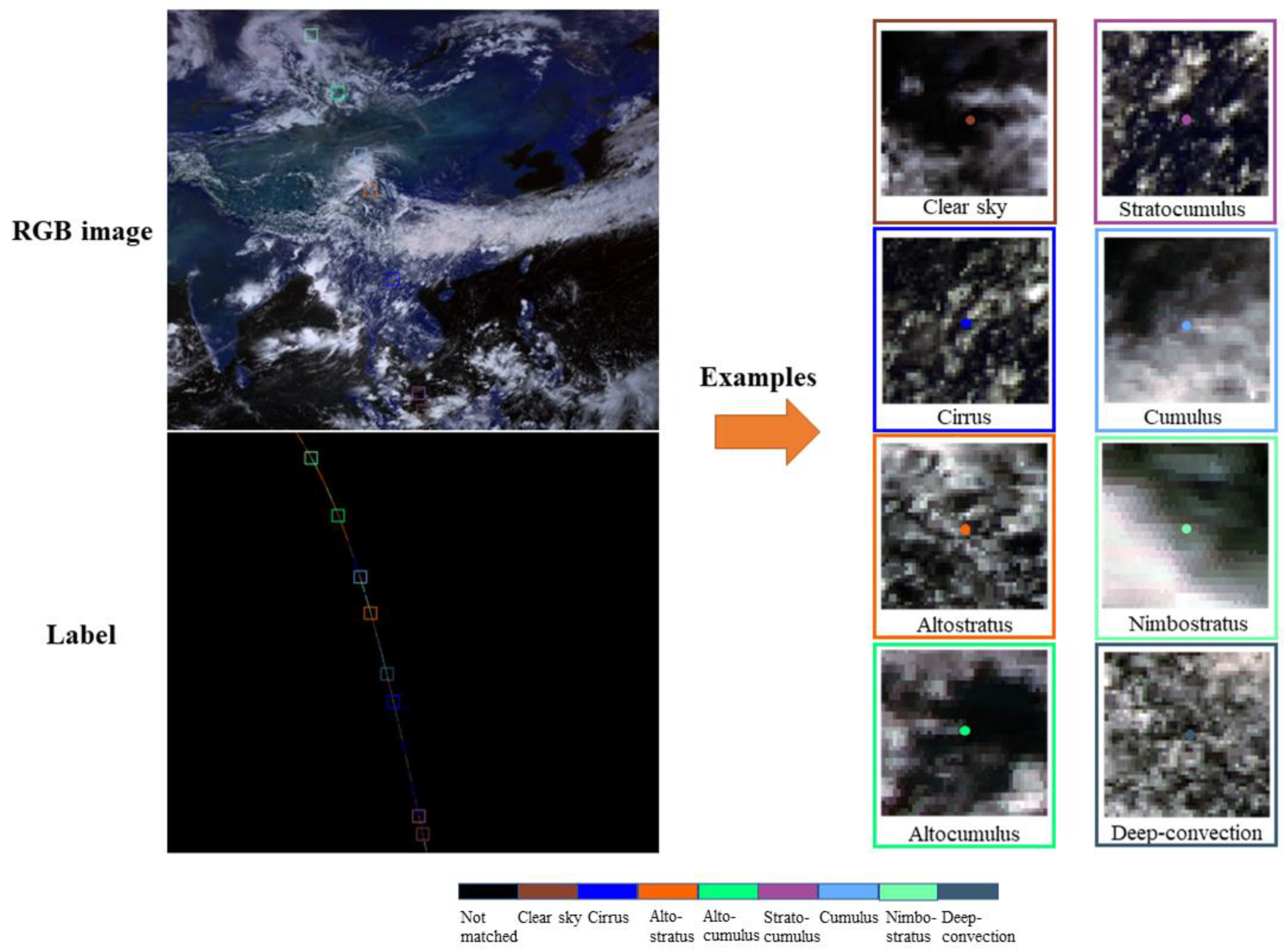
7], clouds can be grouped into three main categories, including low, middle, and high clouds, and into ten genera, such as cumulonimbus (Cb), cumulus (Cu), stratocumulus (Sc), stratus (St), nimbostratus (Ns), altocumulus (Ac), and altostratus (As). However, the accuracy of classification depends on an observer’s expertise and requires them to collaborate and rely on their professional knowledge to identify the correct cloud types based on macrostructure characteristics. Due to the subjective nature of manual classification, the classification results can be impacted. Research on cloud identification and categorization using satellite data has improved alongside advancements in satellite observation technologies [8,9]. The International Satellite Cloud Climate Project (ISCCP) has developed the standard for cloud classification based on satellite and ground data. Cloud types can be divided into nine categories based on cloud top pressure and cloud optical thickness [10,11]. Powerful satellites such as CloudSat, Cloud-Aerosol Lidar, and Infrared Pathfinder Satellite Observations (CALIPSO) can characterize three-dimensional (latitude, longitude, and altitude) cloud structures [12,13]. The cloud profiling radar (CPR) on CloudSat and the Cloud–Aerosol Lidar with Orthogonal Polarization (CALIOP) on CALIPSO can detect cloud particles at various altitudes, providing a vertical overlap structure for cloud layers [14,15]. CloudSat’s and CALIPSO’s cloud products have been extensively updated for over a decade and have frequently been used as benchmarks for validation and comparison purposes due to their widely recognized high quality [16,17]. However, limited coverage by polar-orbiting satellites in the same area and long intervals between observations make it challenging to observe daily cloud variability. Remote sensing investigations benefit from the superior temporal resolution and wider coverage of geostationary meteorological satellites. Bankert et al. analyzed and compared the explicit and implicit physical algorithm results for cloud type classification using GOES (Geosynchronous Orbiting Environmental Satellite) data [18]. The Japanese Aerospace Exploration Agency (JAXA) created a cloud classification system based on the ISCCP method for the Himawari-8 geosynchronous satellite, which is highly consistent with MODIS data [19,20]. The National Satellite Center of the China Meteorological Administration divides the FY-4A satellite’s cloud classification scheme into six categories: water, cold water, mixed, ice, cirrus, and overlap. However, the CLT’s cloud classification products contain fewer cloud types, and therefore an effective classification algorithm based on the ISCCP cloud classification scheme is urgently required.
Currently, there exist four fundamental cloud categorization techniques, namely, threshold approaches, split-window methods, texture-based methods, and statistical methods. The most popular cloud classification techniques, such as the split-window and threshold approaches, use data on reflectance, bright temperature, brilliant temperature difference, and sub-bedding type to identify the cloud type [21,22]. Nevertheless, these approaches may face failure in certain circumstances due to the intricacy of cloud systems, such as solar flare zones and high-latitude deserts, where fluctuations in brightness temperature differences can cause misinterpretations [23]. Since these approaches consume much information by employing all available bands, traditional mathematical and statistical methods, such as clustering and histogram methods, could be preferable to the threshold methods for cloud classification and detection [24,25]. However, applying them to individual clusters with significant overlap can be challenging. Furthermore, texture-based approaches have been evolved to determine the structure of various cloud types, but they fail to exploit long-term continuous observational data [26,27]. Additionally, K-means and support vector machine (SVM) approaches have been utilized for cloud classification tasks as a result of technological advancements, and they have obtained remarkable classification outputs [28,29]. However, the classification process neglects the cloud’s integrity, which impacts the classification outcome.
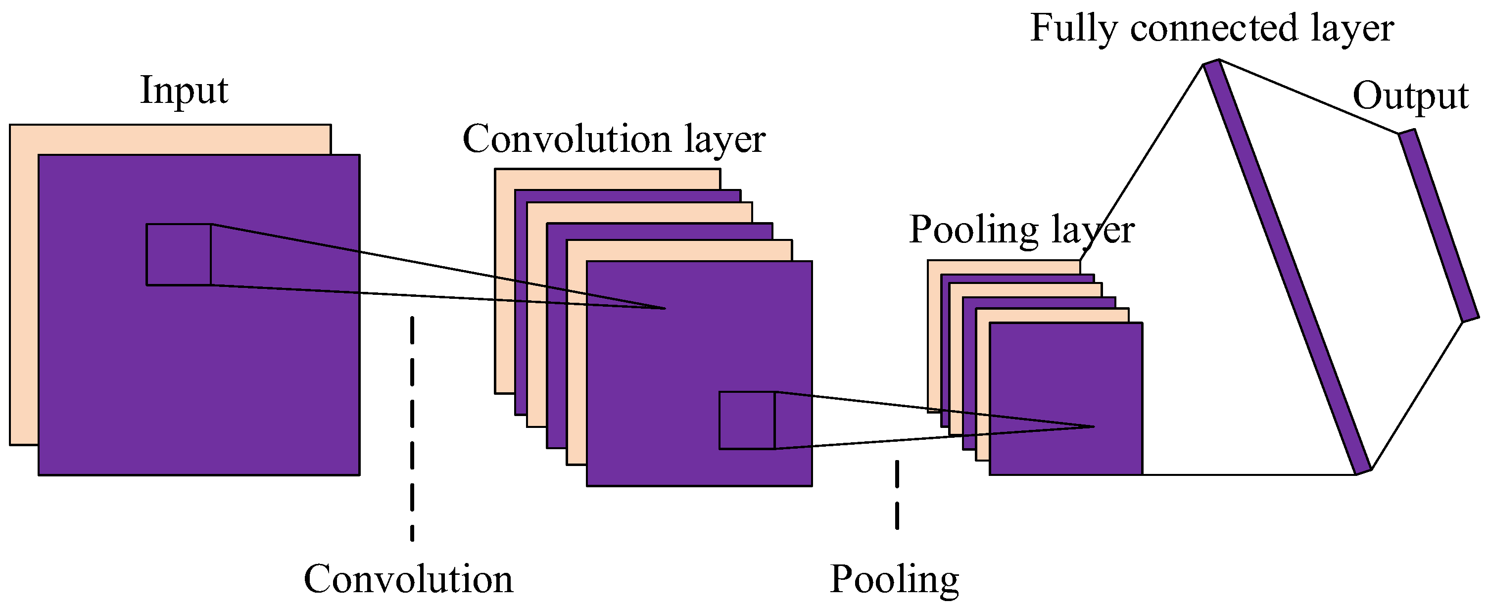
Many high-performance image-processing-based techniques have emerged, enabling the handling of massive amounts of data to become simpler and more effective. This development has significantly accelerated the advancement of deep learning. Furthermore, deep learning-based techniques have improved the accuracy and efficiency of cloud categorization tasks significantly. Artificial neural networks (ANNs) and convolutional neural networks (CNNs) have played vital roles in cloud classification techniques. Taravat et al. [30] achieved remarkable classification results by employing sky camera data and ANNs in their investigation of automatic cloud classification methods. Furthermore, Liu et al. [31] employed ANN models to classify FY-2C (Fengyun-2C) satellite photos and compared their results with those obtained using principal component analysis (PCA) and support vector machine (SVM). It should be noted that only the information within the current pixel can be considered in the above-mentioned ANN approaches. Zhang et al. [31] applied CNN models to recognize and categorize clouds in ground-based image data. The CNN models employ convolution to gather feature information in an image’s spatial domain, but they neglect both spectral channel dimension information and pixel-by-pixel cloud categorization. Jiang et al. [32] proposed an improved network based on U-Net and attained excellent cloud classification results on FY-4A (Fengyun-4A) data. Nevertheless, there are still some deficiencies, including poor network classification performance due to the dispersed and fragmented cloud morphology of the Ci, Ac, and other types, and confusion caused by the similar morphologies of Cu, Sc, and other clouds. Hence, there is still room for further improvement in this field.
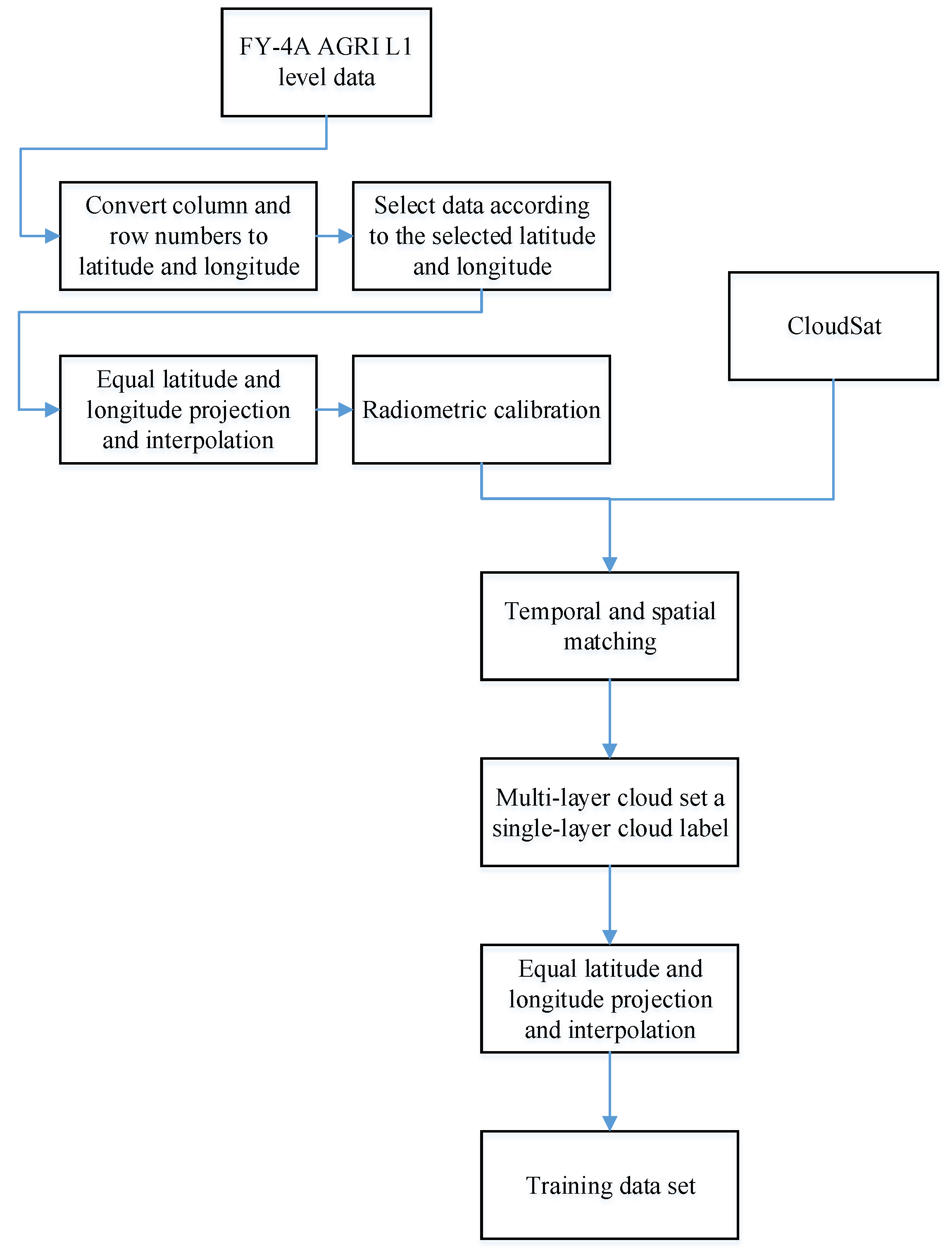
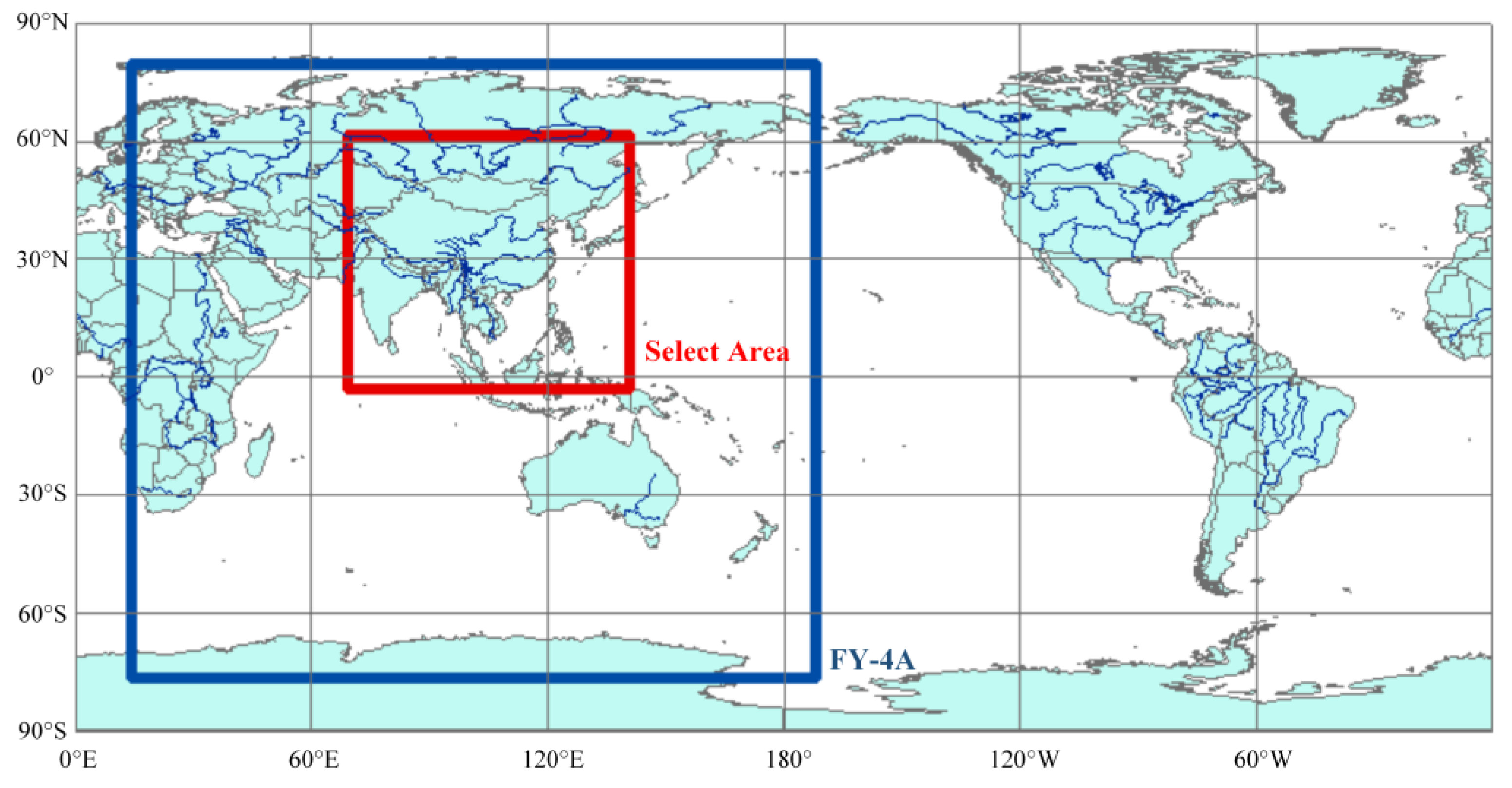
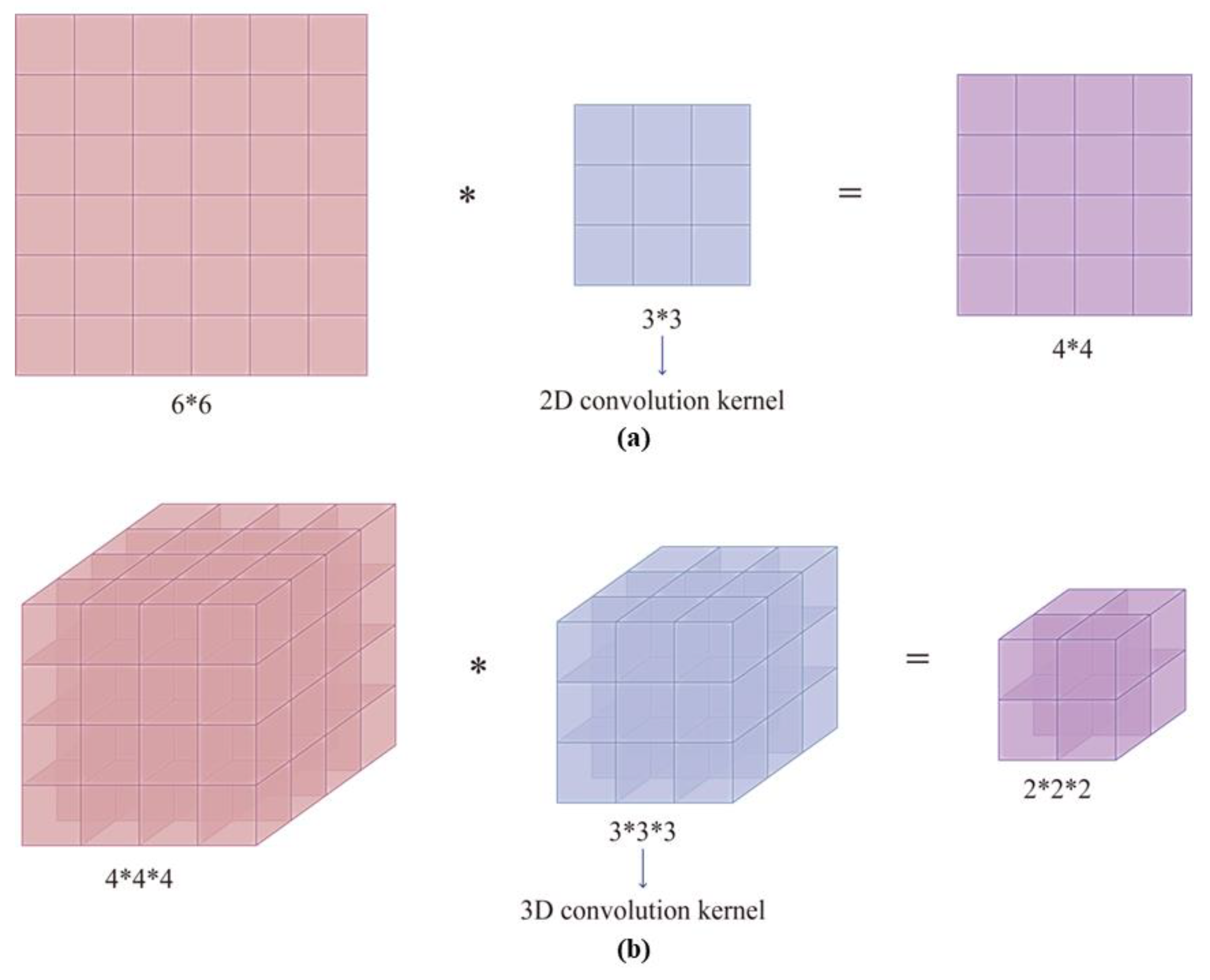
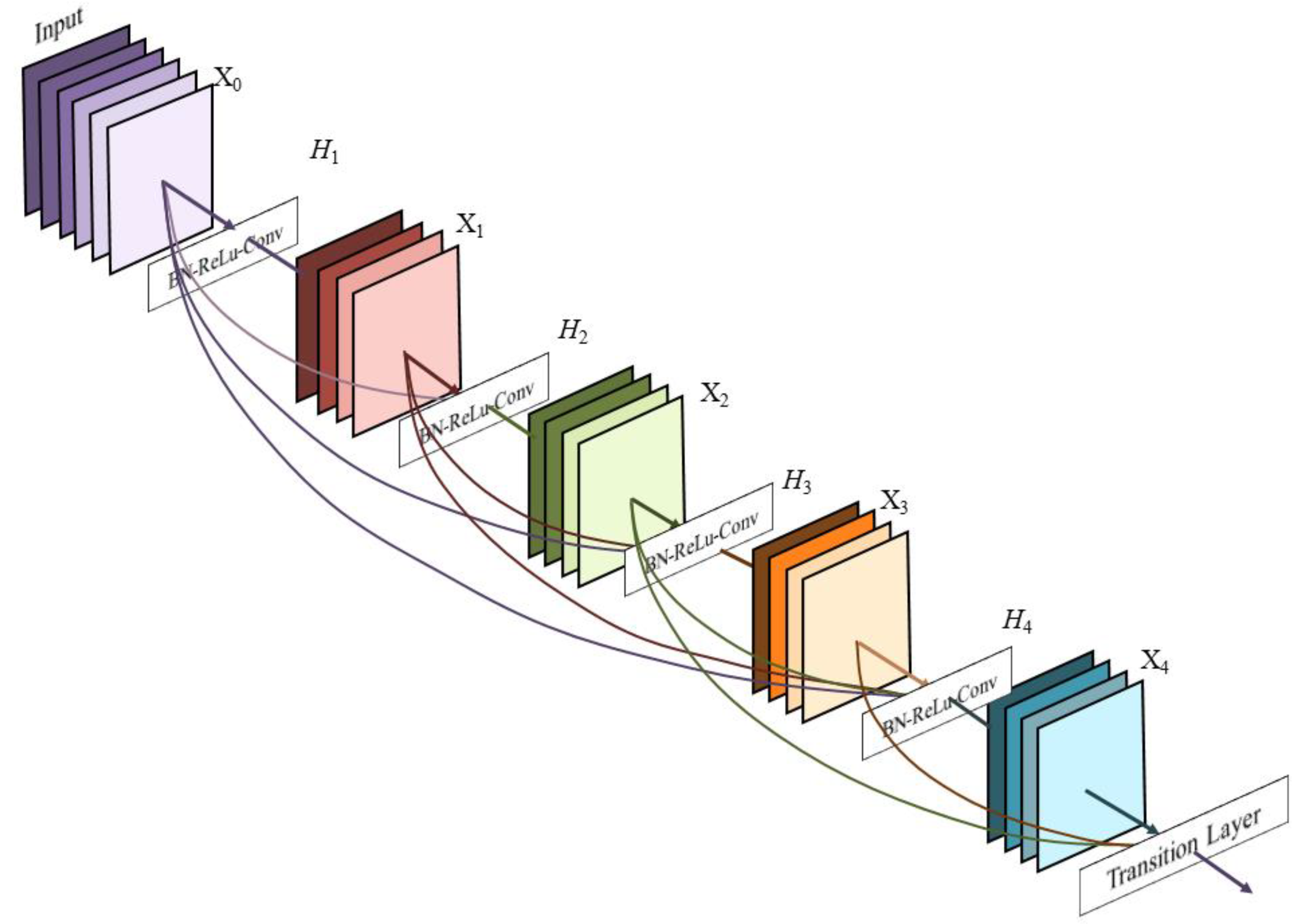
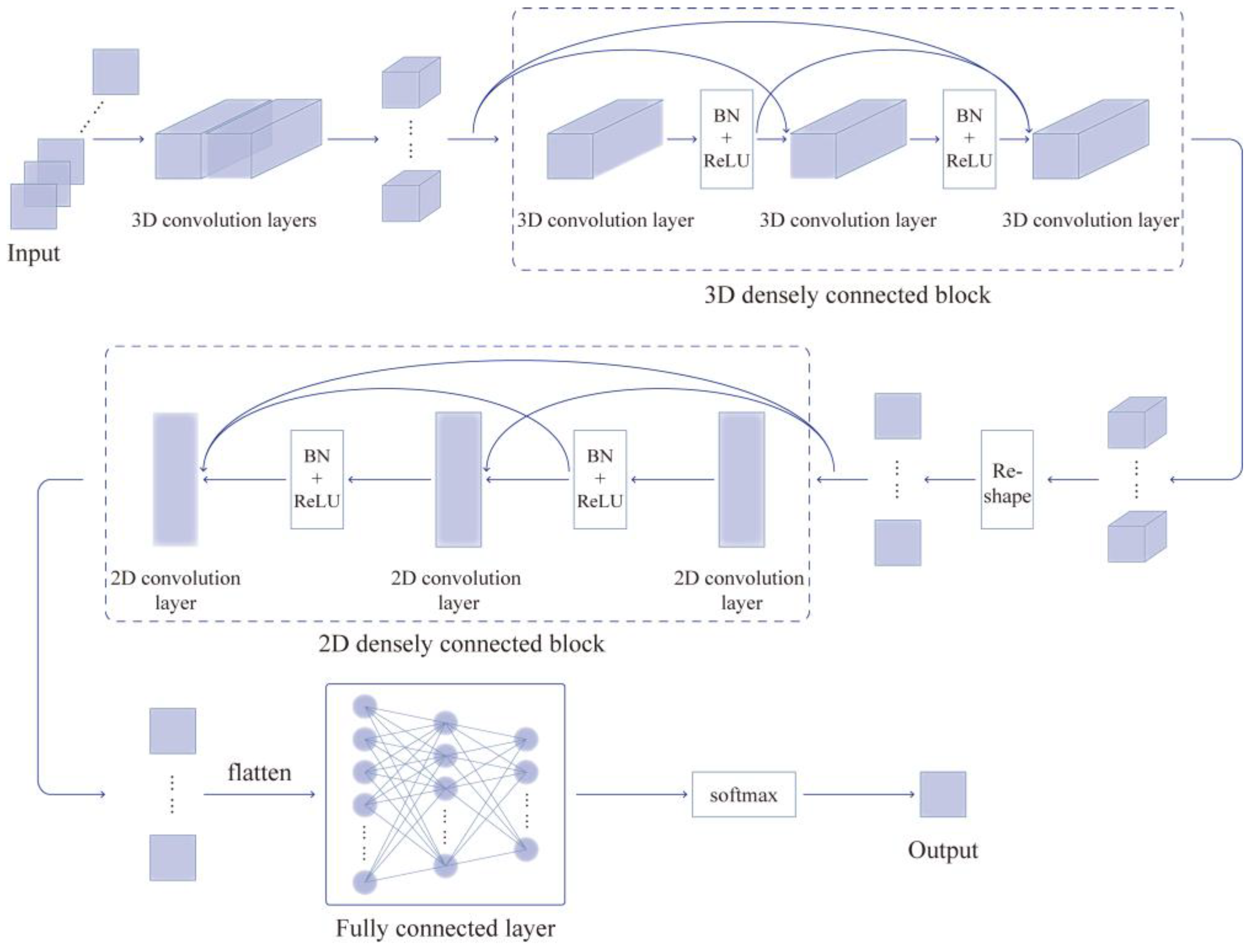
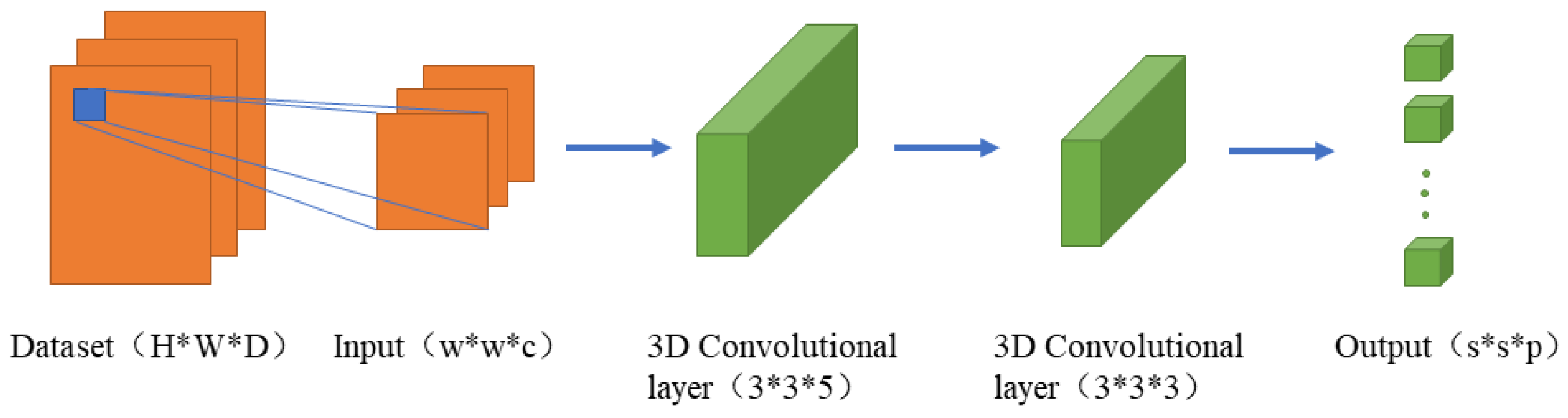
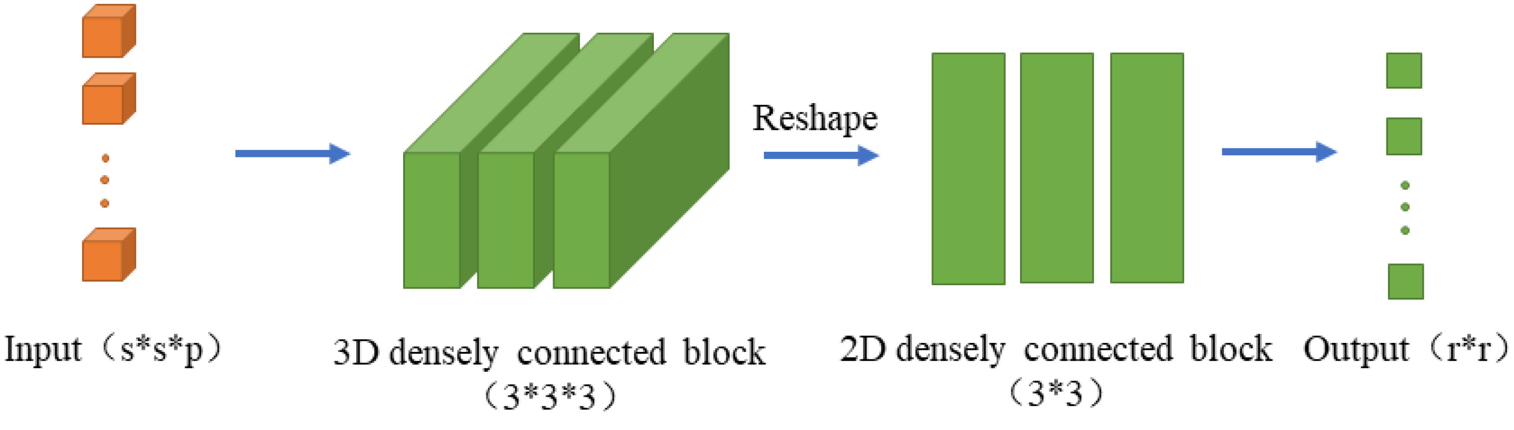
To solve the aforementioned problems, a densely connected hybrid convolutional network (DCHCN) for cloud classification is proposed in this paper. Considering the characteristics of the FY-4A satellite data, three-dimensional (3D) and two-dimensional (2D) convolutional layers are used to mine the spatial–spectral features of the data. Combining the advantages of both convolutions, a hybrid convolution structure was constructed to better extract spatial and spectral features. Additionally, dense connections are constructed to create shortcuts between the front and back layers, which facilitates the back-propagation of the gradient during the training process. By connecting the features of channels, the dense connection technique enables the reuse of features and further improves the classification accuracy. The long time series of FY-4A observations are modeled, and the FY-4A L1-level data are classified pixel-by-pixel into eight categories using the ISCCP cloud classification scheme. The cloud classification products obtained from CloudSat are utilized to evaluate the classification outcome.
The remaining sections of this article are organized as follows. The FY-4A data, CloudSat data for inspection, and data preprocessing are introduced in Section 2. The CNN network, dense connection, and proposed DCHCN methods are discussed in Section 3. The classification results of the datasets and the analysis are presented in Section 4. The article is concluded in Section 5.

2. Data

2.1. FY-4A Data

The advanced geostationary radiation imager (AGRI) carried by the FY-4A outperforms the visible infrared spin scanning radiometer (VISSR) carried by the Fengyun-2 (FY-2) family of spacecraft in terms of coverage, observation accuracy, observation time, and the number of accessible channels. The AGRI has 14 channels ranging from visible to infrared and covering the region from 80.6°N to 80.6°S and from 24.1°E to 174.7°W [33]. The AGRI performs a full scan mode interval of roughly 15 min. It is capable of observing the spectral data of 14 channels, which have various atmospheric features depending on their parameters. Table 1 contains the channel type, central wavelength, and spectral bandwidth for each channel. An example of cloud data from the 14 channels of the FY-4A satellite AGRI detector is presented in Figure 1.

2.2. Cloudsat Data for Inspection

To collect cloud observations, CloudSat was equipped with a cloud profiling radar (CPR), which is a 94-GHz (3.2-mm) sky-bottom radar with a high spatial resolution [34,35,36]. The CloudSat Data Processing Centre (DPC) offers a range of CloudSat products, such as 2B-GEOPROF and 2B-CLDCLASS, which ensure the quality of data evaluation checks and have been utilized in numerous studies over the years [37].
The 2B-CLDCLASS data provide information about the cloud type at each altitude, with the cloud scenario variable in the 2B-CLDCLASS data obtained from the CloudSat satellite allowing for evaluation of the classification results. Each CPR point in these data contains 125 vertical bins; each with a cloud scenario value that identifies the cloud type. Due to the geostationary nature of the FY-4A satellite, it has been challenging to obtain information about the vertical structure of clouds, and previously obtained data only refer to the tops of clouds, making the top cloud types the primary focus. Therefore, the cloud-type data in 2B-CLDCLASS must be preprocessed to obtain single-layer cloud information before being used for top cloud evaluation. Cloud types can be identified only when there are multiple layers with more than two successive levels of the same cloud type. The Dc and Ns cloud types are usually difficult to locate in the topmost layers. When the Dc and Ns cloud types appear in a multilayer cloud, the cloud type is identified as Dc or Ns to distinguish it from other types more clearly and render presentation of the single-layer cloud results easier.

2.3. Data Preprocessing

The 2018–2019 FY-4A AGRI full-disc 4000-m resolution L1 data were preprocessed using data processing techniques, such as cropping, projection conversion, calibration, and spatiotemporal matching, and were used as training data. The data preprocessing process is illustrated in Figure 2. First, the study region was cut, and the column and row numbers of the data were translated to the latitude and longitude values. The selected range was the portion of the territory of China between 0° and 60°N and 70°E and 140°E. The study area is illustrated in Figure 3. The FY-4A full-disk observations were transformed into the corresponding latitude and longitude projections to match the cloud-type data, and the transformed data were interpolated to grid points with a spatial resolution of 0.04° × 0.04°. Then, the visible channel was calibrated to reflectance and the infrared channel to bright temperature according to the calibration factors provided by the FY-4A.
Data obtained from the CloudSat’s 2B–CLDCLASS product during the period 2018–2019 were selected to produce cloud type labels for the FY-4A satellite input data. Since the CloudSat is a polar-orbiting satellite, when the CloudSat data are used for result verification, it is necessary to match the CloudSat data spatially and chronologically with the FY-4A satellite data. When the CPR point and the AGRI point were within 0.04° of each other and when the AGRI point scan time and the CPR scan time were within 15 min from each other, the points were considered prospective matches of the CPR points. The prospective match points were narrowed down to one, and the closest point to the CPR point was selected as a match. This match point was disregarded, and a new matching procedure was initiated if the selected AGRI point data were invalid. Finally, 15,780-pixel samples were obtained, and the precise number of samples for each of the eight categories of clouds (i.e., clear sky, cirrus, altostratus, altocumulus, stratocumulus, cumulus, nimbostratus, and deep-convection) is presented in Table 2.

3. Methods

In this section, the classic techniques, including the 2D-CNN, 3D-CNN, and dense connection, are presented first, and then the proposed DCHCN method is described in detail.

3.1. Superiority of Proposed Module

A CNN is a popular network used for image classification tasks. By performing convolution and pooling, CNN can automatically recognize the spatial features of an image, extracting feature data from various depths by stacking layers [38]. The standard CNN network is a 2D-CNN, and this network was initially created to recognize 2D images. The 2D-CNN structure is shown in Figure 4.
In the 2D-CNN structure, an input image is first convolved using a convolution kernel in the convolution layer. The output of the convolutional layer is then fed to the next layer after being processed using a non-linear function. This process can be expressed as follows:
F l = f ( F l 1 × W l + b l ) ,
where f ( · ) denotes the non-linear activation function, which enhances the network’s ability to handle non-linear data; F l 1 is the input feature map of layer ( l 1 ), and F l is the output feature map of layer l ; W l denotes the convolution filter, and b l is the deviation of the output feature map.
The input feature map is downscaled in the pooling layer to minimize the amount of necessary space. A fully connected layer and a SoftMax classifier have typically been used to determine the final result after several stacked convolution and pooling layers.
The 3D high-level properties of visual data cannot be extracted using the 2D-CNN even though this network can handle 2D graphics well. The 2D-CNN alone is not able to extract good discriminating feature maps from the spectral dimensions. The main reason is the fact that multispectral satellite data are volumetric data and have a spectral dimension as well.
A 3D-CNN model shares many characteristics with a 2D-CNN model but uses 3D convolutional kernels to extract spatial and spectral channel properties from the 3D input data. Similarly, a deep 3D-CNN is more computationally complex. A comparison of the 3D-CNN and 2D-CNN structures is presented in Figure 5.
The above analysis indicates that using only 2D-CNN or 3D-CNN had some limitations, such as the lack of channel relationship information and a complex model. These proposed shortcomings were partially overcome by combining 2D-CNN and 3D-CNN in a hybrid convolutional model. Using the hybrid model, both spectral and spatial feature maps can be fully exploited to achieve optimal classification performance. Table 3 shows the OA and runtime of the 2D-CNN, 3D-CNN, and hybrid convolutional model with the same network parameters, evaluating the benefits and drawbacks of each model.
However, simply stacking convolutional layers does not bring out the best in the network, nor does it make the network deep enough to obtain a better feature map. Huang [39] presented a dense connectivity method and a densely linked convolutional network (DenseNet) model. The main characteristic of dense connections is reusing features by linking them to a channel. As a result, the performance of the model is improved, while requiring fewer computational resources and settings. In the DenseNet, every layer has a direct connection to every layer below it. As a result, the feature maps from all preceding layers are transferred to the lth layer. The specific process can be expressed as follows:
x l = H l ( [ x 0 , x 1 , , x l 1 ] ) ,
where [ x 0 , x 1 , , x l 1 ] refers to the concatenation of the feature maps generated in the zeroth layer and x l is the output.
The dense connection mechanism of the DenseNet model is illustrated in Figure 6.

3.2. Proposed DCHCN Method

The flowchart of the proposed DCHCN method is shown in Figure 7, where it can be seen that the proposed method includes three main components: a 3D-CNN, which is used to extract spatial–spectral information; a hybrid convolutional layer, which includes a 2D-CNN and a 3D-CNN with dense connections; and a fully connected layer, which is used for classification. A detailed explanation of the proposed method is presented in the following.

3.2.1. Using the 3D-CNN for Extracting Spatial–Spectral Features

Convoluting a 3D kernel with 3D data results in a 3D convolution. Two 3D convolution layers are used in the proposed method to extract spatial–spectral information. The activation value of the spatial position (x, y, z) in the jth feature map of the ith layer in the 3D convolution is given by
q i j x y z = f ( m h = 1 H w = 1 W r = 1 R k i j m h w r q ( i 1 ) m ( x + h ) ( y + w ) ( z + r ) + b i j ) ,
where q i j x y z denotes the pixel value at position ( x , y , z ) in the jth feature map of layer i; the 3D convolution kernel size is H × W × R ; m denotes the index of the feature map in layer (i − 1); k i j m h w r denotes the weight of the mth feature map in layer (i − 1) of the 3D convolution kernel; q ( i 1 ) m ( x + h ) ( y + w ) ( z + r ) denotes the pixel value at position ( x + h , y + w , z + r ) in the mth feature map of layer (i − 1); b i j is the bias term; and f ( ) is the activation function.
As shown in Figure 8, it is assumed that the original dataset can be represented as I H × W × C , where H and W denote the length and width of the images in the dataset, respectively, and C is the number of channels of the data in the spectral channel; the number of spectral channels of the data used in this study is 14. In the proposed method, two 3D convolutional layers are used to obtain the joint features containing the spectral information. The spatial–spectral feature extraction steps are as follows:
(1)
To satisfy the 3D-CNN input data format, the original dataset needs to be chunked. Each pixel in the original dataset is traversed, and each pixel is centered to obtain an image block with a size of w × w × c , where w is the width of the image block, i.e., the window size, and c is the number of channels. The label of the input block is equivalent to the label of the center pixel, and the resulting input block is represented by X R w × w × c ;
(2)
For an input block with a size of { w × w × c }, the output with a size of { ( w 2 ) × ( w 2 ) × ( c 4 ) } is obtained by processing the data using eight 3D convolution kernels with a size of { 3 × 3 × 5 }. The first layer of 3D convolution is used to filter the joint spatial spectral features and remove the channels that may contain noise. The second 3D convolution layer consists of 16 convolution kernels with a size of { 3 × 3 × 3 }, extracts the features further, and has an output with a size of { ( w 4 ) × ( w 4 ) × ( c 6 ) }. After two 3D convolutions, the extraction process of 3D features is initially completed. The step size of the above-mentioned convolution layers is one;
(3)
To prevent the network from overfitting and to improve the convergence speed, a batch normalization (BN) layer and a ReLU function are added after each convolution to enhance model robustness.

3.2.2. Hybrid Convolutional Layers with Dense Connections

The 2D-CNN alone is not able to extract good discriminating feature maps from the spectral dimensions. Solving the cloud classification problem using wind cloud data requires extracting both the spectral information hidden in multiple bands and the spatial information.
However, for the satellite cloud classification problem, it is desired to capture both the spectral information encoded in multiple bands and the spatial information. The 3D-CNN kernel can extract spectral–spatial features from data simultaneously, but this significantly increases the computational complexity.
To overcome the disadvantages of using only 2D-CNN or 3D-CNN, this study proposes to combine both networks, leveraging their spectral and spatial feature maps and automatic image-data-feature-learning power to improve accuracy. As illustrated in Figure 9, dense connections are implemented in both 2D-CNN and 3D-CNN to facilitate feature reuse and enhance performance. The steps involved in cloud classification using the hybrid convolutional layers with dense connections are described below:
(1)
The 3D densely connected block includes three convolutional layers, each of which is convolved in 3D. Each layer has a convolutional kernel with a size of { 3 × 3 × 3 } and uses a BN layer and a ReLU function for non-linear transformation between layers to avoid overfitting problems. For the { s × s × p } input, the size of the convolutional layers’ output is guaranteed to be the same by setting the padding to 1 to ensure that the output of each layer can be passed to all subsequent layers. The input is first processed by 16 convolutional kernels with a size of { 3 × 3 × 3 }, and the output is fed to the next layer by splicing it with the input using the concatenate operation (the channel splicing method). To reduce the number of parameters of the 3D densely connected block, the number of output channels is set to 16 for each layer;
(2)
The output obtained using the 3D densely connected block is obtained by screening and capturing the spectral feature information, and the spatial feature map is obtained using 2D convolution. The dimensionality is reduced using the reshape operation to facilitate 2D convolution. The input of size { s × s } is passed through 32 convolution kernels with a size of { 3 × 3 } to extract the spatial features, and the output with a size of { ( s 2 ) × ( s 2 ) } is obtained to construct the input size that can be fed to the 2D densely connected block;
(3)
The 2D densely connected block has three 2D convolutional layers, each of which has a convolutional kernel with a size of { 3 × 3 }, using the BN layer and ReLU function for non-linear transformation between layers to avoid the overfitting problem. For the { ( s 2 ) × ( s 2 ) } input, the output size of the convolutional layers is guaranteed to be the same by setting the padding to one and thus ensuring that the output of each layer can be passed to all subsequent layers. First, the input is passed through 32 convolutional kernels with a size of { 3 × 3 }, and the obtained output is input to the next layer by splicing it with the input performing the concatenation operation (the channel splicing method). For a better exploration of spatial features, the number of output channels is set to 32 for each layer.

3.2.3. Fully Connected Layers for Classification

A SoftMax classifier is employed to classify clouds after flattening the output 2D feature map to a one-dimensional structure and processing it through three fully connected layers. The output layer has the same number of nodes as the number of cloud categories. Table 4 summarizes the layer type, output mapping dimensionality, and parameter count of the proposed model.
In this way, each pixel point corresponds to a probability vector that represents the category that the current pixel belongs to. The category of the pixel point is determined by the probability of the current pixel performing the pixel-by-pixel cloud classification.

3.3. Model Training

The 2018–2019 FY-4A AGRI full-disk 4000-m resolution L1 data were labeled utilizing 2018–2019 CloudSat’s 2B-CLDCLASS product data. The data were divided into training and test sets in a 7:3 ratio with the elimination of unreliable and missing data through the preprocessing methods outlined in Section 2.2 and Section 2.3. The dataset was created using data with intervals greater than half an hour to avoid minor cloud shifts and reduce model accuracy caused by short intervals. The time range of the dataset ranged from 00:00 UTC to 09:00 UTC with 11,046 samples in the training dataset and 4734 samples in the test dataset. The cube-shaped input data for FY-4A were created using small, overlapping cubic blocks with labels assigned to the central pixels. A total of 120 training epochs were conducted using the Adam optimizer. The model was trained in batches of 14 × 43 × 43.
Figure 10 illustrates the production of the input image blocks in the training set. A total of 14 channels of images from FY-4A (simplified as RGB images in the figure) were spatiotemporally matched with CloudSat satellite data to obtain matching points and assigned labels. Using the matched points as the central pixel, their neighbors were taken to form the input image block of the training set, and the labels of the image block were consistent with those of the central pixel.

4. Result and Analysis

This section analyzes the effects of two main parameters, namely the spatial size of the input block, and the number of spectral channel dimensions of the output feature map of the 3D-CNN, of the proposed DCHCN on its classification performance. The experimental results of the proposed method and several state-of-the-art methods are presented and analyzed. The three metrics OA (overall accuracy), AA (average accuracy) and Kappa (kappa coefficient) are used in this paper to analyze and evaluate the performance of the model. OA indicates the ratio of the number of samples correctly predicted by the model to the total number of samples, AA denotes the average of the model’s prediction accuracy for each category, and Kappa indicates the agreement between the model prediction results and the actual classification results, taking into account the random classification.

4.1. Experimental Configuration

The Windows 10 operating system was used in all tests. The tests were conducted on computers with a 12th Gen Intel(R) Core (TM) i5-12400F CPU and an Nvidia GeForce RTX3060 Ti GPU using PyTorch 1.2.0 deep learning framework and Python 3.9. The number and distribution of training and test dataset samples are presented in Table 5.

4.2. Analysis of Parameter Effects on Model Performance

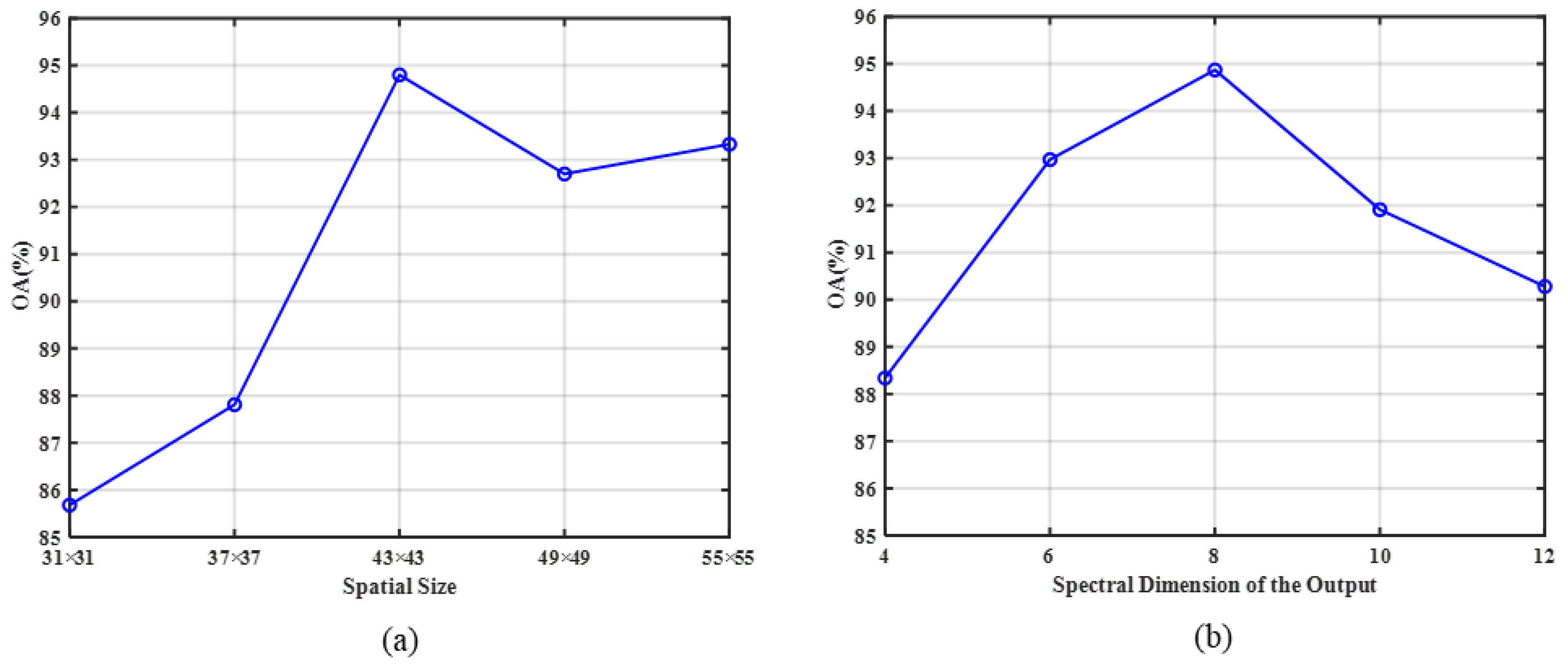
4.2.1. Spatial Size Effect

The spatial size of the input block defines the amount of spatial feature information in the input block, and, in CNNs, the effective feature information can significantly affect the classification performance. Therefore, in this study, the spatial size of the input block was analyzed experimentally. In this experiment, the spatial size of the input block was set to {31 × 31, 37 × 37, 43 × 43, 49 × 49, 55 × 55}. The experimental results are presented in Figure 11a.
As shown in Figure 11a, the OA value gradually increased when the spatial size increased from 31 to 43, but as the spatial size continued to increase, OA showed a decreasing trend. The increase in spatial size could improve the spatial feature information obtained by the network to a certain extent, but a too-large spatial size could reduce the classification performance of the network. Additionally, a too-large size could lead to the introduction of other types of pixels and even cause noise. Therefore, to achieve the best classification results, a size of {43 × 43} was selected for the input block of the network.

4.2.2. Spectral Dimension of the 3D-CNN Output Feature Map

The input data were processed using the 3D-CNN to extract the spectral–spatial features first, before the data entered the hybrid convolution layer. The output feature map of the 3D-CNN could affect the final feature information obtained using hybrid convolution and thus affect the classification results. Therefore, the effect of the spectral channel dimension of the 3D-CNN output feature map was examined experimentally by changing the 3D-CNN convolution kernel size. In this experiment, the output feature map’s spectral channel dimensions of the 3D-CNN were set to {4,6,8,10,12}. The experimental results are presented in Figure 11b.

4.3. Results, Analysis, and Comparison of Different Cloud Classification Models

A variety of deep learning networks were selected for the comparison experiments. The proposed DCHCN model was compared with the 2D-CNN, 3D-CNN, HybridSN, UNet, and U2Net models. All models in the comparison experiments were trained and tested on the same training and test datasets. In addition, for all models the training included 120 epochs, and the same parameters, including the optimizer type, loss function, and learning rate, were used in the training process to obtain the final classification models. The eight cloud types are labeled in the following order: Clear sky, Ci, As, Ac, Sc, Cu, Ns, and Dc. The performance of the six models in the cloud classification task was tested separately, and their performances are presented in Table 5.
As shown in Table 6, The numbers in bold indicate the models that achieved the best results in their category, the proposed DCHCN model obtained the highest OA, AA, and Kappa values among all models. Although the 2D-CNN, 3D-CNN, HybridSN, UNet, and U2Net models were designed with different network structures to obtain high classification performance, the proposed model benefited from the combination of 2D and 3D convolutions, which resulted in a better classification performance. The proposed method combined spatial and spectral feature information and used dense connections to reuse the features better, and thus could achieve better results at a lower computational cost.
Specifically, the 2D-CNN had the worst classification results among all models for all classes, except for clear sky; i.e., its classification accuracy was below 60% for some of the classes. This model also had the smallest OA, AA, and Kappa values due to the unavailability of spectral feature information for classification. The 3D-CNN model had better classification results compared to the 2D-CNN model, but required more time to obtain these results. The HybridSN model used a hybrid convolutional architecture similar to that of the proposed method. The hybrid convolutional architecture provided high accuracy of 3D convolution while minimizing the number of model parameters. The UNet and U2Net used deeper 2D convolution and could extract feature information better by using the U-shaped structure. However, purely 2D convolution with an increased depth was still not enough to compete with the proposed method.
Moreover, in most cases, the proposed method performed better than the other methods regarding the classification accuracy for all types of clouds. Specifically, the cloud types Ac, Sc, and Dc that had more structural changes could be easily confused with other cloud types, so it was more difficult to classify them accurately. Still, the proposed method performed better than the other methods on these classes. This was mainly due to the fact that the proposed model used dense connections to connect the layers, while the HybridSN model used hybrid convolution. By building a dense connection module, the hidden spectral information, as well as spatial information, could be explored better, and the useful feature information obtained from the other layers could be retained, thus achieving accurate classification of cloud types with insignificant feature information. In addition, compared to the UNet and U2Net models, the proposed method did not use relatively deep convolutional layers and thus did not introduce additional time overhead while improving the classification accuracy; the proposed method had obvious advantages in time performance compared to the other models.
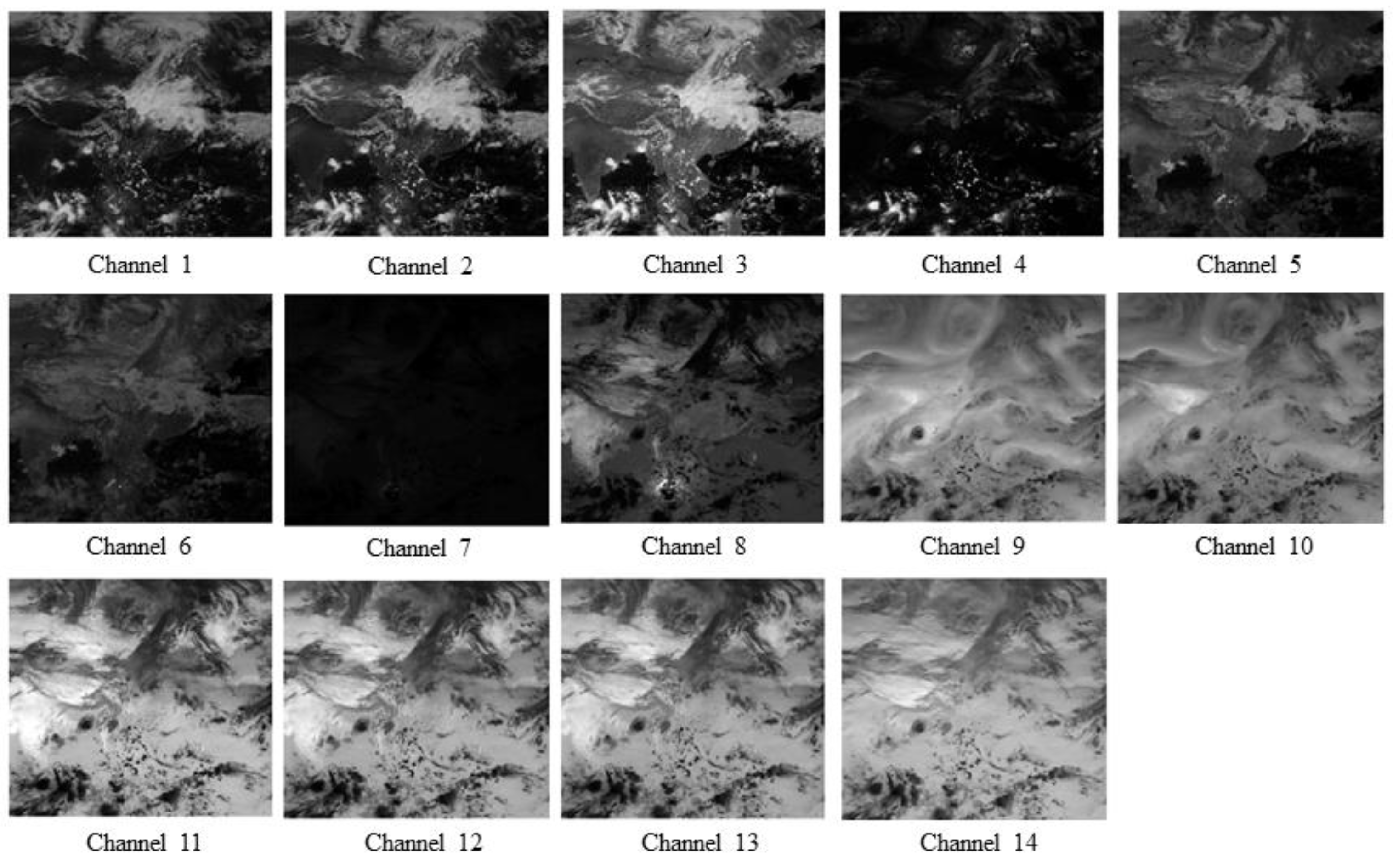
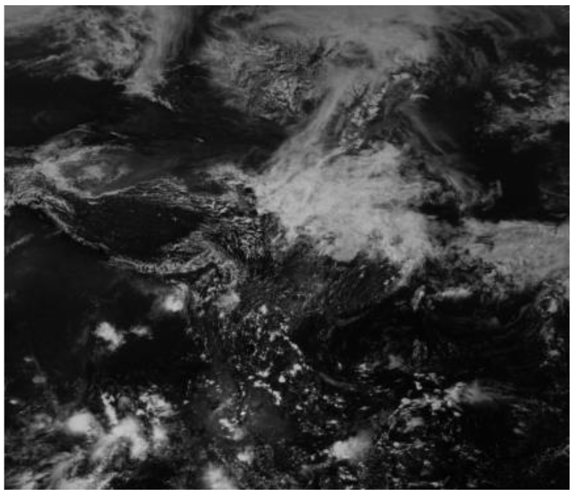
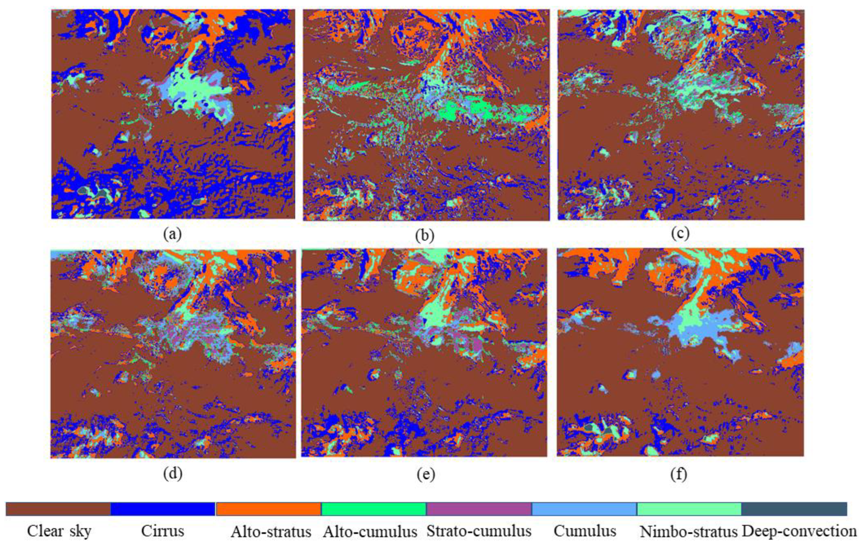
Figure 12 shows the original satellite cloud image, and Figure 13 depicts the corresponding classification results of each classification method on a dataset. The satellite cloud map data collection time used for the presentation of classification results was 5:45 a.m. on 21 May 2018. At this time, all types of clouds are represented in satellite cloud images.
The classification-result analysis showed that the classification maps obtained using the 2D-CNN and 3D-CNN included more misclassifications than the other models. The HybridSN, UNet, and U2Net classification maps provided clouds that were more fragmented, and they could not distinguish cloud categories Ac, As, Cu, and Ci well. This is because these maps could not use spectral information more accurately than the proposed model. Finally, the classification map obtained using the proposed method could ensure the integrity of cloud clusters, relatively smooth boundaries, high performance, and accurate classification results.
The cloud map data used for the proposed classification model verification corresponded to the spring season, when the probability of single-layer clouds in mainland China is high, especially in the southern region. According to previous macroscopic studies on cloud types in China, the probability of high clouds in the tropic regions is the highest, which is indicated by a large portion of high clouds, such as Ci and As, at the bottom of the classification map. However, in mainland China, the probability of high clouds in the north, especially the northeast and north of China, is higher than that in the south, which is indicated by a large number of high clouds, such as Ci and As, at the top of the classification map. In addition, in the tropical region, deep convective activity is more frequent, and water vapor is more abundant, which results in a higher probability of producing highly unstable deep convective clouds of the Dc type and extendable rain clouds of the Ns type. The probability of medium clouds in the southwest region is higher than 50%, which is mainly demonstrated in the classification chart as Sc and Ac cloud types in this region. However, in the sea in the south, at 20°N, the probability of medium clouds is very low and is thus almost not reflected in the classification chart. Due to the influence of water vapor, large cumulus (Cu) clouds also appear in the classification map. Thus, the classification map obtained using the proposed method is consistent with the findings of macroscopic studies in the Chinese region.

5. Conclusions

This paper proposes a densely connected hybrid convolutional network (DCHCN) for cloud classification tasks using FY-4 satellite data. The proposed DCHCN approach combines 3D and 2D convolutions to integrate spectral and spatial feature information, which effectively improves cloud classification accuracy. Moreover, the proposed approach employs dense connections and fully connected layers to further enhance classification performance. Experimental results demonstrate that the proposed method outperforms other comparative models and attains the highest classification accuracy. These findings confirm the efficiency and advantages of the proposed method in cloud classification using FY-4 satellite data.
However, there are still some aspects that require further improvement. Although the proposed method combines convolutional layers to exploit spatial and spectral features more effectively, it is observed that network performance varies significantly with different spatial scales or spectral dimensions of the parameters in parameter analysis experiments. Furthermore, the optimal parameters found in the experiments may not be applicable to other datasets, indicating the need for further research on the spatial and spectral properties of clouds to improve network robustness. In terms of dataset, the training process is limited by CloudSat’s running orbit and running time, which makes it challenging to incorporate more accurate cloud classification data. Additionally, the inherent nature of satellite data may cause CloudSat’s data to deviate from the real situation. As CloudSat does not provide data labels over a continuous time, the study did not consider the temporal dimension. In addition, the top height of the cloud type St is low, the distribution is scattered and fragmented, and there is a severe problem of insufficient samples. This cloud type was not included in this study. Therefore, in future studies, the dataset will be enhanced by including measured data over a continuous time to improve the accuracy and aid in the analysis. Additionally, a classification scheme for the St type will be added to further improve cloud classification accuracy. Further improvements in the classification accuracy of specific cloud types could eventually lead to overall improvements in the cloud type classification of the proposed model.

Author Contributions

Conceptualization: B.W. and M.Z.; methodology: B.W., M.Z., W.C. and Y.C.; software: B.W. and M.Z.; validation: B.W., M.Z. and Q.S.; formal analysis: B.W., M.Z. and W.C.; original manuscript writing and preparation: M.Z.; manuscript—review and editing: B.W., M.Z., J.L. and L.W.; visualization: M.Z. and Y.C.; supervision: Q.S., W.C. and J.L. All authors have read and agreed to the published version of the manuscript.

Funding

This research was funded by the Space Optoelectronic Measurement and Perception Laboratory of BICE (grant no. LabSOMP-2021-06) and the Natural Science Foundation of Jiangsu Province (No. BK20220888).

Data Availability Statement

Not applicable.

Acknowledgments

The authors would like to thank the China National Satellite Meteorological Center and the CloudSat data website, which are freely accessible to the public.

Conflicts of Interest

The authors declare no conflict of interest.

References

  1. Hunt, G.E. On the sensitivity of a general circulation model climatology to changes in cloud structure and radiative properties. Tellus A Dyn. Meteorol. Oceanogr. 1982, 34, 29. [Google Scholar] [CrossRef]
  2. Baker, M. Cloud microphysics and climate. Science 1997, 276, 1072–1078. [Google Scholar] [CrossRef]
  3. Liu, Y.; Xia, J.; Shi, C.X.; Hong, Y. An Improved Cloud Classification Algorithm for China’s FY-2C Multi-Channel Images Using Artificial Neural Network. Sensors 2009, 9, 5558–5579. [Google Scholar] [CrossRef]
  4. Gan, J.; Lu, W.; Li, Q.; Zhang, Z.; Yang, J.; Ma, Y.; Yao, W. Cloud Type Classification of Total-Sky Images Using Duplex Norm-Bounded Sparse Coding. IEEE J. Sel. Top. Appl. Earth Obs. Remote Sens. 2017, 10, 3360–3372. [Google Scholar] [CrossRef]
  5. Stubenrauch, C.J.; Rossow, W.B.; Kinne, S.; Ackerman, S.; Cesana, G.; Chepfer, H.; Di Girolamo, L.; Getzewich, B.; Guignard, A.; Heidinger, A.; et al. Assessment of Global Cloud Datasets from Satellites: Project and Database Initiated by the GEWEX Radiation Panel. Bull. Am. Meteorol. Soc. 2013, 94, 1031–1049. [Google Scholar] [CrossRef]
  6. Reichstein, M.; Camps-Valls, G.; Stevens, B.; Jung, M.; Denzler, J.; Carvalhais, N.; Prabhat. Deep learning and process understanding for data-driven Earth system science. Nature 2019, 566, 195–204. [Google Scholar] [CrossRef] [PubMed]
  7. Huertas-Tato, J.; Rodríguez-Benítez, F.J.; Arbizu-Barrena, C.; Aler-Mur, R.; Galvan-Leon, I.; Pozo-Vázquez, D. Automatic Cloud-Type Classification Based On the Combined Use of a Sky Camera and a Ceilometer. J. Geophys. Res. Atmos. 2017, 122, 11045–11061. [Google Scholar] [CrossRef]
  8. Li, J.; Menzel, W.P.; Yang, Z.; Frey, R.A.; Ackerman, S.A. High-spatial-resolution surface and cloud-type classification from MODIS multispectral band measurements. J. Appl. Meteorol. Climatol. 2003, 42, 204–226. [Google Scholar] [CrossRef]
  9. Wang, J.; Liu, C.; Yao, B.; Min, M.; Letu, H.; Yin, Y.; Yung, Y.L. A multilayer cloud detection algorithm for the Suomi-NPP Visible Infrared Imager Radiometer Suite (VIIRS). Remote Sens. Environ. 2019, 227, 1–11. [Google Scholar] [CrossRef]
  10. Rossow, W.B.; Schiffer, R.A. ISCCP cloud data products. Bull. Am. Meteorol. Soc. 1991, 72, 2–20. [Google Scholar] [CrossRef]
  11. Hahn, C.J.; Rossow, W.B.; Warren, S.G. ISCCP cloud properties associated with standard cloud types identified in individual surface observations. J. Clim. 2001, 14, 11–28. [Google Scholar] [CrossRef]
  12. Austin, R.T.; Heymsfield, A.J.; Stephens, G.L. Retrieval of ice cloud microphysical parameters using the CloudSat millimeter-wave radar and temperature. J. Geophys. Res. 2009, 114. [Google Scholar] [CrossRef]
  13. Powell, K.A.; Hu, Y.; Omar, A.; Vaughan, M.A.; Winker, D.M.; Liu, Z.; Hunt, W.H.; Young, S.A. Overview of the CALIPSO Mission and CALIOP Data Processing Algorithms. J. Atmos. Ocean. Technol. 2009, 26, 2310–2323. [Google Scholar] [CrossRef]
  14. Kahn, B.; Chahine, M.; Stephens, G.; Mace, G.; Marchand, R.; Wang, Z.; Barnet, C.; Eldering, A.; Holz, R.; Kuehn, R. Cloud type comparisons of AIRS, CloudSat, and CALIPSO cloud height and amount. Atmos. Chem. Phys. 2008, 8, 1231–1248. [Google Scholar] [CrossRef]
  15. Yan, W.; Han, D.; Zhou, X.K.; Liu, H.F.; Tang, C. Analysing the structure characteristics of tropical cyclones based on CloudSat satellite data. Chin. J. Geophys. 2013, 56, 1809–1824. [Google Scholar] [CrossRef]
  16. Subrahmanyam, K.V.; Kumar, K.K.; Tourville, N.D. CloudSat Observations of Three-Dimensional Distribution of Cloud Types in Tropical Cyclones. IEEE J. Sel. Top. Appl. Earth Obs. Remote Sens. 2018, 11, 339–344. [Google Scholar] [CrossRef]
  17. Li, G.L.; Yan, W.; Han, D.; Wang, R.; Ye, J. Applications of the CloudSat Tropical Cyclone Product in Analyzing the Vertical Structure of Tropical Cyclones over the Western Pacific. J. Trop. Meteorol. 2017, 23, 473–484. [Google Scholar] [CrossRef]
  18. Bankert, R.L.; Mitrescu, C.; Miller, S.D.; Wade, R.H. Comparison of GOES cloud classification algorithms employing explicit and implicit physics. J. Appl. Meteorol. Climatol. 2009, 48, 1411–1421. [Google Scholar] [CrossRef]
  19. Mouri, K.; Izumi, T.; Suzue, H.; Yoshida, R. Algorithm Theoretical Basis Document of cloud type/phase product. Meteorol. Satell. Cent. Tech. Note 2016, 61, 19–31. [Google Scholar]
  20. Suzue, H.; Imai, T.; Mouri, K. High-resolution cloud analysis information derived from Himawari-8 data. Meteorol. Satell. Cent. Tech. Note 2016, 61, 43–51. [Google Scholar]
  21. Ackerman, S.A.; Strabala, K.I.; Menzel, W.P.; Frey, R.A.; Moeller, C.C.; Gumley, L.E. Discriminating clear sky from clouds with MODIS. J. Geophys. Res. Atmos. 1998, 103, 32141–32157. [Google Scholar] [CrossRef]
  22. Purbantoro, B.; Aminuddin, J.; Manago, N.; Toyoshima, K.; Lagrosas, N.; Sumantyo, J.T.S.; Kuze, H. Comparison of Cloud Type Classification with Split Window Algorithm Based on Different Infrared Band Combinations of Himawari-8 Satellite. Adv. Remote Sens. 2018, 7, 218–234. [Google Scholar] [CrossRef]
  23. Poulsen, C.; Egede, U.; Robbins, D.; Sandeford, B.; Tazi, K.; Zhu, T. Evaluation and comparison of a machine learning cloud identification algorithm for the SLSTR in polar regions. Remote Sens. Environ. 2020, 248, 111999. [Google Scholar] [CrossRef]
  24. Ebert, E.E. Analysis of polar clouds from satellite imagery using pattern recognition and a statistical cloud analysis scheme. J. Appl. Meteorol. Climatol. 1989, 28, 382–399. [Google Scholar] [CrossRef]
  25. Berendes, T.A.; Mecikalski, J.R.; MacKenzie, W.M.; Bedka, K.M.; Nair, U.S. Convective cloud identification and classification in daytime satellite imagery using standard deviation limited adaptive clustering. J. Geophys. Res. 2008, 113. [Google Scholar] [CrossRef]
  26. Zhang, C.; Yu, F.; Wang, C.; Yang, J. Three-dimensional extension of the unit-feature spatial classification method for cloud type. Adv. Atmos. Sci. 2011, 28, 601–611. [Google Scholar] [CrossRef]
  27. Gao, T.; Zhao, S.; Chen, F.; Sun, X.; Liu, L. Cloud Classification Based on Structure Features of Infrared Images. J. Atmos. Ocean. Technol. 2011, 28, 410–417. [Google Scholar] [CrossRef]
  28. Gomez-Chova, L.; Camps-Valls, G.; Bruzzone, L.; Calpe-Maravilla, J. Mean Map Kernel Methods for Semisupervised Cloud Classification. IEEE Trans. Geosci. Remote Sens. 2010, 48, 207–220. [Google Scholar] [CrossRef]
  29. Heinle, A.; Macke, A.; Srivastav, A. Automatic cloud classification of whole sky images. Atmos. Meas. Tech. 2010, 3, 557–567. [Google Scholar] [CrossRef]
  30. Taravat, A.; Del Frate, F.; Cornaro, C.; Vergari, S. Neural Networks and Support Vector Machine Algorithms for Automatic Cloud Classification of Whole-Sky Ground-Based Images. IEEE Geosci. Remote Sens. Lett. 2015, 12, 666–670. [Google Scholar] [CrossRef]
  31. Zhang, J.; Liu, P.; Zhang, F.; Song, Q. CloudNet: Ground-Based Cloud Classification With Deep Convolutional Neural Network. Geophys. Res. Lett. 2018, 45, 8665–8672. [Google Scholar] [CrossRef]
  32. Jiang, Y.; Cheng, W.; Gao, F.; Zhang, S.; Wang, S.; Liu, C.; Liu, J. A Cloud Classification Method Based on a Convolutional Neural Network for FY-4A Satellites. Remote Sens. 2022, 14, 2314. [Google Scholar] [CrossRef]
  33. Guo, Q.; Lu, F.; Wei, C.; Zhang, Z.; Yang, J. Introducing the New Generation of Chinese Geostationary Weather Satellites, Fengyun-4. Bull. Am. Meteorol. Soc. 2017, 98, 1637–1658. [Google Scholar] [CrossRef]
  34. Hawkins, J.; Miller, S.; Mitrescu, C.; L’Ecuyer, T.; Turk, J.; Partain, P.; Stephens, G. Near-Real-Time Applications of CloudSat Data. J. Appl. Meteorol. Climatol. 2008, 47, 1982–1994. [Google Scholar] [CrossRef]
  35. Sassen, K.; Wang, Z.; Liu, D. Global distribution of cirrus clouds from CloudSat/Cloud-Aerosol Lidar and Infrared Pathfinder Satellite Observations (CALIPSO) measurements. J. Geophys. Res. 2008, 113(D8). [Google Scholar] [CrossRef]
  36. Stephens, G.L.; Vane, D.G.; Tanelli, S.; Im, E.; Durden, S.; Rokey, M.; Reinke, D.; Partain, P.; Mace, G.G.; Austin, R.; et al. CloudSat mission: Performance and early science after the first year of operation. J. Geophys. Res. 2008, 113. [Google Scholar] [CrossRef]
  37. Vane, D.; Stephens, G.L. The CloudSat Mission and the A-Train: A Revolutionary Approach to Observing Earth’s Atmosphere. In Proceedings of the 2008 IEEE Aerospace Conference, Big Sky, MT, USA, 1–8 March 2008; pp. 1–5. [Google Scholar]
  38. Gu, J.; Wang, Z.; Kuen, J.; Ma, L.; Shahroudy, A.; Shuai, B.; Liu, T.; Wang, X.; Wang, G.; Cai, J.; et al. Recent advances in convolutional neural networks. Pattern Recognit. 2018, 77, 354–377. [Google Scholar] [CrossRef]
  39. Huang, G.; Liu, Z.; Van Der Maaten, L.; Weinberger, K.Q. Densely connected convolutional networks. In Proceedings of the IEEE Conference on Computer Vision and Pattern Recognition, Honolulu, HI, USA, 21–26 July 2017; pp. 4700–4708. [Google Scholar]
Figure 1. Examples of the advanced geostationary radiation imager’s 14-channel observation images.
Remotesensing 15 02673 g001
Figure 2. Illustration of the data preprocessing process.
Remotesensing 15 02673 g002
Figure 3. Illustration of the selected area and the observation area of the FY-4A satellite.
Remotesensing 15 02673 g003
Figure 4. Basic 2D-CNN structure.
Remotesensing 15 02673 g004
Figure 5. Schematics of the convolution calculation: (a) 2D-CNN; (b) 3D-CNN.
Remotesensing 15 02673 g005
Figure 6. The Dense connection mechanism of DenseNet.
Remotesensing 15 02673 g006
Figure 7. Flowchart of our proposed model.
Remotesensing 15 02673 g007
Figure 8. Using the 3D-CNN for extracting the spatial–spectral features.
Remotesensing 15 02673 g008
Figure 9. Hybrid convolutional layers with a dense connection.
Remotesensing 15 02673 g009
Figure 10. Image data for model training. The two diagrams on the left show the raw FY-4A data and the matching points with the corresponding colored boxes marked with the label positions, selected according to the color scale in the legend. The figure on the right shows a zoomed-in example of the training set data from the left figure.
Remotesensing 15 02673 g010
Figure 11. Classification results obtained under different experimental conditions: (a) Classification results obtained at different spatial sizes; (b) classification results obtained for different spectral dimensions of the output. In (b) it can be seen that, starting from four spectral dimensions, the OA reached the maximum for eight spectral dimensions. With a further increase in the spectral dimension based on eight spectral dimensions, the OA started to decrease. This indicated that with the increase in spectral dimension number, the noise information also increased gradually, which affected the acquisition of spectral feature information and led to a decrease in classification accuracy. According to the experimental results, the number of spectral channel dimensions of the 3D-CNN output feature map was set to eight.
Remotesensing 15 02673 g011
Figure 12. Original FY-4A satellite cloud image data collected at 5:45 a.m. on 21 May 2018.
Remotesensing 15 02673 g012
Figure 13. Classification maps obtained using classification methods on the dataset: (a) 2D-CNN; (b) 3D-CNN; (c) HybridSN; (d) UNet; (e) U2Net; (f) proposed DCHCN.
Remotesensing 15 02673 g013
Table 1. FY-4A satellite parameters.
Channel NumberChannel TypeCentral WavelengthSpectral Bandwidth
1VIS/NIR0.47 µm0.45–0.49 µm
20.65 µm0.55–0.75 µm
30.825 µm0.75–0.90 µm
4Shortwave IR1.375 µm1.36–1.39 µm
51.61 µm1.58–1.64 µm
62.25 µm2.1–2.35 µm
7Midwave IR3.75 µm3.5–4.0 µm (high)
83.75 µm3.5–4.0 µm (low)
9Water vapor6.25 µm5.8–6.7 µm
107.1 µm6.9–7.3 µm
11Longwave IR8.5 µm8.0–9.0 µm
1210.7 µm10.3–11.3 µm
1312.0 µm11.5–12.5 µm
1413.5 µm13.2–13.8 µm
Table 2. Sample distribution of the dataset.
CategoryNameNumber of Samples
1Clear sky6447
2Cirrus2553
3Altostratus3260
4Altocumulus723
5Stratocumulus530
6Cumulus540
7Nimbostratus1550
8Deep-convection177
Table 3. The OA and runtime of the 2D-CNN, 3D-CNN, and hybrid convolutional model with the same network parameters.
2D-CNN3D-CNNThe Hybrid Convolutional Model
OA87.3590.8592.01
Runtime (s)192.6338.7252.8
Table 4. Detailed information on the layer structure and parameters of the proposed model.
LayerTypeOutput ShapeParameter
Input_1/(43, 43, 14, 1)0
Conv3d_13 × 3 × 5 Conv3D(41, 41, 10, 8)368
Conv3d_23 × 3 × 3 Conv3D(39, 39, 8, 16)3472
Dense Block 3d_1[3 × 3 × 3 Conv3D] × 3(39, 39, 8, 16)41,520
Reshape_1Reshape(39, 39, 128)0
Conv2d_13 × 3 Conv2D(37, 37, 32)36,896
Dense Block 2d_1[3 × 3 Conv2D] × 3(37, 37, 32)55,392
Flatten_1Flatten(43,808)0
Dense_1Dense(256)11,215,104
Dropout_1Dropout(256)0
Dense_2Dense(128)32,896
Dropout_2Dropout(128)0
Dense_3Dense(8)1032
Table 5. Data distribution of the training and test datasets.
CategoryNameNumber of Training SamplesNumber of Test SamplesNumber of Samples
1Clear sky451319346447
2Cirrus17877662553
3Altostratus22829783260
4Altocumulus506217723
5Stratocumulus371159530
6Cumulus378162540
7Nimbostratus10854651550
8Deep-convection12453177
Acc.11,046473415,780
Table 6. Classification results of the classification methods.
Category2D-CNN3D-CNNHybridSNUNetU2NetDCHCN
197.2695.5595.0996.4397.3197.10
275.2086.6886.8190.8691.1293.60
389.6789.9894.8989.9892.4395.30
459.9170.0575.5877.4276.9682.95
555.9775.4779.8773.5883.0288.05
675.8392.5993.8395.6892.5998.15
791.4095.4893.3393.9896.1397.85
864.1581.1383.0284.9186.7986.49
OA87.3590.8591.9592.1693.4995.20
AA76.1985.8787.8087.8589.5492.47
Kappa82.7687.7889.2289.5091.3093.60
Disclaimer/Publisher’s Note: The statements, opinions and data contained in all publications are solely those of the individual author(s) and contributor(s) and not of MDPI and/or the editor(s). MDPI and/or the editor(s) disclaim responsibility for any injury to people or property resulting from any ideas, methods, instructions or products referred to in the content.

