Article

Sensitivity of Vegetation to Climate in Mid-to-High Latitudes of Asia and Future Vegetation Projections

1
Collaborative Innovation Center on Forecast and Evaluation of Meteorological Disasters, Nanjing University of Information Science and Technology, Nanjing 210044, China
2
School of Atmospheric Sciences, Nanjing University of Information Science and Technology, Nanjing 210044, China
3
Huangpi District Meteorological Bureau, Wuhan 430300, China
*
Author to whom correspondence should be addressed.
These authors contributed equally to this work and should be considered co-first authors.
Remote Sens. 2023, 15(10), 2648; https://doi.org/10.3390/rs15102648
Submission received: 27 March 2023 / Revised: 11 May 2023 / Accepted: 16 May 2023 / Published: 19 May 2023

Abstract

:
Mid- to high-latitude Asia (MHA) is one of the regions with the strongest warming trend and it is also a region where ecosystems are most sensitive to climate variability. However, how the vegetation in the region will change in the future remains uncertain. Using observation-based Leaf Area Index (LAI) and meteorological data and the multiple regression method, this study analyzes the response of vegetation in the MHA to climate elements during 1982–2020. Then, machine learning prediction models based on the Random Forest (RF) and Extreme Random Tree (ERT) algorithms are built and validated. Based on the calibrated meteorological fields from 17 Coupled Model Intercomparison Project Phase 6 (CMIP6) models under intermediate (SSP2-4.5) and high (SSP5-8.5) emission scenarios and the machine learning models, the LAI over the MHA in 2021–2100 is projected. The historical long-term increasing trends of LAI in the MHA since 1982 are found to be mainly caused by the increasing near-surface air temperature, while the interannual variations of LAI are also greatly affected by precipitation and surface downward solar radiation, especially in summer. The LAI over most of the MHA shows a significant increasing trend in the future, except over some dry areas, and the increasing trends are stronger under the SSP5-8.5 scenario than under the SSP2-4.5 scenario.

1. Introduction

Terrestrial primary production through photosynthesis is a fundamental ecosystem function, not only because it provides fuel to drive other biological activities, but also because of its importance in storing carbon [1]. Vegetation phenology and primary productivity are key attributes of ecosystems, and their variations under future climate change will have significant impacts on regional and global climate and biogeochemical cycles [2,3]. Precipitation, temperature, and solar radiation are the main climate elements affecting vegetation growth [4,5,6]. However, the relative importance of the three elements and the directions of their influences vary greatly with region, climate, and vegetation type. For example, Zhou et al. [7] and Andrade et al. [8] found that radiation was the dominant factor for both tropical rainforest and Antarctica vegetation. Craine et al. [5] and Seddon et al. [6] found that precipitation is the dominant factor for vegetation growth in arid and semi-arid areas, while temperature is more important in high altitude and high latitude areas. Many studies have shown that the enhancement of vegetation activity in the middle latitudes is related to regional climate warming [9,10,11,12]. However, despite the significant increase in temperature, the positive impact of warming on vegetation dynamics is not significant in Europe [13]. In addition, the relationship between vegetation dynamics and temperature has been weakening at the continental scale [3], and it may reverse in the future [14]. Shinoda and Nandintsetseg [15] emphasized the effectiveness of soil moisture in controlling vegetation activity in a Mongolian steppe. In contrast, Lin et al. [16] noted that the relationship between precipitation and vegetation dynamics is negligible in the Hulunber meadow steppe, Inner Mongolia. Mohammat et al. [17] studied the effects of near-surface air temperature and precipitation on vegetation growth in inland Asia and found that summer drought has a significant negative impact on vegetation growth in arid regions such as eastern Kazakhstan, Mongolia, and Inner Mongolia, while in high-altitude and high-latitude regions (>50°N), the correlation between summer vegetation growth and near-surface air temperature is stronger. During the 2003 European heatwave, the main cause of the reduction in water and carbon fluxes in temperate and Mediterranean forest ecosystems was insufficient precipitation rather than temperature [18]. These research findings demonstrate that the influence of climate elements on vegetation growth is closely related to the background climate, vegetation type, and time scale.
To date, studies to predict future vegetation changes are still lacking, and the factors used for predictions are also very limited. Precipitation, temperature [19,20,21,22,23], and evapotranspiration [24] are main factors used to predict vegetation changes, and linear regression is a widely used method. For example, Iwasaki [19] conducted predictions with a stepwise multiple linear regression of the Normalized Difference Vegetation Index (NDVI) with temperature and precipitation, and they found that the method was effective in arid and semi-arid regions, but the accuracy was low in August and in regions with high vegetation activities. Zhou et al. [24] predicted the change of NDVI in China over the next 80 years by using a multiple linear regression model with evapotranspiration and precipitation as predictors. They found that the vegetation status in China will improve in the future except in parts of the northeast and southeast, and the change of vegetation under the RCP8.5 scenario will be greater than that under the RCP4.5 scenario, but the vegetation degradation in spring cannot be ignored. Yuan et al. [22] obtained similar results for Northeast China using climate data from Coupled Model Intercomparison Project Phase 6 (CMIP6) models. However, although multiple linear regression can capture the linear relationships between vegetation and climate elements, it cannot capture their nonlinear relationships and may result in poor prediction performances.
Models based on ecological processes, such as Century [25], TEM [26], BIOME-BGC [27], and some dynamic vegetation models, such as IBIS [28] and LPJ-DVGM [29], have been used to simulate vegetation growth. These models comprehensively consider the material and energy exchange processes between vegetation and the environment and have been widely used in vegetation dynamic modeling. However, these models are very complex with numerous variables, bringing many uncertainties to vegetation prediction [30]. In recent years, machine learning methods that have strong nonlinear mapping ability, such as Artificial Neural Network (ANN), Support Vector Machine (SVM), and Long Short-term Memory (LSTM), have been widely used to solve nonlinear complexity problems in hydrological and vegetation predictions [31].
Most previous studies directly used future vegetation predicted by CMIP models or used the future meteorological fields simulated by those models as predictors to predict future vegetation. However, the meteorological data from models usually contain biases in mean values and variabilities [32,33]. Without proper correction, these biases may influence the vegetation prediction. Therefore, in addition to selecting relevant predictors, the accuracy of predictors is also crucial for prediction skills. Previous studies mostly used multiple linear regression (e.g., [22]). The limitations of the linear models may hinder an accurate prediction of the nonlinear vegetation response.
Mid- to high-latitude Asia (MHA) includes arid, semi-arid, semi-humid, and humid areas. Vegetation cover in the MHA is influenced by two basic climatic gradients: the first is due to latitude variations, resulting in a large change in vegetation from north to south; the second is a continental gradient from the Pacific coast to the interior of Asia [34]. The MHA is rich in vegetation types and has large variations in topography. It is one of the regions most responsive to future warming [35] and is also one of the regions where vegetation is most sensitive to climate variability [6]. Therefore, examining the response of vegetation to climate in the MHA and predicting its future vegetation changes are extremely important.
In this study, we use two machine learning models to capture the complex relationships between climate elements, time, vegetation types, altitude, and vegetation Leaf Area Index (LAI), and to predict future LAIs using the mean- and variability-calibrated climate elements from CMIP6 model predictions. The goal of this study is to analyze the vegetation changes and their influencing factors in the MHA from 1982 to 2020 and predict the vegetation changes in the future (to 2100).

2. Materials and Methods

2.1. Observational Climate and Vegetation Data

Monthly high-resolution (0.5° × 0.5°) data of near-surface air temperature (Tas) and precipitation (Pr) since 1982 are obtained from the Climatic Research Unit (CRU) of the University of East Anglia’s monthly gridded dataset (CRU TS v4.05) [36] (https://crudata.uea.ac.uk/cru/data/hrg/ (accessed on 15 May 2023)). The data are integrated using monthly information from more than 4000 weather stations around the world. The 1984–2016 monthly surface downwelling shortwave radiation (Rsds) data at 1° × 1° resolution are from ISCCP-FH (https://isccp.giss.nasa.gov/projects/flux.html (accessed on 15 May 2023)). The global elevation data are from ETOPO1 Global Relief [37] (https://data.nodc.noaa.gov/ (accessed on 15 May 2023)), a 1 arc-minute global relief model of the Earth’s surface that integrates land topography and ocean bathymetry.
We use global leaf area index (LAI) data at 8 km resolution from GLOBMAP (Version 3), a long-term product produced by quantitative fusion of Moderate Resolution Imaging Spectroradiometer (MODIS) data (since 2000) and historical Advanced Very High Resolution Radiometer (AVHRR) data (1981–1999) [38]. Fang et al. [39] showed that MODIS, GEOV1, GLASS and GLOBMAP LAI products are generally consistent, and there are strong linear relationships between the products (R2 > 0.74). Jiang et al. [40] compared four long-term LAI products (GLASS, GLOBMAP, LAI3g, and TCDR) and found that GLOBMAP has the smallest interannual variability change between the MODIS and AVHRR periods. In this study, we use monthly GLOBMAP LAI data from 1982 to 2020.
Land cover type data are from the MODIS yearly product MCD12C1, version 5.1 [41] (https://ladsweb.modaps.eosdis.nasa.gov/search/order/1/MCD12C1-6 (accessed on 15 May 2023)). In this study, the majority land cover (Type 1) in 2019 at a spatial resolution of 0.05° is used. The dataset was produced using a supervised decision tree classification to map global land cover using spectral and temporal information obtained from MODIS.

2.2. CMIP6 Model Data

Monthly Tas, Pr, and Rsds from experiments of 17 climate models participating in CMIP6 (Table 1) are used. The experiments include historical simulations and 21st century scenario simulations based on two shared socioeconomic pathways (SSPs): SSP2-4.5 (intermediate emissions) and SSP5-8.5 (high emissions). Data from historical simulations (1984–2014) are compared with the observational data for calibration, and data from the two scenario experiments (2015–2100) are calibrated before being used for vegetation prediction (see Section 2.4).
In addition, the 1984–2016 monthly LAI predicted by historical simulations of 20 CMIP6 models (see list of models in Section 3.4) are used for comparison with those predicted by machine learning models.

2.3. Quantitative Analysis of the Contributions of Climate Elements to Vegetation Change

We assume that the long-term trend of LAI is mainly affected by the change of three climate elements, Tas, Rsds and Pr, and direct human activities, such as land use and land cover change, and the fertilization effect of increased carbon emissions. Following Zhang et al. [42], the rate of change of LAI can be shown linearly as
dLAI dt CLT Tas + CLT Pr + CLT Rsds + CLT Ha = LAI Tas · dTas dt + LAI Pr · dPr dt + LAI Rsds · dRsds dt + CLT Ha
where CLT Tas , CLT Pr , CLT Rsds and CLT Ha represent the contribution to the long-term trend of LAI from Tas, Pr, Rsds and human activities, respectively. The rates of change (e.g., dTas dt ) can be calculated by the least-square method, and the partial derivatives of LAI about the climate elements (e.g., LAI Tas ) can be obtained from a multiple linear regression
LAI = a 1 · Tas + a 2 · Pr + a 3 · Rsds + b
where a 1 , a 2 , and a 3 , are the regression coefficients and equal to LAI Tas , LAI Pr , and LAI Rsds respectively. As in Wu et al. [43], the relative contributions of the three climate elements can be calculated as a normalized weight
| CLT i | i = 1 3 | CLT i |
which shows the relative contributions of the three climatic factors to the long-term trend of LAI.
Similarly, we can obtain the contributions of the three climate elements to the interannual variation of LAI. We first remove the linear trends of the three climate variables and LAI, and then standardize the three climate variables (remove its mean and then divide its standard deviation). Next, we establish a multiple linear relationship between the standardized climate variables and the detrended LAI
LAI nt = a 1 | nt · Tas nt * + a 2 | nt · Rsds 3 * + a 3 | nt · Pr nt * + b nt
where Tas nt * , Rsds nt * , and Pr nt * are the standardized and detrended Tas, Rsds, and Pr, respectively. LAI nt is the detrended LAI, and a 1 | nt , a 2 | nt , a 3 | nt , and b nt are the regression coefficients. The regression coefficients can be normalized to obtain the relative contributions of the three climate elements
a i | nt i = 1 3 a i | nt
which shows the relative contributions of the interannual variations of the three climate elements to the interannual variation of LAI.

2.4. Bias Correction of CMIP6 Data

Here, we apply a new bias correction method based on Xu et al. [33] to correct the model projection data from CMIP6 general circulation models (GCMs). This method makes use of the nonlinear trend of the multi-model ensemble (MME) mean of 17 CMIP6 models to give a more reliable prediction of long-term climate trends and corrects the model interannual variances based on observational data. The data used include monthly Pr, Rsds and Tas from historical simulations (1984–2014) and two future scenario (SSP2-4.5 and SSP5-8.5) simulations (2015–2100). For the historical period, Pr and Tas from CRU and Rsds from ISCCP-FH are used as observations to calibrate the CMIP6 data. The 17 models are shown in Table 1. Because the MME mean largely cancels out the internal climate variability, we need to select one model to present the monthly and interannual variability. Following Xu et al. [33], the high resolution MPI-ESM1-2-HR model is selected because of its good performance. All model and observational data are regridded to 1.0° × 1.0° using bilinear interpolation. The bias-correction method can be summarized as
GCM bc = OB S LT | H + MME LT MME LT | H + GCM × r S
where GCM bc is the bias-corrected GCM monthly timeseries at each grid cell, OB S LT | H ( MME LT | H ) is the long-term mean of the nonlinear variation of observations (17-model mean) in the historical period calculated using the ensemble empirical mode decomposition (EEMD) method [44] (the subscript H represents the historical period, and the overbar denotes the climatological mean), MME LT is the MME mean time series (including historical and future scenario periods), GCM is the anomaly of the MPI-ESM1-2-HR model after removing its nonlinear trend, and r S = σ OBS / σ GCM is the ratio of the interannual standard deviation of the detrended observational data to that of the detrended MPI-ESM1-2-HR model data in the historical period. GCM bc thus have the base climate provided by observational data in historical periods, with future climate changes relative to historical periods produced by MME, and future bias-corrected monthly climate variability produced by a single GCM. For more details about the bias-correction method, please refer to Xu et al. [33].

2.5. Machine Learning Methods

Two machine learning methods, random forest (RF) and extremely randomized trees (ERT), are used to predict LAI. They are both based on the decision tree method but there are two main differences: First, RF uses the bagging model and bootstrap sampling to generate sample sets, while ERT uses all training samples. Second, RF obtains the best bifurcation attribute in a random subset, which is consistent with the traditional decision tree, while ERT’s bifurcation values are completely random.
Three monthly climate elements, Tas, Pr and Rsds, and five background factors, elevation, vegetation type, latitude, longitude, and time, are selected for model training in the historical period of 1984–2016. The training uses observation-based data (Section 2.1). The bias-corrected Tas, Pr and Rsds from monthly GCM data in 2017–2100 (Section 2.4) are used as predictors to predict LAI in the same period. The training and testing are for all the grid points together, which greatly increases the sample size.
All data are regridded into 1° × 1° grid cells. The vegetation types are regridded by nearest neighbor remapping, while other factors are regridded by bilinear interpolation and are then normalized as
x = x x min x max x min
where x is the original variable, x m i n ( x m a x ) is the minimum (maximum) value of the variable, and x is the normalized variable. x is in the range of 0–1.
The specific steps for model training and forecasting are as follows:
Step 1: Extract 80% of the training data and 20% of the test data by year from all the datasets in the historical period (1984–2016).
Step 2: Repeat Step 1 10 times for 10-fold cross validation and tune the parameter (n_estimators); use the optimal parameter to train the prediction model.
Step 3: Repeat Step 1 five times for 5-fold cross validation, and the prediction results are used to evaluate the performance of the model.
Step 4: Predict LAI using the forecast model with historical (using observational data) and future (using bias-corrected GCM data) climate data.
The coefficient of determination (R2) and root mean square error (RMSE) are used to evaluate the predictions for the historical period.

3. Results

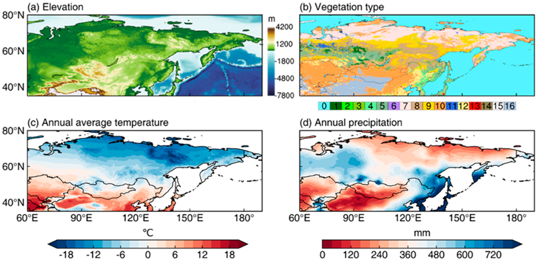
3.1. Climate and Vegetation in the MHA

The topography in the MHA is high in the southwest and low in the north and east, with both plateaus and deserts (Figure 1a). The MHA includes 17 major land cover types. The vegetation types in the central region at approximately 60°N are the most abundant, mainly mixed forest and evergreen needleleaf forest (Figure 1b). The high-latitude region is composed of a large number of open shrublands. Grassland and sparse vegetation are the main vegetation types in the southwestern MHA, including the Mongolian Plateau and part of the Tibetan Plateau, which have high altitudes, arid climates, and fragile ecosystems. The difference in vegetation types causes differences in vegetation phenology, and the major climate elements affecting them are also different.
Most inland areas of the MHA have a temperate continental climate. Its north has a polar climate, and its southeast coastal area has a monsoon climate. The annual average temperature increases from the northeast to the southwest, with the lowest temperature in Central and Eastern Siberia, where the annual average temperature is mostly below −8 °C (Figure 1c). Influenced by the monsoon and topography, the average annual precipitation in the southeast coastal areas is more than 800 mm (Figure 1d). For the central part of the MHA, from the West Siberian plain, through the Balkhash Lake area of the Central Siberian Plateau to the southern part of the Eastern Siberian mountains, the average annual precipitation can reach more than 400 mm. For the far inland regions of Kazakhstan, Xinjiang, China and the eastern part of the Mongolian Plateau, the annual precipitation is less than 200 mm. As a result, persistent droughts often occur in these inland regions [45].
The vegetation growth in the central part of the MHA is the most vigorous, with the annual average LAIs reaching more than 2 m2 m−2 (Figure 2a), while the annual average LAIs in the southwest and high latitudes of the MHA are less than 1 m2 m−2. The pattern of LAI interannual variation is similar to that of the mean LAI (Figure 2b), and the vegetation changes in the Central Siberian Plateau to the west of Lake Baikal and the coasts of the Sea of Japan are the most obvious. The vegetation types in these regions are mainly mixed forest, deciduous broadleaf forest, and evergreen needleleaf forest. The vegetation in most areas of the MHA shows a significant increasing trend in the past 39 years. The high latitudes show the most significant trends, while vegetation degradation occurred to the west of Lake Baikal and the coasts of the Sea of Japan.

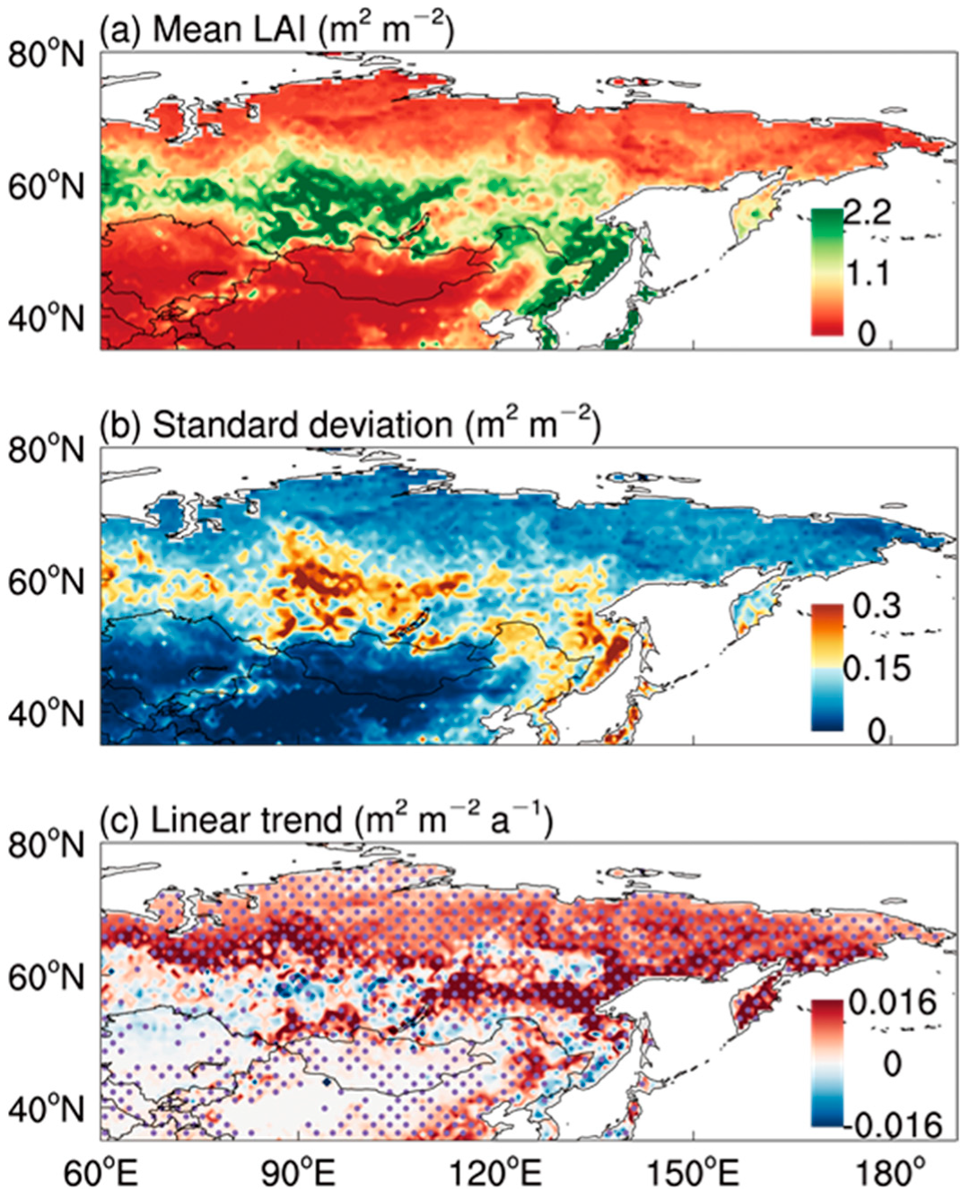
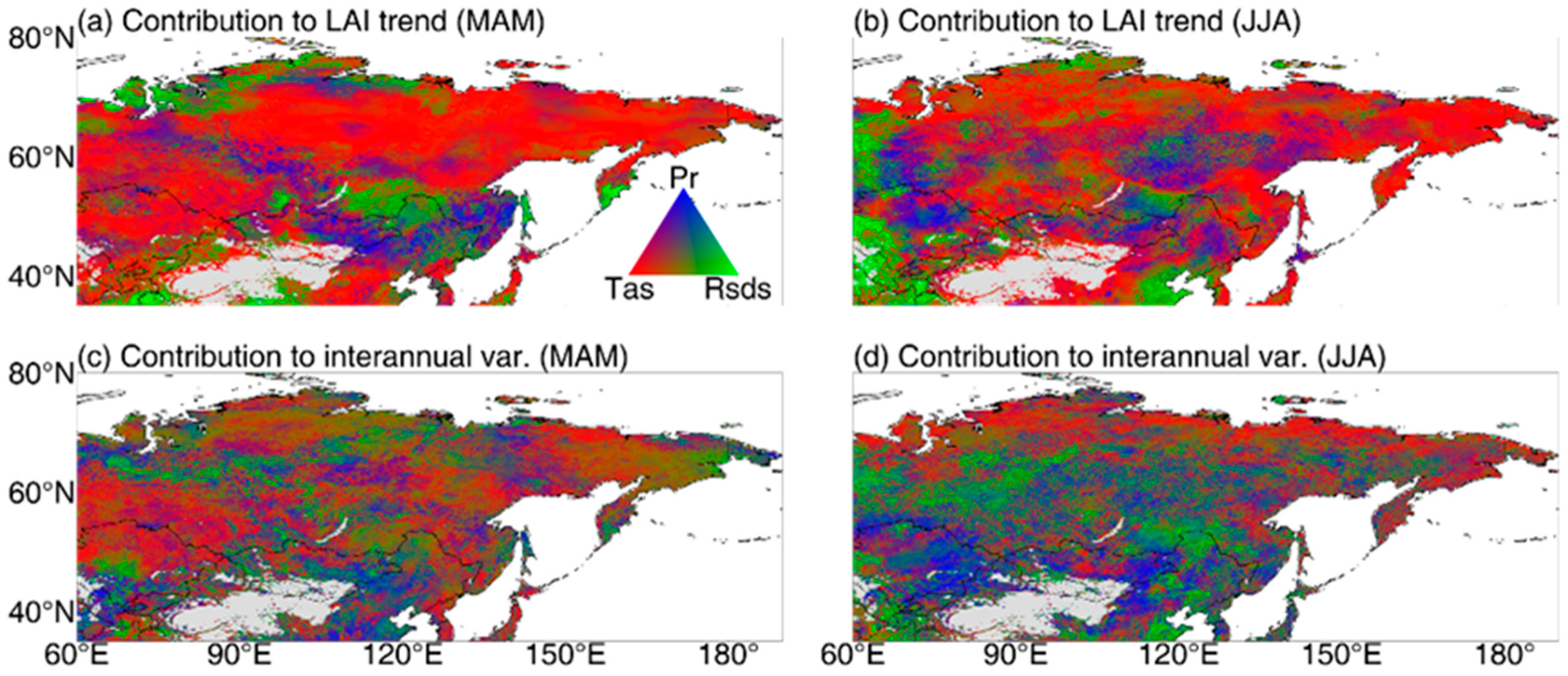
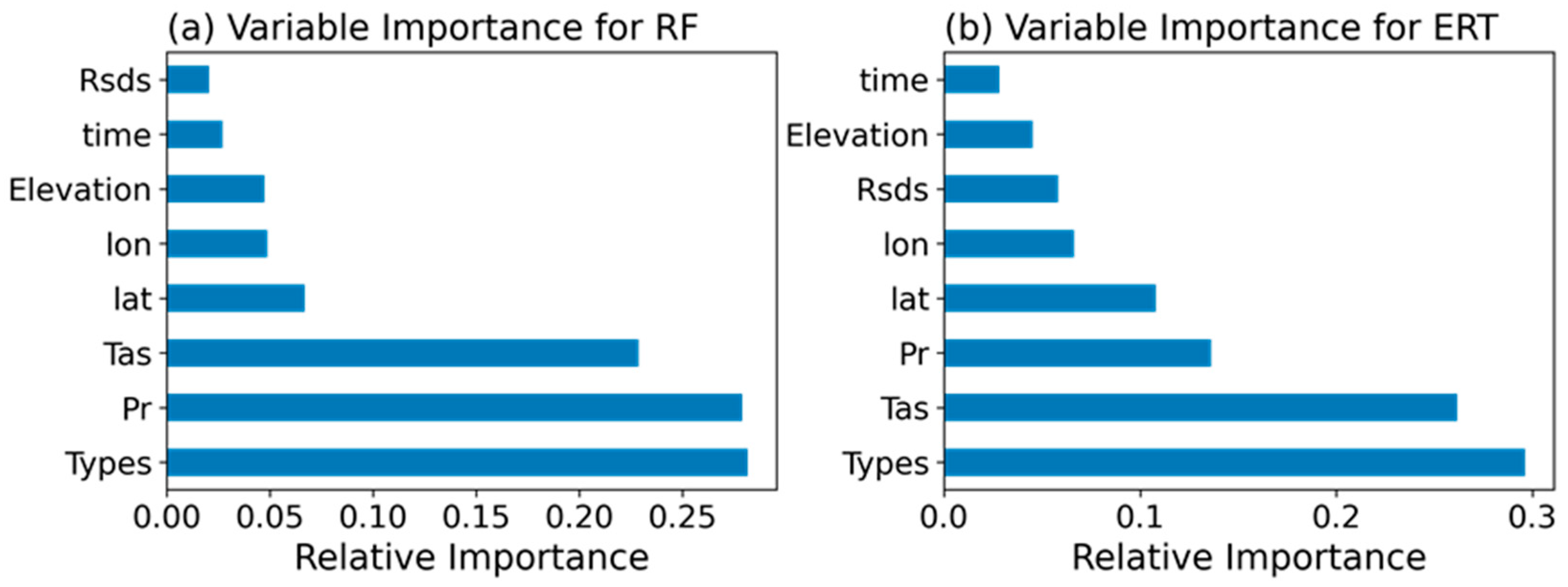
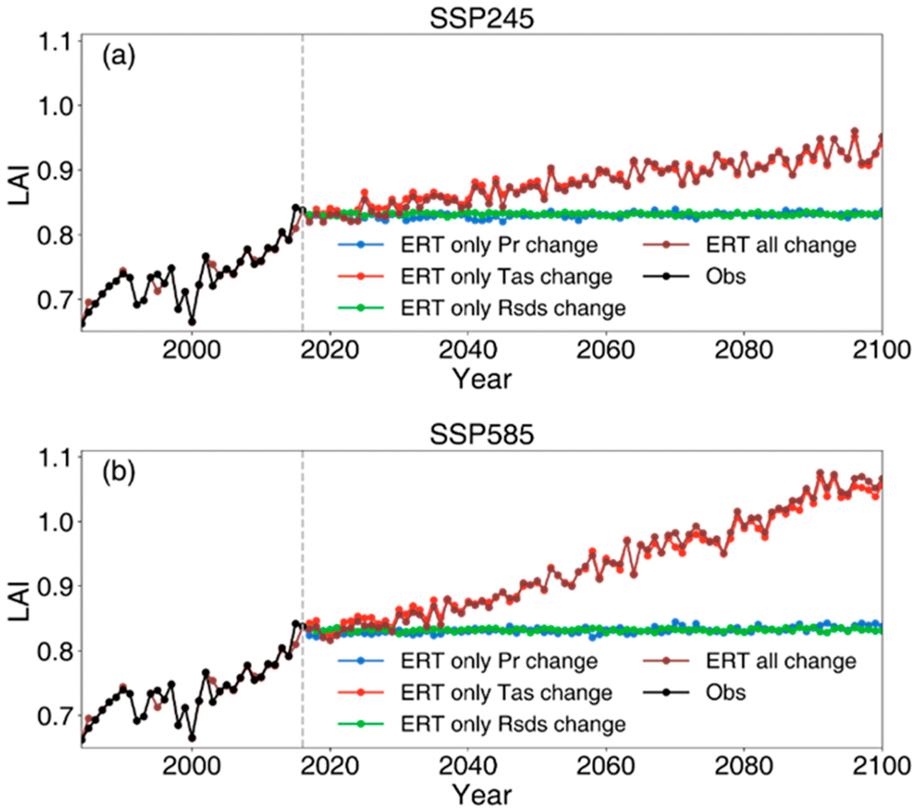
3.2. Climate Elements Affecting the Trend and Interannual Variation of LAI

Figure 3 shows the relative contributions of the three climate elements to the linear trend and interannual variability of LAI in 1984–2016. The results are shown for spring (March–May) and summer (June–August), the two main periods of the growing season, separately. The calculations of the trend and interannual variability are for the averages of spring or summer. For most of the MHA, Tas contributes most to the long-term trend of LAI in both spring and summer, especially in high latitudes where the warming trends are the strongest (Figure 3a–b). This is consistent with previous findings (e.g., Zhou et al. [9]). For the interannual variations of LAI, the relative contributions of Tas are smaller while Pr and Rsds have more contributions (Figure 3c–d). This is more evident in summer, when Rsds is the most important factor for most areas. In the semiarid areas around the Taklamakan Desert and Gobi Desert, Pr is the most important contributor to the interannual variation of summer LAI. Tas is still the most important contributor for most areas in spring and for the high latitudes in summer.

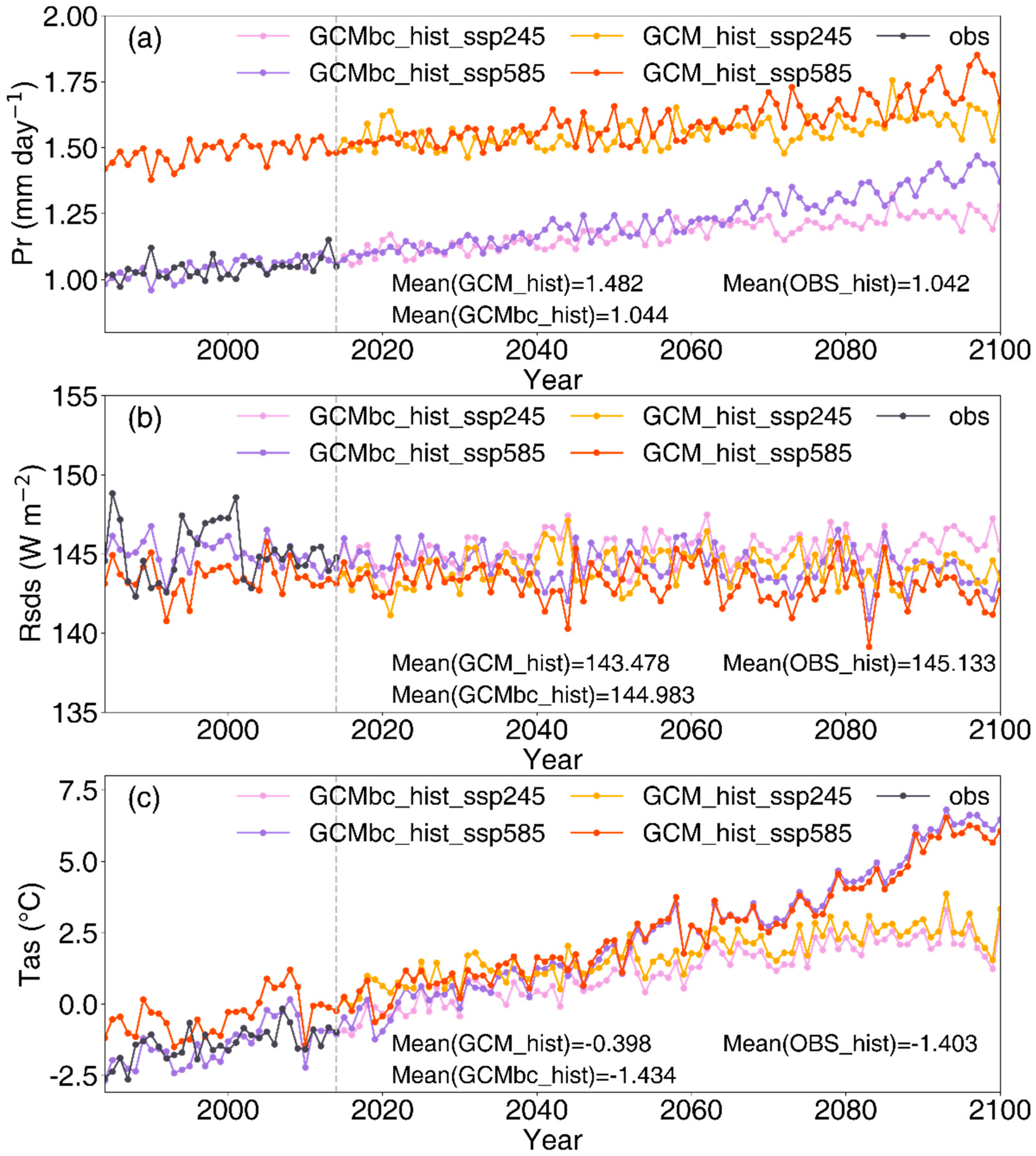
3.3. Bias Correction for CMIP6 Data

As described in Section 2.4, we use the monthly Pr and Tas data from CRU, as well as the ISCCP-FH Rsds in the historical period (1984–2014), to calibrate the detrended monthly data from the MPI-ESM1-2-HR model. The MME data from 17 CMIP6 models provide future (2015–2100) long-term climate changes relative to the historical period. Figure 4 shows the model results for historical and future simulations before and after bias correction. In the historical period, the MPI-ESM1-2-HR model significantly overestimates Pr and Tas and underestimates Rsds. After bias correction, the differences in mean values between the model and observations are greatly reduced. Pr and Tas show increasing trends in the MHA both before and after bias correction, and the trends under the SSP5-8.5 scenario are larger than those under the SSP2-4.5 scenario, especially for Tas. According to the bias-corrected model data, the regional mean Tas under SSP2-4.5 (SSP5-8.5) will increase by nearly 3 °C (7 °C) during 2015–2100. Under both scenarios, the mean Tas values will soon change from below 0 °C in the historical period to above 0 °C in the near future. Perennial snow melting in high-latitude areas will lead to more drastic changes in climate, LAI, and even vegetation types. The long-term trend of Rsds is not significant, and the Rsds under SSP5-8.5 is slightly lower than that under SSP2-4.5.

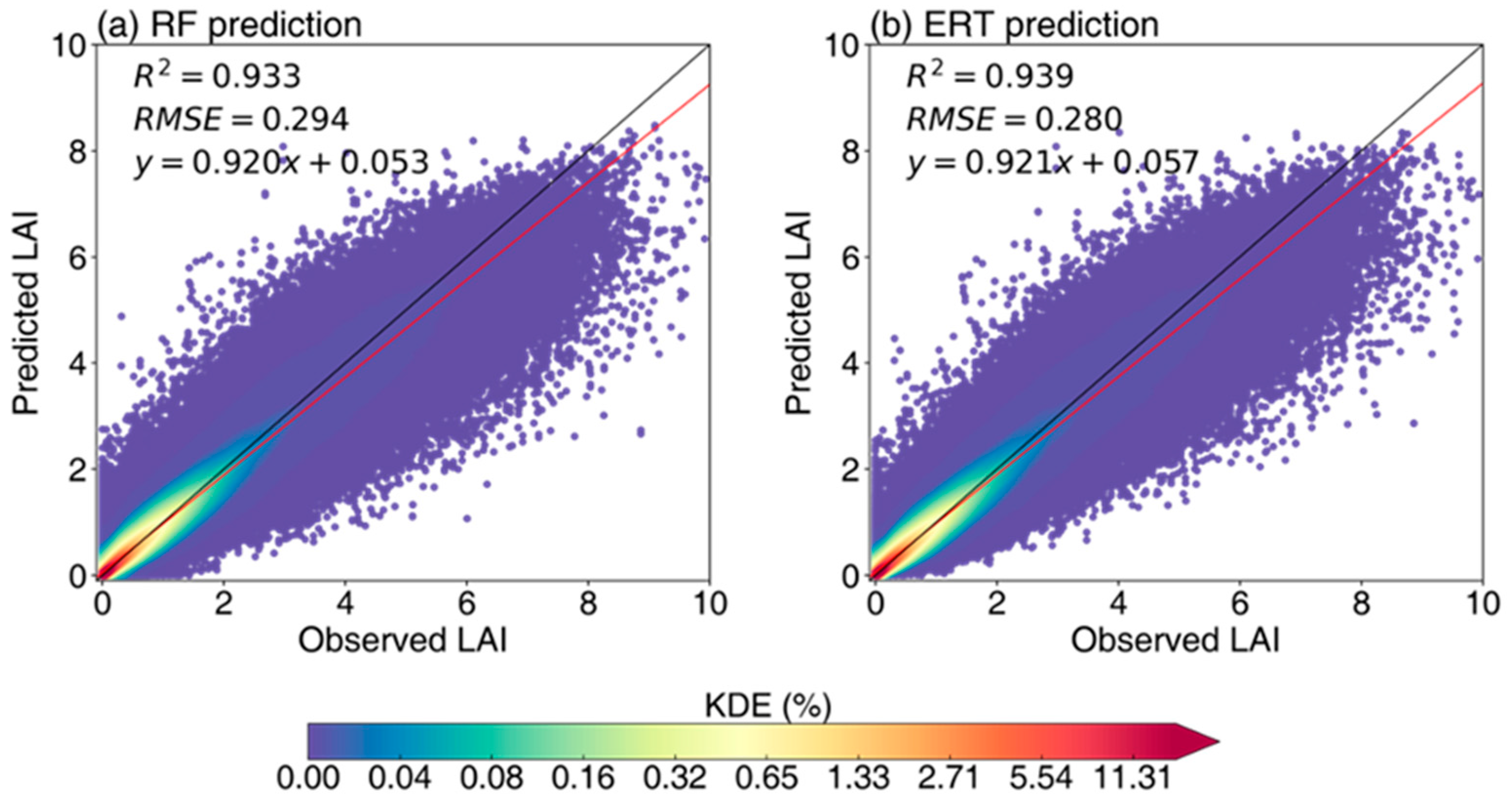
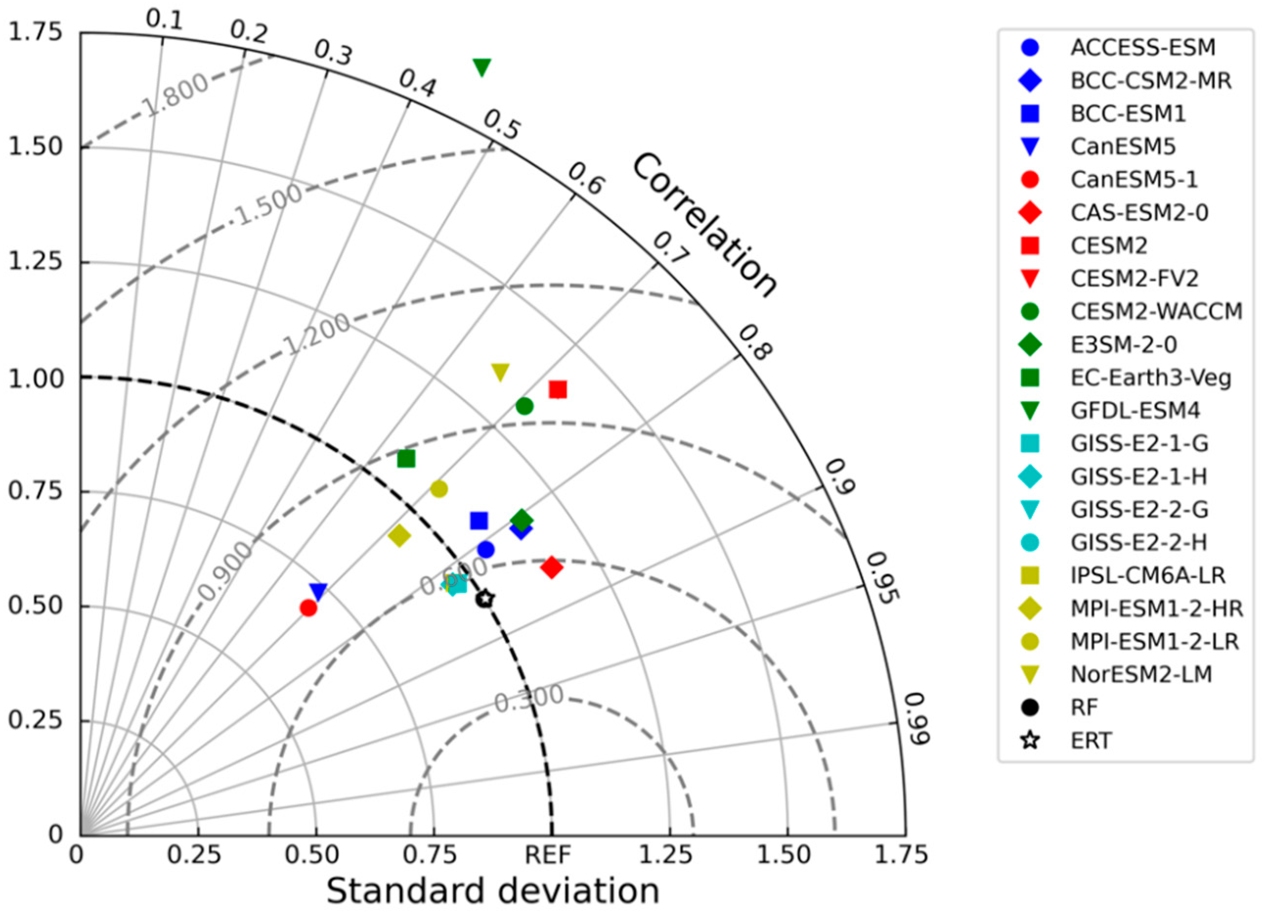
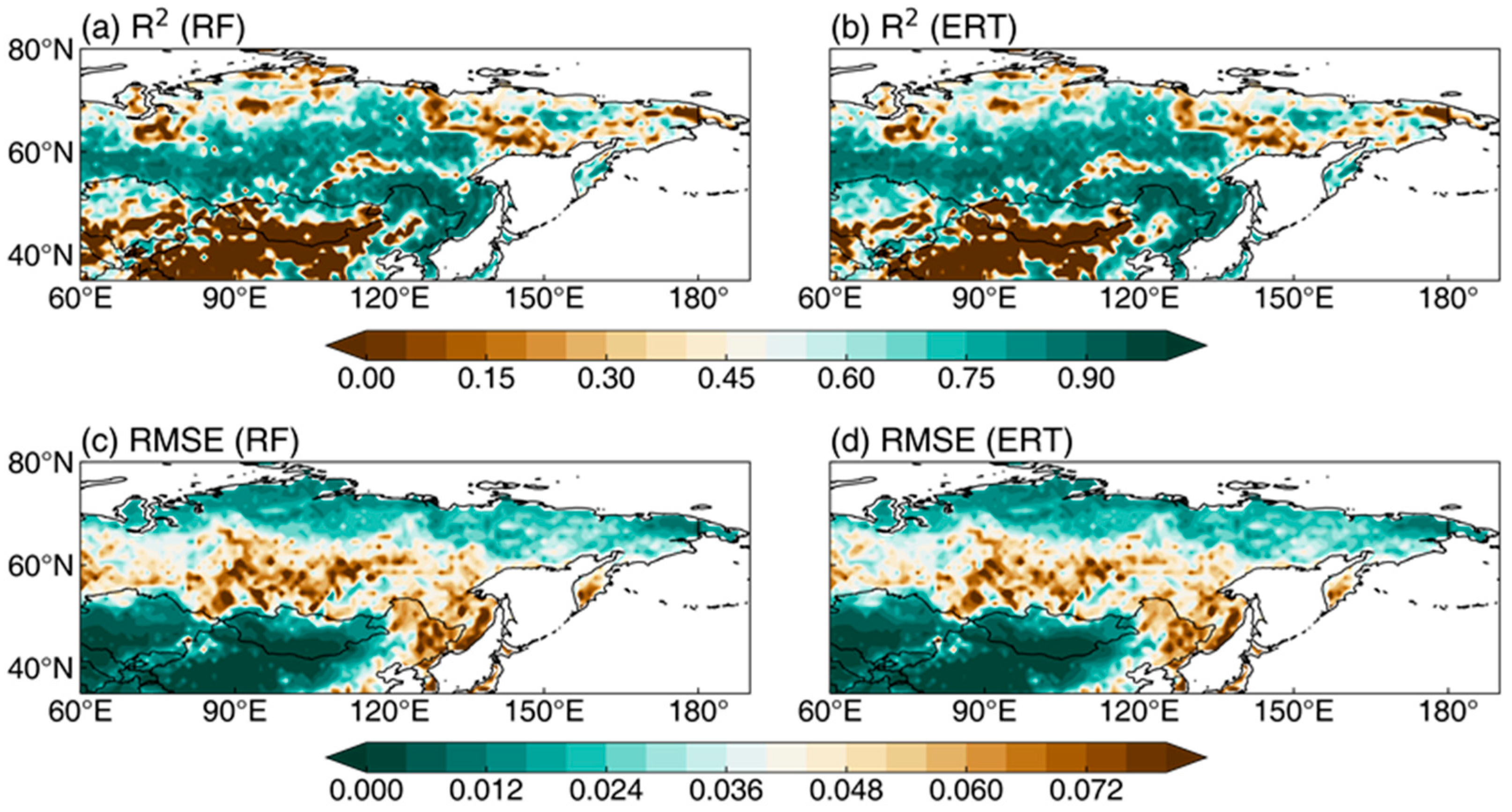
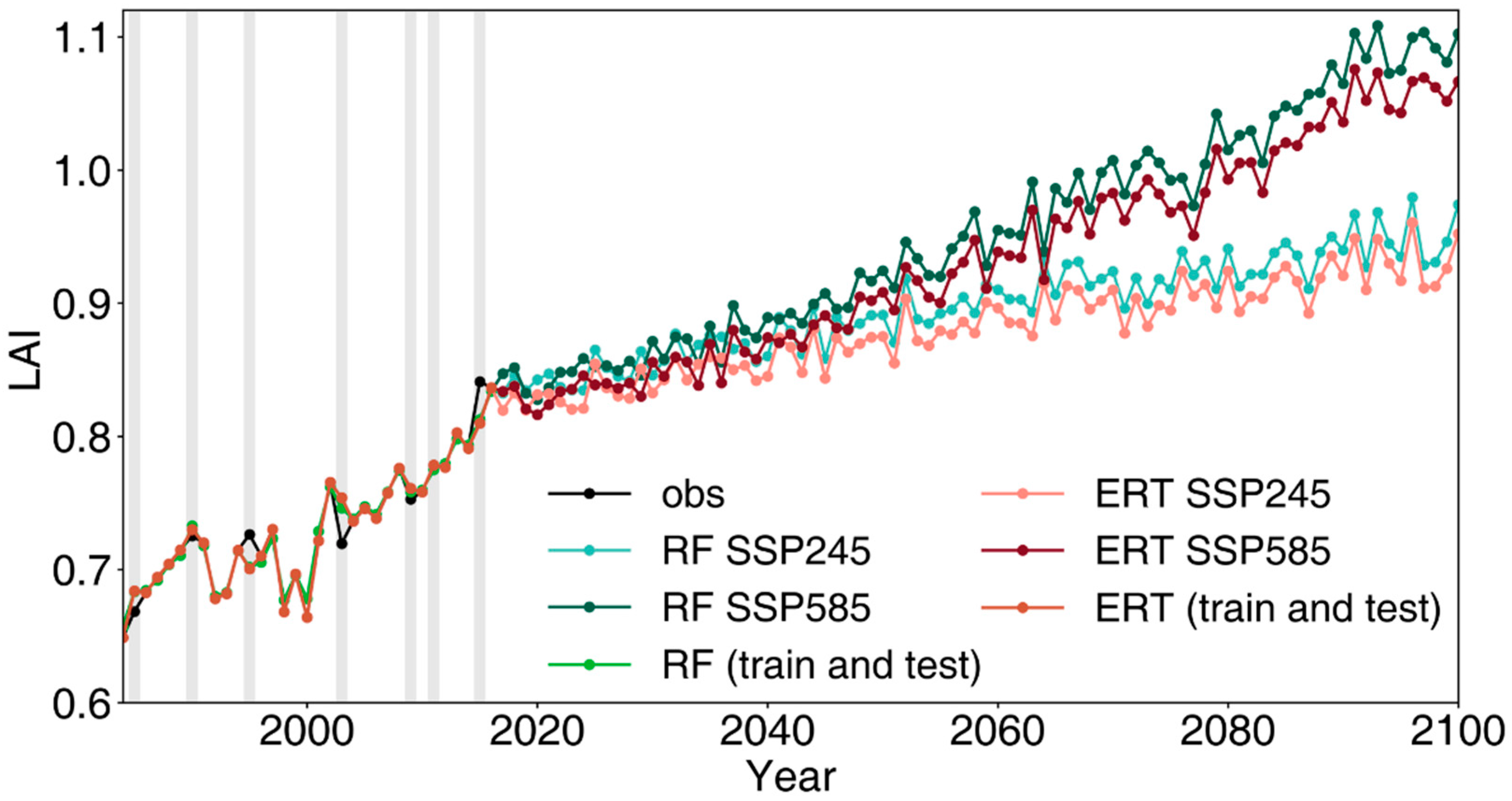
3.4. Evaluation of Machine Learning Models

We used three climate elements, Pr, Tas and Rsds, as well as five background factors, elevation, vegetation type, latitude, longitude, and time, to predict future LAI. The results of cross validation from two prediction models, RF and ERT, are shown in Figure 5. Both models show high determination coefficients (R2) of over 0.93 and low RMSEs of less than 0.3, but both models underestimate the high LAI values. The LAI has the highest density at 0–2.5 m2 m−2, consistent with Figure 2a. The ERT model shows slightly better results than the RF model.
To compare the performance of the machine learning models with those of the CMIP6 models, we show the 1984–2016 predicted annual LAI from 20 CMIP6 models and the two machine learning models (Figure 6). The machine learning models show superior performances compared with all 20 CMIP6 models.
The values of the predictors that are not selected in bootstrap sampling are randomly disturbed, and the difference between the forecast value and the actual observed value is used to determine the importance of the predictors. Figure 7 shows the relative importance of the predictors for prediction in the two models. The vegetation type (Type), Pr and Tas are the most important predictors in the two models. However, Pr is more important than Tas in the RF model, while the reverse is true in the ERT model. The contribution of vegetation type in the models can reach nearly 30%, and different vegetation types have great differences in LAI variability. In our prediction model, the vegetation types remain unchanged, which may have some impact on the long-term LAI predictions.
Figure 8 shows the R2 and RMSE of the two models for the test set. The two models show similar patterns in both R2 and RMSE. R2 has high values in the high-latitude area north of the Mongolia Plateau and the coastal zone where LAI is high, and it has very low values in the mid-latitude dry regions where the vegetation is sparse. RMSE shows a different pattern from that of R2, with higher (lower) values in regions with high (low) LAI. The RMSE in the whole region is mostly below a low value of 0.08 m2 m−2, demonstrating the good performance of the models. The areas with R2 < 0.3 are not included in the subsequent analysis.

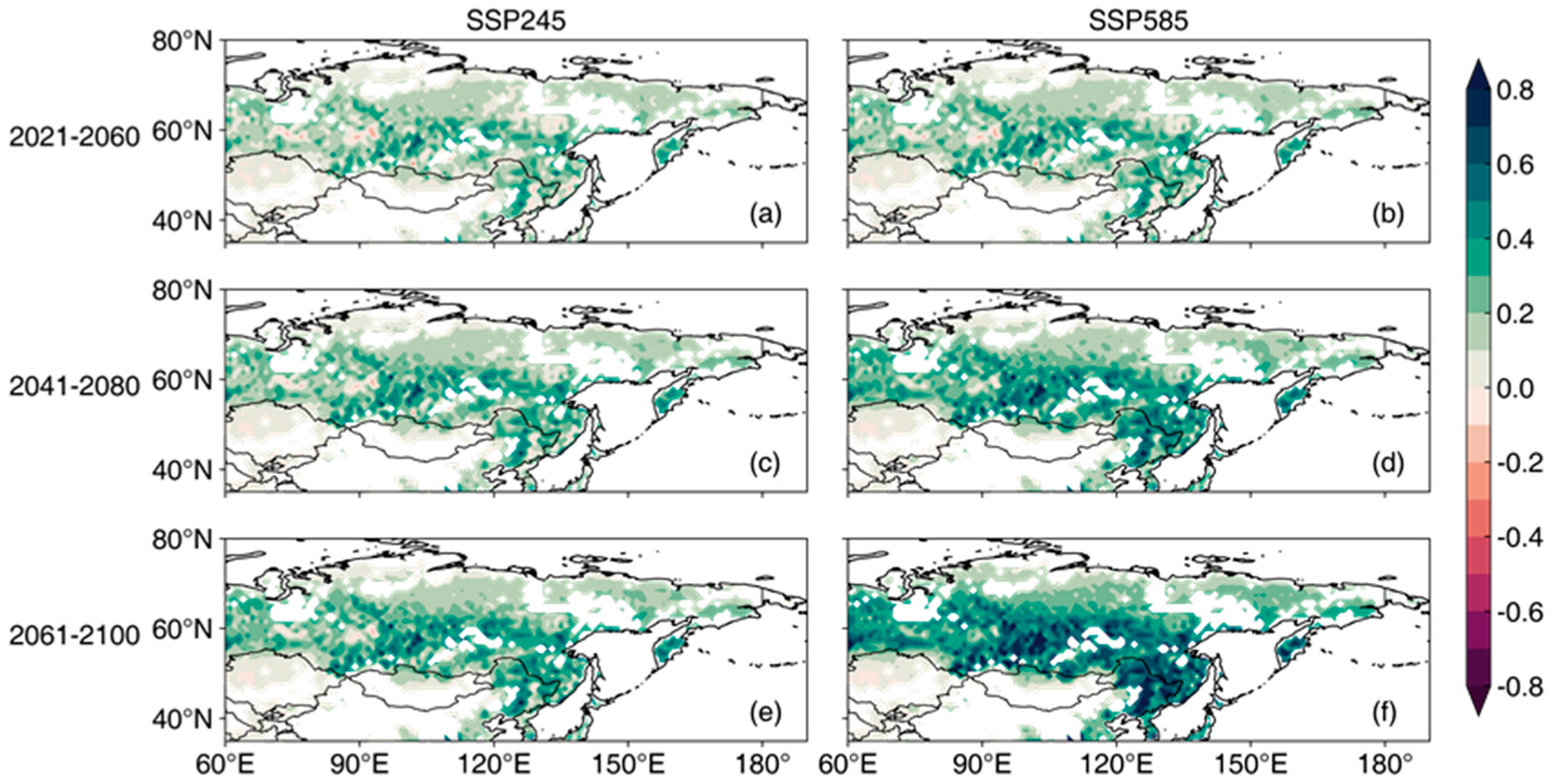
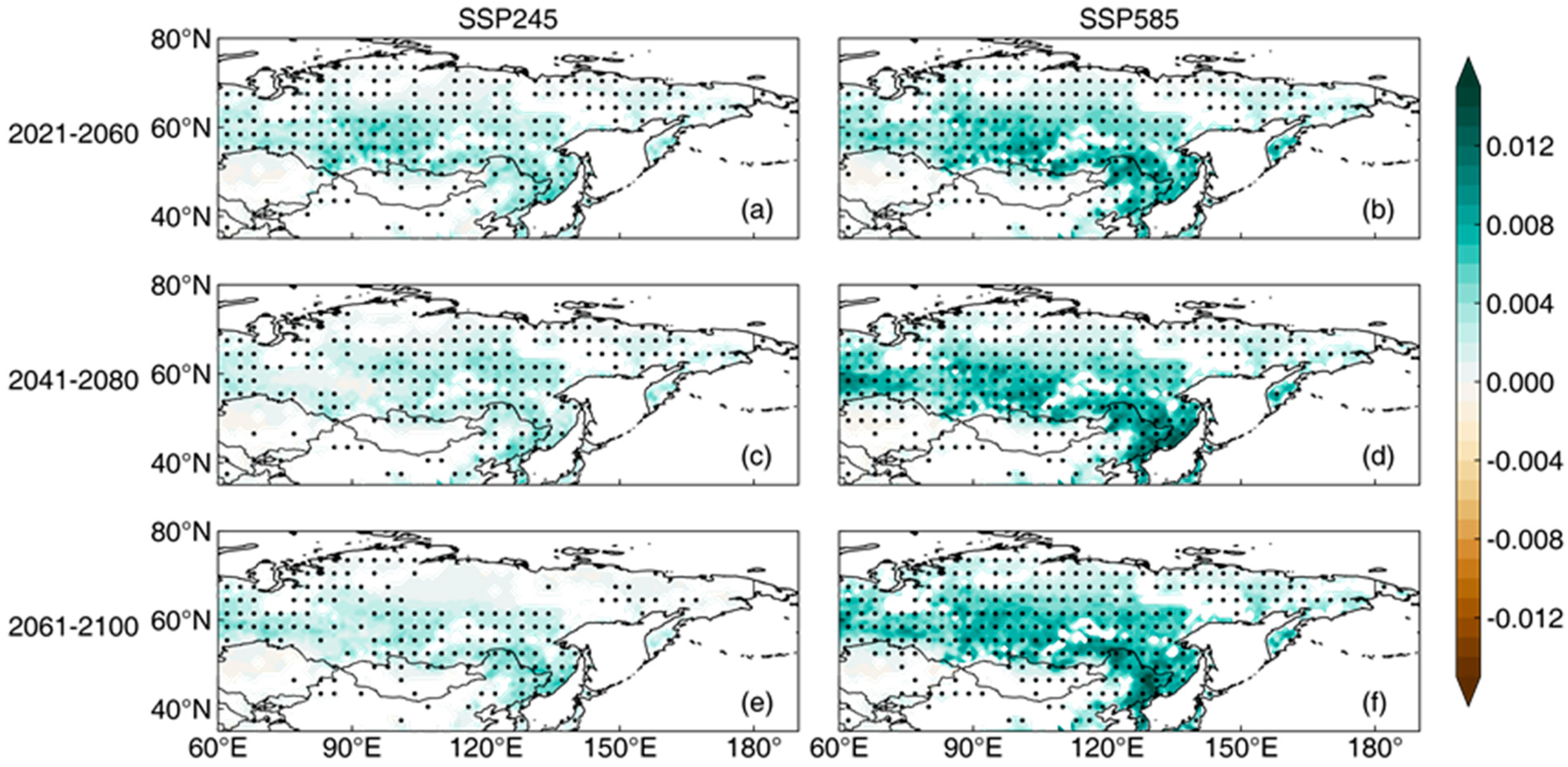
3.5. Projection of Future Vegetation

Figure 9 shows the historical and future LAI produced by the machine learning models RF and ERT according to the observed (1982–2020) and calibrated CMIP6 (2021–2100) climate elements, as well as some background factors. In the historical period, the two models are both very close to the observations during the training periods; the biases are larger in test years (vertical bars), but the interannual to decadal variabilities are properly reproduced. Under the two future scenarios, the two models both show significant increasing trends in the regional average LAI. The increasing trends are stronger under the SSP5-8.5 scenario than under the SSP2-4.5 scenario, and the RF model predicts stronger increases than the ERT model. Because the ERT model has slightly better performance than the RF model (Figure 5), the prediction results of the ERT model are used for subsequent analysis. By the end of the 21st century, the ERT-predicted average annual LAI under SSP2-4.5 and SSP5-8.5 will increase by approximately 0.1 m2/m2 and 0.24 m2/m2, respectively, compared with 2016. Note also that under SSP5-8.5, the speed of LAI increase slows down at the end of the 21st century, consistent with the slowdown of the warming trend.
The regression analysis in Figure 3 shows that Tas is most important for the long-term trend of LAI over most regions of the MHA. To confirm this result, we keep two of the three climate elements (Tas, Pr, and Rsds) constant as the values of 2016 in the ERT model predictions and see how they may affect the projection of future LAI (Figure 10). When only Pr or Rsds changes (blue and green lines), the future LAI does not have an obvious trend. When only Tas changes, the LAI (red line) approaches that predicted when all the climate elements change (brown line). This confirms that the vegetation growth in the MHA is mainly driven by Tas. Note that the curve of only Tas changes and that of all change are not completely the same. By the end of the 21st century, the LAI values from all change are higher than those of only Tas changes, especially under the SSP5-8.5 scenario. This indicates the synergistic effect of Pr, Rsds and Tas on vegetation growth in the future.
We divide the future period of 2021–2100 into three overlapping 40-year periods (2021–2060, 2041–2080, 2061–2100) and calculate their LAI differences with the historical period (1982–2020). Spatially, the LAI in the MHA will be increasing in almost the whole region (Figure 11), and weak vegetation degradation will only occur in a few small areas. As shown in Figure 9, the difference in LAI changes between the SSP2-4.5 and SSP5-8.5 scenarios grows with time, with little difference in 2021–2060, but the differences are evident in 2061–2100. The regions with the strongest LAI increase are at approximately 60°N from northern Kazakhstan to northeast China, similar to the regions with the highest LAI (Figure 2a). The LAI of the MHA is projected to have a largely constant increasing trend from 2021 to 2100, and the growth rate is higher under the SSP5-8.5 scenario than under the SSP2-4.5 scenario (Figure 12). The regions with the fastest LAI growth are basically the regions with the highest LAI.
The mean seasonal cycles of the MHA under future scenarios are similar to those in the historical period, but the LAI values are higher (Figure 13). The largest increases are in spring and summer. As shown in Figure 11 and Figure 12, the LAI values are generally higher under SSP5-8.5 than under SSP2-4.5 for all future periods (2021–2100), except in winter months. The lower winter LAI values during historical periods are probably related to the inconsistency of the GLOBMAP LAI before and after 2000 (based on AVHRR and MODIS data, respectively) and still have uncertainties. The LAI differences between SSP5-8.5 and SSP2-4.5 and between different periods of the same scenario are relatively small in July–August, probably because the high temperature inhibits vegetation growth [14].

4. Discussion

This study used calibrated CMIP6 model data and machine learning methods to project future vegetation changes in the MHA. Some limitations of the study should be noted. Anthropogenic land use and land cover change have contributed greatly to LAI changes in some regions, for example, the reforestation in northern China [46,47]. Their effects are assumed to be constant in this study but this may not be true. Failure to take such factors into account could lead to biases in model training and the estimation of future LAI. The CO2 fertilization effect is another important factor that is not considered. It has a dominant effect on the greening of tropical vegetation, but its influences are relatively minor for the MHA [48]. Moreover, LAI data derived from satellite data have issues of spatiotemporal discontinuity and saturation for dense vegetation, which may affect model training and vegetation prediction. Future studies should examine these uncertainties by using other vegetation indexes (such as solar-induced chlorophyll fluorescence, SIF).
In this study, the RF and ERT models are used because they have fast speed and good fitting abilities and are able to consider nonlinear relationships. One of the limitations of the models is that they can only consider the simultaneous climate-vegetation relationship and do not consider the memory and lagged response of vegetation to climate variations. Some machine learning models, such as LSTM, have memory stores but have high computational costs. The lagged response of vegetation to climate should be explored in future studies. In addition, the RF and ERT models have limited ability to predict extreme values, which may affect the accuracy of their projected vegetation extremes. Because this study focuses on the evolution of mean vegetation, we consider that this limitation should have little influence on the results of this study.
Hernanz et al. [49] showed that machine learning models have limitations in downscaling or projecting future conditions based on past observations, i.e., extrapolation issues. We tested using 1982-2000 as the training period and 2001-2020 as the testing period. The biases are larger than using randomly selected training sets. However, the GLOBMAP LAI is based on AVHRR (MODIS) before (after) 2000, and the biases could also come from the discontinuity of the LAI dataset. The limitations of ML models in extrapolating future scenarios should be paid more attention in future studies. Some emerging physics-constrained ML methods may be a possible way to alleviate these extrapolation problems [50].

5. Conclusions

This study analyzes the characteristics of LAI changes in the MHA over the past 39 years and investigates the relationship between vegetation and climate elements. Two LAI prediction models are built using machine learning methods and are validated. The CMIP6 data for the SSP2-4.5 and SSP5-8.5 scenarios are bias corrected and used by the prediction models to predict the LAI in the future (2021–2100). The long-term increasing trends of vegetation since 1982 in most parts of the MHA are found to be caused by global warming. However, precipitation and radiation also play important roles in the interannual variation of LAI, especially in summer. The vegetation type is a crucial factor in the prediction models. Consistent with previous studies, the LAIs predicted by the two models both show significant increasing trends in most parts of the MHA in the future, and the trends are stronger under the high emission scenario of SSP5-8.5. The regions with the fastest LAI growth are similar to the regions with the highest LAI. The growth of vegetation slows down at the end of the 21st century under the SSP5-8.5 scenario because of the high temperature. The LAI differences between SSP5-8.5 and SSP2-4.5 and between different periods of the same scenario are relatively small in July–August compared with other warm season months, probably because the high temperature inhibits vegetation growth. This study provides a reference for future ecosystem and environmental changes under global climate change.

Author Contributions

Conceptualization, J.W., X.L. and B.Z.; methodology, J.W. and X.L.; software, X.L.; formal analysis, X.L. and J.W.; resources, J.W. and B.Z.; writing—original draft preparation, J.W., X.L.; writing—review and editing, B.Z.; funding acquisition, B.Z. and J.W. All authors have read and agreed to the published version of the manuscript.

Funding

This research was funded by the National Science Foundation of China under grant 41991285.

Data Availability Statement

The data and code for the research are available at https://zenodo.org/record/7865508 (accessed on 15 May 2023).

Acknowledgments

We thank Ye Pu for plotting a figure and Huiming Wang for typesetting the manuscript.

Conflicts of Interest

The authors declare no conflict of interest.

References

  1. Beer, C.; Reichstein, M.; Tomelleri, E.; Ciais, P.; Jung, M.; Carvalhais, N.; Rödenbeck, C.; Arain, M.A.; Baldocchi, D.; Bonan, G.B.; et al. Terrestrial Gross Carbon Dioxide Uptake: Global Distribution and Covariation with Climate. Science 2010, 329, 834–838. [Google Scholar] [CrossRef] [PubMed]
  2. Jones, C.D.; Cox, P.M. On the Significance of Atmospheric CO2 Growth Rate Anomalies in 2002–2003. Geophys. Res. Lett. 2005, 32, L14816. [Google Scholar] [CrossRef]
  3. Piao, S.; Nan, H.; Huntingford, C.; Ciais, P.; Friedlingstein, P.; Sitch, S.; Peng, S.; Ahlström, A.; Canadell, J.G.; Cong, N.; et al. Evidence for a Weakening Relationship between Interannual Temperature Variability and Northern Vegetation Activity. Nat. Commun. 2014, 5, 5018. [Google Scholar] [CrossRef]
  4. Nemani, R.R.; Keeling, C.D.; Hashimoto, H.; Jolly, W.M.; Piper, S.C.; Tucker, C.J.; Myneni, R.B.; Running, S.W. Climate-Driven Increases in Global Terrestrial Net Primary Production from 1982 to 1999. Science 2003, 300, 1560–1563. [Google Scholar] [CrossRef]
  5. Craine, J.M.; Nippert, J.B.; Elmore, A.J.; Skibbe, A.M.; Hutchinson, S.L.; Brunsell, N.A. Timing of Climate Variability and Grassland Productivity. Proc. Natl. Acad. Sci. USA 2012, 109, 3401–3405. [Google Scholar] [CrossRef]
  6. Seddon, A.W.R.; Macias-Fauria, M.; Long, P.R.; Benz, D.; Willis, K.J. Sensitivity of Global Terrestrial Ecosystems to Climate Variability. Nature 2016, 531, 229–232. [Google Scholar] [CrossRef]
  7. Zhou, L.; Tian, Y.; Myneni, R.B.; Ciais, P.; Saatchi, S.; Liu, Y.Y.; Piao, S.; Chen, H.; Vermote, E.F.; Song, C.; et al. Widespread Decline of Congo Rainforest Greenness in the Past Decade. Nature 2014, 509, 86–90. [Google Scholar] [CrossRef]
  8. De Andrade, A.M.; Michel, R.F.M.; Bremer, U.F.; Schaefer, C.E.G.R.; Simões, J.C. Relationship between Solar Radiation and Surface Distribution of Vegetation in Fildes Peninsula and Ardley Island, Maritime Antarctica. Int. J. Remote Sens. 2018, 39, 2238–2254. [Google Scholar] [CrossRef]
  9. Zhou, L.; Tucker, C.J.; Kaufmann, R.K.; Slayback, D.; Shabanov, N.V.; Myneni, R.B. Variations in Northern Vegetation Activity Inferred from Satellite Data of Vegetation Index during 1981 to 1999. J. Geophys. Res. Atmos. 2001, 106, 20069–20083. [Google Scholar] [CrossRef]
  10. Fensholt, R.; Langanke, T.; Rasmussen, K.; Reenberg, A.; Prince, S.D.; Tucker, C.; Scholes, R.J.; Le, Q.B.; Bondeau, A.; Eastman, R.; et al. Greenness in Semi-Arid Areas across the Globe 1981–2007—An Earth Observing Satellite Based Analysis of Trends and Drivers. Remote Sens. Environ. 2012, 121, 144–158. [Google Scholar] [CrossRef]
  11. Cong, N.; Wang, T.; Nan, H.; Ma, Y.; Wang, X.; Myneni, R.B.; Piao, S. Changes in Satellite-Derived Spring Vegetation Green-up Date and Its Linkage to Climate in China from 1982 to 2010: A Multimethod Analysis. Glob. Chang. Biol. 2013, 19, 881–891. [Google Scholar] [CrossRef]
  12. Zelikova, T.J.; Williams, D.G.; Hoenigman, R.; Blumenthal, D.M.; Morgan, J.A.; Pendall, E. Seasonality of Soil Moisture Mediates Responses of Ecosystem Phenology to Elevated CO2 and Warming in a Semi-Arid Grassland. J. Ecol. 2015, 103, 1119–1130. [Google Scholar] [CrossRef]
  13. Garonna, I.; de Jong, R.; de Wit, A.J.W.; Mücher, C.A.; Schmid, B.; Schaepman, M.E. Strong Contribution of Autumn Phenology to Changes in Satellite-Derived Growing Season Length Estimates across Europe (1982–2011). Glob. Chang. Biol. 2014, 20, 3457–3470. [Google Scholar] [CrossRef] [PubMed]
  14. Zhang, Y.; Piao, S.; Sun, Y.; Rogers, B.M.; Li, X.; Lian, X.; Liu, Z.; Chen, A.; Peñuelas, J. Future Reversal of Warming-Enhanced Vegetation Productivity in the Northern Hemisphere. Nat. Clim. Chang. 2022, 12, 581–586. [Google Scholar] [CrossRef]
  15. Shinoda, M.; Nandintsetseg, B. Soil Moisture and Vegetation Memories in a Cold, Arid Climate. Glob. Planet. Change 2011, 79, 110–117. [Google Scholar] [CrossRef]
  16. Lin, Y.; Xin, X.; Zhang, H.; Wang, X. The Implications of Serial Correlation and Time-Lag Effects for the Impact Study of Climate Change on Vegetation Dynamics—A Case Study with Hulunber Meadow Steppe, Inner Mongolia. Int. J. Remote Sens. 2015, 36, 5031–5044. [Google Scholar] [CrossRef]
  17. Mohammat, A.; Wang, X.; Xu, X.; Peng, L.; Yang, Y.; Zhang, X.; Myneni, R.B.; Piao, S. Drought and Spring Cooling Induced Recent Decrease in Vegetation Growth in Inner Asia. Agric. For. Meteorol. 2013, 178–179, 21–30. [Google Scholar] [CrossRef]
  18. Reichstein, M.; Ciais, P.; Papale, D.; Valentini, R.; Running, S.; Viovy, N.; Cramer, W.; Granier, A.; Ogée, J.; Allard, V.; et al. Reduction of Ecosystem Productivity and Respiration during the European Summer 2003 Climate Anomaly: A Joint Flux Tower, Remote Sensing and Modelling Analysis. Glob. Chang. Biol. 2007, 13, 634–651. [Google Scholar] [CrossRef]
  19. Iwasaki, H. NDVI Prediction over Mongolian Grassland Using GSMaP Precipitation Data and JRA-25/JCDAS Temperature Data. J. Arid Environ. 2009, 73, 557–562. [Google Scholar] [CrossRef]
  20. Wang, S.; Huang, G.H.; Huang, W.; Fan, Y.R.; Li, Z. A Fractional Factorial Probabilistic Collocation Method for Uncertainty Propagation of Hydrologic Model Parameters in a Reduced Dimensional Space. J. Hydrol. 2015, 529, 1129–1146. [Google Scholar] [CrossRef]
  21. Huang, S.; Ming, B.; Huang, Q.; Leng, G.; Hou, B. A Case Study on a Combination NDVI Forecasting Model Based on the Entropy Weight Method. Water Resour. Manag. 2017, 31, 3667–3681. [Google Scholar] [CrossRef]
  22. Yuan, W.; Wu, S.-Y.; Hou, S.; Xu, Z.; Pang, H.; Lu, H. Projecting Future Vegetation Change for Northeast China Using CMIP6 Model. Remote Sens. 2021, 13, 3531. [Google Scholar] [CrossRef]
  23. Liu, B.; Tang, Q.; Zhou, Y.; Zeng, T.; Zhou, T. The Sensitivity of Vegetation Dynamics to Climate Change across the Tibetan Plateau. Atmosphere 2022, 13, 1112. [Google Scholar] [CrossRef]
  24. Zhou, Z.; Ding, Y.; Shi, H.; Cai, H.; Fu, Q.; Liu, S.; Li, T. Analysis and Prediction of Vegetation Dynamic Changes in China: Past, Present and Future. Ecol. Indic. 2020, 117, 106642. [Google Scholar] [CrossRef]
  25. Parton, W.J.; Scurlock, J.M.O.; Ojima, D.S.; Gilmanov, T.G.; Scholes, R.J.; Schimel, D.S.; Kirchner, T.; Menaut, J.-C.; Seastedt, T.; Garcia Moya, E.; et al. Observations and Modeling of Biomass and Soil Organic Matter Dynamics for the Grassland Biome Worldwide. Global Biogeochem. Cycles 1993, 7, 785–809. [Google Scholar] [CrossRef]
  26. McGuire, D.A.; Melillo, J.M.; Kicklighter, D.W.; Pan, Y.; Xiao, X.; Helfrich, J.; Moore, B., III; Vorosmarty, C.J.; Schloss, A.L. Equilibrium Responses of Global Net Primary Production and Carbon Storage to Doubled Atmospheric Carbon Dioxide: Sensitivity to Changes in Vegetation Nitrogen Concentration. Global Biogeochem. Cycles 1997, 11, 173–189. [Google Scholar] [CrossRef]
  27. White, M.A.; Thornton, P.E.; Running, S.W.; Nemani, R.R. Parameterization and sensitivity analysis of the BIOME-BGC terrestirial ecosystem model: Net primary production controls. Earth Interact. 2000, 4, 1–85. [Google Scholar] [CrossRef]
  28. Foley, J.A.; Prentice, I.C.; Ramankutty, N.; Levis, S.; Pollard, D.; Sitch, S.; Haxeltine, A. An integrated biosphere model of land surface processes, terrestrial carbon balance, and vegetation dynamics. Glob. Biogeochem. Cycles 1996, 10, 603–628. [Google Scholar] [CrossRef]
  29. Sitch, S.; Smith, B.; Prentice, I.C.; Arneth, A.; Bondeau, A.; Cramer, W.; Kaplan, J.O.; Levis, S.; Lucht, W.; Sykes, M.T.; et al. Evaluation of ecosystem dynamics, plant geography and terrestrial carbon cycling in the LPJ dynamic global vegetation model. Glob. Chang. Biol. 2003, 9, 161–185. [Google Scholar] [CrossRef]
  30. Chen, Z.; Liu, H.; Xu, C.; Wu, X.; Liang, B.; Cao, J.; Chen, D. Modeling Vegetation Greenness and Its Climate Sensitivity with Deep-Learning Technology. Ecol. Evol. 2021, 11, 7335–7345. [Google Scholar] [CrossRef]
  31. Huang, S.; Chang, J.; Huang, Q.; Chen, Y. Monthly Streamflow Prediction Using Modified EMD-Based Support Vector Machine. J. Hydrol. 2014, 511, 764–775. [Google Scholar] [CrossRef]
  32. Navarro-Racines, C.; Tarapues, J.; Thornton, P.; Jarvis, A.; Ramirez-Villegas, J. High-Resolution and Bias-Corrected CMIP5 Projections for Climate Change Impact Assessments. Sci. Data 2020, 7, 7. [Google Scholar] [CrossRef] [PubMed]
  33. Xu, Z.; Han, Y.; Tam, C.-Y.; Yang, Z.-L.; Fu, C. Bias-Corrected CMIP6 Global Dataset for Dynamical Downscaling of the Historical and Future Climate (1979–2100). Sci. Data 2021, 8, 293. [Google Scholar] [CrossRef] [PubMed]
  34. Nakamura, Y.; Krestov, P.; Omelko, A.; Vladivostok. Russia Bioclimate and Zonal Vegetation in Northeast Asia: First Approximation to an Integrated Study. Phytocoenologia 2007, 37, 443–470. [Google Scholar] [CrossRef]
  35. Lee, J.-Y.; Marotzke, J.; Bala, G.; Cao, L.; Corti, S.; Dunne, J.P.; Engelbrecht, F.; Fischer, E.; Fyfe, J.C.; Jones, C.; et al. Future Global Climate: Scenario-Based Projections and Near-Term Information. In Climate Change 2021: The Physical Science Basis. Contribution of Working Group I to the Sixth Assessment Report of the Intergovernmental Panel on Climate Change; Masson-Delmotte, V.P., Zhai, A., Pirani, S.L., Connors, C., Péan, S., Berger, N., Caud, Y., Chen, L., Goldfarb, M.I., Gomis, M., et al., Eds.; Cambridge University Press: Cambridge, UK, 2021; pp. 553–672. [Google Scholar]
  36. Harris, I.; Osborn, T.J.; Jones, P.; Lister, D. Version 4 of the CRU TS monthly high-resolution gridded multivariate climate dataset. Sci. Data 2020, 7, 109. [Google Scholar] [CrossRef]
  37. Amante, C.; Eakins, B. ETOPO1 1 Arc-Minute Global Relief Model: Procedures, Data Sources and Analysis; NOAA: Boulder, CO, USA, 2009. [Google Scholar] [CrossRef]
  38. Liu, Y.; Liu, R.; Chen, J.M. Retrospective Retrieval of Long-Term Consistent Global Leaf Area Index (1981–2011) from Combined AVHRR and MODIS Data. J. Geophys. Res. Biogeosci. 2012, 117. [Google Scholar] [CrossRef]
  39. Fang, H.; Jiang, C.; Li, W.; Wei, S.; Baret, F.; Chen, J.M.; Garcia-Haro, J.; Liang, S.; Liu, R.; Myneni, R.B.; et al. Characterization and Intercomparison of Global Moderate Resolution Leaf Area Index (LAI) Products: Analysis of Climatologies and Theoretical Uncertainties. J. Geophys. Res. Biogeosci. 2013, 118, 529–548. [Google Scholar] [CrossRef]
  40. Jiang, C.; Ryu, Y.; Fang, H.; Myneni, R.; Claverie, M.; Zhu, Z. Inconsistencies of Interannual Variability and Trends in Long-Term Satellite Leaf Area Index Products. Glob. Chang. Biol. 2017, 23, 4133–4146. [Google Scholar] [CrossRef]
  41. Friedl, M.A.; McIver, D.K.; Hodges, J.C.F.; Zhang, X.Y.; Muchoney, D.; Strahler, A.H.; Woodcock, C.E.; Gopal, S.; Schneider, A.; Cooper, A.; et al. Global Land Cover Mapping from MODIS: Algorithms and Early Results. Remote Sens. Environ. 2002, 83, 287–302. [Google Scholar] [CrossRef]
  42. Zhang, M.; Lin, H.; Long, X.; Cai, Y. Analyzing the Spatiotemporal Pattern and Driving Factors of Wetland Vegetation Changes Using 2000–2019 Time-Series Landsat Data. Sci. Total Environ. 2021, 780, 146615. [Google Scholar] [CrossRef]
  43. Wu, W.-Y.; Lo, M.-H.; Wada, Y.; Famiglietti, J.S.; Reager, J.T.; Yeh, P.J.-F.; Ducharne, A.; Yang, Z.-L. Divergent Effects of Climate Change on Future Groundwater Availability in Key Mid-Latitude Aquifers. Nat. Commun. 2020, 11, 3710. [Google Scholar] [CrossRef]
  44. Wu, Z.; Huang, N.E. Ensemble Empirical Mode Decomposition: A Noise-Assisted Data Analysis Method. Adv. Adapt. Data Anal. 2009, 1, 1–41. [Google Scholar] [CrossRef]
  45. Fernández-Giménez, M.E.; Batkhishig, B.; Batbuyan, B. Cross-Boundary and Cross-Level Dynamics Increase Vulnerability to Severe Winter Disasters (Dzud) in Mongolia. Glob. Environ. Chang. 2012, 22, 836–851. [Google Scholar] [CrossRef]
  46. Tan, M.; Li, X. Does the Green Great Wall Effectively Decrease Dust Storm Intensity in China? A Study Based on NOAA NDVI and Weather Station Data. Land Use Policy 2015, 43, 42–47. [Google Scholar] [CrossRef]
  47. Wei, J.; Jin, Q.; Yang, Z.-L.; Zhou, L. Land–Atmosphere–Aerosol Coupling in North China during 2000–2013. Int. J. Climatol. 2017, 37, 1297–1306. [Google Scholar] [CrossRef]
  48. Zhu, Z.; Piao, S.; Myneni, R.B.; Huang, M.; Zeng, Z.; Canadell, J.G.; Ciais, P.; Sitch, S.; Friedlingstein, P.; Arneth, A.; et al. Greening of the Earth and its drivers. Nat. Clim. Chang. 2016, 6, 791–795. [Google Scholar] [CrossRef]
  49. Hernanz, A.; García-Valero, J.A.; Domínguez, M.; Rodríguez-Camino, E. A critical view on the suitability of machine learning techniques to downscale climate change projections: Illustration for temperature with a toy experiment. Atmos. Sci. Lett. 2022, 23, e1087. [Google Scholar] [CrossRef]
  50. Kashinath, K.; Mustafa, M.; Albert, A.; Wu, J.L.; Jiang, C.; Esmaeilzadeh, S.; Azizzadenesheli, K.; Wang, R.; Chattopadhyay, A.; Singh, A.; et al. Physics-informed machine learning: Case studies for weather and climate modelling. Phil. Trans. Roy Soc. A 2021, 379, 20200093. [Google Scholar] [CrossRef]
Figure 1. Land cover types and climate in the MHA. (a) Topographic map (unit: m), (b) land cover type, (c) annual average surface temperature (unit: °C) and (d) annual total precipitation (unit: mm). Land cover type comes from MODIS land cover type products: 0.Water; 1.Evergreen needleleaf forest; 2. Evergreen broadleaf forest; 3. Deciduous needleleaf forest; 4. Deciduous broadleaf forest; 5. Mixed forest; 6. Closed shrublands; 7. Open shrublands; 8. Woody savannas; 9. Savannas; 10. Grasslands; 11. Permanent Wetland; 12. Croplands; 13. Urban and built-up; 14. Cropland/Natural vegetation mosaics; 15. Snow and ice; 16. Barren or sparsely vegetated.
Remotesensing 15 02648 g001
Figure 2. Spatial distribution of the (a) climatological mean (unit: m2 m−2), (b) standard deviation (unit: m2 m−2) and (c) linear trend (unit: m2 m–2 a–1) of the annual mean LAI from 1982 to 2020 (data from GLOBMAP). Dots highlight areas with trends significant at p < 0.1 level according to the Student’s t test.
Remotesensing 15 02648 g002
Figure 3. Relative contributions of (a,c) spring and (b,d) summer precipitation (Pr; blue), downward shortwave radiation (Rsds; green) and 2 m temperature (Tas; red) to the (a,b) long-term trend and (c,d) interannual variation of LAI in 1984–2016. The trend and interannual variability are for the spring or summer averages of each year. Areas with LAI ≤ 0 are masked.
Remotesensing 15 02648 g003
Figure 4. Original MPI-ESM1-2-HR model (GCM_hist_SSP2-4.5 and GCM_hist_SSP5-8.5) and bias-corrected model (GCMbc_hist_SSP2-4.5 and GCMbc_hist_SSP5-8.5) data in historical (1984–2014) and future (2015–2100) periods under the SSP2-4.5 and SSP5-8.5 scenarios. Observational data from CRU (Tas and Pr) and ISCCP-FH (Rsds) in the historical period are also shown. The vertical line in 2014 separates the historical and future periods. (a) Pr. (b) Rsds. (c) Tas.
Remotesensing 15 02648 g004
Figure 5. Density scatter plots of the relationship between the predicted and observed LAIs from the cross validations by (a) the RF model and (b) the ERT model. Each point represents the monthly mean LAI in one grid cell over the MHA (unit: m2 m−2).
Remotesensing 15 02648 g005
Figure 6. Taylor diagram showing the performance of the predicted 1984–2016 annual LAI from 20 CMIP6 models and the machine learning models (RF and ERT). The symbols for ERT and RF are very close because their results are very similar.
Remotesensing 15 02648 g006
Figure 7. Relative importance of predictors in the (a) RF model and (b) ERT model.
Remotesensing 15 02648 g007
Figure 8. Coefficient of determination (R2; a,b) and root mean square error (RMSE; m2 m−2; c,d) of the predicted LAI from the RF model (a,c) and ERT model (b,d) relative to GLOBMAP LAI for a test set in the historical period (1984–2014).
Remotesensing 15 02648 g008
Figure 9. Interannual variations (1984–2100) of the observation-based (GLOBMAP) and machine learning model (RF and ERT) produced mean LAI in the MHA. The vertical bars show an example of the 20% test years for cross validation.
Remotesensing 15 02648 g009
Figure 10. Interannual variations of LAI in the MHA from ERT predictions and historical observations. See text for details. The vertical line in 2014 separates the historical and future periods. (a) SSP2-4.5. (b) SSP5-8.5.
Remotesensing 15 02648 g010
Figure 11. ERT model projected future mean LAI changes under the SSP2-4.5 and SSP5-8.5 scenarios (2021–2060, 2041–2080, 2061–2100) relative to historical (1982–2020) LAI from GLOBMAP. No value is shown in areas where the ERT model is not reliable (R2 < 0.3 in Figure 8b). (a,c,e) SSP2-4.5. (b,d,f) SSP5-8.5. (a,b) 2021–2060. (c,d) 2041–2080. (e,f) 2061–2100.
Remotesensing 15 02648 g011
Figure 12. (af) Same as Figure 11, but for ERT model projected annual LAI linear trends under the SSP2-4.5 and SSP5-8.5 scenarios for 2021–2060, 2041–2080, and 2061–2100. Dots highlight areas with trends significant at p < 0.1 level according to the Student’s t test. No value is shown in areas where the ERT model is not reliable (R2 < 0.3 in Figure 8b).
Remotesensing 15 02648 g012
Figure 13. Mean seasonal cycle of the MHA mean LAI in observations (historical) and projections by the ERT model under future scenarios.
Remotesensing 15 02648 g013
Table 1. CMIP6 models used in this study.
No.ModelInstitution/Country (Region)Grid Size (lon × lat)
1ACCESS-CM2ACCESS/Australia1.875° × 1.25°
2ACCESS-ESM1-5ACCESS/Australia1.875° × 1.25°
3CanESM5CCCma/Canada2.81° × 2.81°
4BCC-CSM2-MRBCC/China1.125° × 1.125°
5FGOALS-f3-LCAS/China1.25° × 1°
6FGOALS-g3CAS/China2° × 2.25°
7EC-Earth3EC-Earth/Europe0.70° × 0.70°
8EC-Earth3-VegEC-Earth/Europe0.70° × 0.70°
9IPSL-CM6A-LRIPSL/France2.5° × 1.27°
10AWI-CM-1-1MRAWI/Germany0.94° × 0.94°
11MPI-ESM1-2-HRMPI/Germany0.94° × 0.94°
12MPI-ESM1-2-LRMPI/Germany1.875° × 1.875°
13MIROC6AORI-UT-JAMSTEC-NIES/Japan1.41° × 1.41°
14MRI-ESM2-0MRI/Japan1.125° × 1.125°
15NorESM2-LMNCC/Norway2.5° × 1.89°
16CESM2-WACCMNCAR/USA1.25° × 0.94°
17GFDL-ESM4NOAA-GFDL/USA1.25° × 1.0°
Disclaimer/Publisher’s Note: The statements, opinions and data contained in all publications are solely those of the individual author(s) and contributor(s) and not of MDPI and/or the editor(s). MDPI and/or the editor(s) disclaim responsibility for any injury to people or property resulting from any ideas, methods, instructions or products referred to in the content.

