Improvement and Assessment of Gaofen-3 Spotlight Mode 3-D Localization Accuracy

Abstract

The spotlight image acquired by the Gaofen-3 satellite has a resolution of 1 m, which has great potential for 3-D localization. However, there have been no public reports on the 3-D localization accuracy evaluation of Gaofen-3 spotlight synthetic aperture radar (SAR) images. Here, three study areas were selected from this perspective, and the SAR spotlight stereo images of the study area were acquired using Gaofen-3. In the case of no ground control points (GCPs), based on the Rational Polynomial Coefficient (RPC) model, these images were used for initial 3-D localization; the plane accuracy was better than 10 m in general, and the elevation accuracy was worse than 37 m in general. Subsequently, the RPC model was optimized using geometric calibration technology, and the 3-D localization accuracy was assessed again. The elevation accuracy was significantly improved, which was generally better than 5 m. The plan accuracy was also improved, and it was generally better than 6 m. It can be seen that Gaofen-3 spotlight stereo images are of good quality, and high plane accuracy can be obtained even without GCPs. Geometric calibration technology improves the 3-D localization accuracy, and the elevation accuracy optimization effect is remarkable. Moreover, the optimization effect of plane accuracy is affected by the properties of stereo-image pairs. The optimization effect of plane accuracy is obvious for asymmetric stereo-image pairs, and the optimization effect of plane accuracy is general for symmetric stereo-image pairs.

1. Introduction

On 10 August 2016, China successfully launched the Gaofen-3 satellite, the country’s first C-band multi-polarization high-resolution satellite, which can be widely used in environmental and marine science and other fields [1,2,3]. Gaofen-3 has 12 imaging modes, among which the spotlight mode has the highest resolution, reaching 1 m [4]. Two or more spaceborne synthetic aperture radar (SAR) images can be used for 3-D localization [5], which has irreplaceable advantages in modern topographic mapping. Owing to its high resolution, the Gaofen-3 spotlight mode can extract more abundant ground-object information and has great application potential in stereo photogrammetry.

In the 21st century, many spaceborne SAR systems have been launched worldwide, and many scholars have conducted extensive research on the 3-D localization of spaceborne SAR images. Toutin et al., did a lot of research on the 3-D localization of Radarsat-2. They preliminarily verified that the elevation accuracy of Radarsat-2 ultrafine data in 3-D localization could reach 2 m [6], used Radarsat-2 data to position the glacier in 3-D [7], and optimized the 3-D localization model of Radarsat-2 data and obtained a Digital Elevation Model (DEM) with a maximum linear error of around 10 m [8]. Papasodoro et al., used Radarsat-2 images to obtain a DEM with an average vertical deviation of around 4 m in Nunavut, Canada [9]. Based on the Rational Polynomial Coefficient (RPC) model, Capaldo used a Cosomo-Skymed focus stereo image to extract 3-D information and obtained a DEM with a median error of around 4 m [10]. Using Cosomo-Skymed X-band SAR data to generate DEM in the Dehradun region of India, Agrawal et al., obtained DEM with a Root Mean Square Error (RMSE) of 7.3 m [11]. Eldhuset K et al., used Angle reflectors to conduct 3-D localization of high-resolution TerraSAR-X spotlight images and obtained an elevation accuracy of better than 1 m [12]. Guo et al., studied the application of the RPC adjustment model in the 3-D intersection from stereo-image pairs [13] and then optimized the stereoscopic adjustment model of TerraSAR-X images based on the RPC model, obtaining a plane accuracy of 0.166 m and an elevation accuracy of 0.241 m under four corner ground control point (GCP) conditions [14]. Balss et al., showed that the absolute 3-D localization of TerraSAR-X in 3-D can reach the centimeter level under ideal conditions [15,16,17]. At present, research on the 3-D localization of Radarsat-2, Cosmo-Skymed, and TerraSAR-X images is extensive in the open literature.

However, no specific public reports exist on the 3-D localization accuracy evaluation of Gaofen-3 spotlight images. To overcome this problem, this study used the spotlight mode image acquired by Gaofen-3 as the test data to carry out relevant research. Gaofen-3 spotlight image data from three research sites (Henan, Shaanxi, and Shanghai) were obtained, and the original RPC model and the RPC model optimized by geometric calibration were used to evaluate the 3-D localization accuracy of these spotlight images. This is a detailed study on the evaluation of the 3-D localization accuracy of Gaofen-3 spotlight images.

2. Materials and Methods

2.1. Materials

2.1.1. GCPs

The GCPs in the study area were collected using global positioning system real-time kinematic (GPS-RTK) measurement technology, and the distribution of GCPs was relatively uniform. The plane and elevation accuracies of GCPs were both better than 0.1 m. The GCP was used as an independent checkpoint to evaluate the precision of 3-D localization before and after the RPC model of the Gaofen-3 image was optimized. As shown in

Table 1. Number of GCPs within the test image range.

Test Area	Henan
Image ID	HN_01	HN_02	HN_03	HN_04	HN_05	HN_06	HN_07	HN_08	HN_09	HN_10
Number of GCPs	8	6	9	9	8	9	7	5	6	8
Test Area	Shaanxi					Shanghai
Image ID	SX_01	SX_02	SX_03	SX_04	SX_05	SH_01	SH_02	SH_03	SH_04	SH_05
Number of GCPs	11	12	7	10	5	10	8	14	17	16

, all image data had an appropriate number of GCPs.

GCPs were selected at obvious road intersections or field boundaries to facilitate subsequent manual comparisons. The geodetic coordinates of all GCPs were measured, and Google Earth optical images and field measurement photos corresponding to the GCPs’ positions were obtained. The collection time of these Google Earth optical images was similar to that of the corresponding Gaofen-3 images. As an example of the GCP shown in Figure 1, a comparison of the field survey map, Google Earth image, and Gaofen-3 SAR image revealed that the range-azimuth coordinates of GCPs collected on the SAR image were relatively accurate, and the location extraction accuracy of GCPs on the SAR image can be guaranteed to be approximately one pixel.

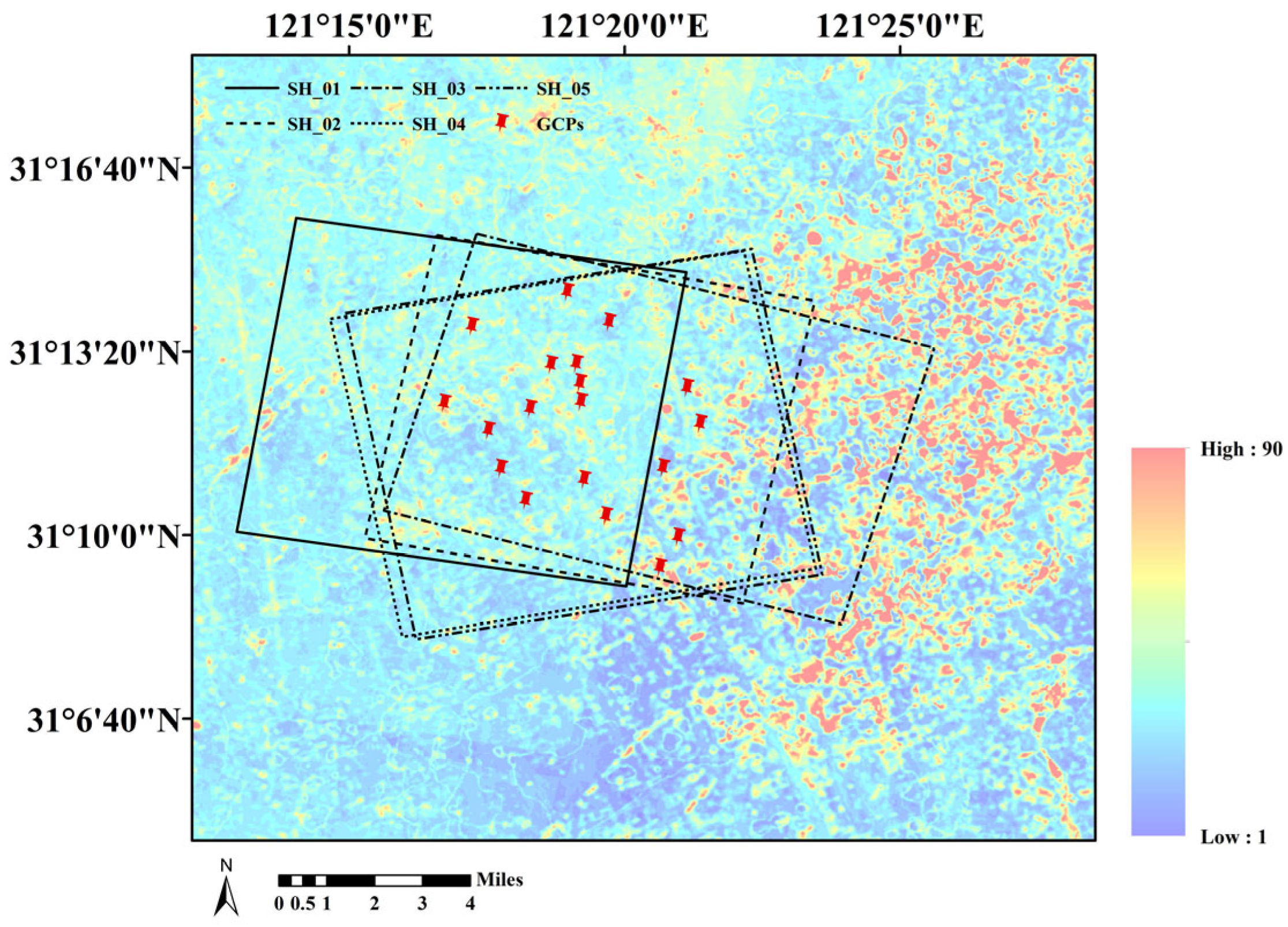
2.1.2. Study Area and Gaofen-3 Image Data

Several Gaofen-3 spotlight mode SAR images were collected in three research areas (Henan, Shaanxi, and Shanghai). The image datasets in the three areas were acquired at different look angles from either ascending or descending orbits.

In the first study area, Henan, the terrain is mainly mountainous, including hills and plains. The average altitude varies significantly in different terrains. The period of these image data was from October 2016 to December 2019. The characteristics of the dataset in this area are as follows: the side-looking direction of the SAR system is right looking; the range of incidence angle is ~21.1–40.6° (

Table 2. Image data information of Henan.

Image ID	Orbit	Look Direction	Incidence Angle (°)	Acquisition Time
HN_01	Descending	Right	33.8	14 October 2016
HN_02	Descending	Right	25.7	7 August 2018
HN_03	Descending	Right	40.4	29 August 2019
HN_04	Descending	Right	37.4	6 December 2019
HN_05	Descending	Right	43.2	11 December 2019
HN_06	Descending	Right	37.4	7 November 2019
HN_07	Ascending	Right	37.6	9 November 2019
HN_08	Ascending	Right	30.2	14 November 2019
HN_09	Ascending	Right	21.1	19 November 2019
HN_10	Descending	Right	40.6	24 November 2019

). The selected SAR images and control-point distributions are shown in Figure 2.

The second study area, Shaanxi, had an elevation of ~330–2645 m. The terrain is high in the north and south and low in the middle. As shown in

Table 3. Image data information of Shaanxi.

Image ID	Orbit	Look Direction	Incidence Angle (°)	Acquisition Time
SX_01	Descending	Right	32.0	14 August 2018
SX_02	Descending	Right	32.0	11 December 2018
SX_03	Ascending	Right	28.3	28 July 2018
SX_04	Ascending	Right	39.5	4 August 2018
SX_05	Ascending	Right	19.1	29 September 2018

, the acquisition time of the image data was concentrated in 2018, and the side-looking direction of the SAR system was right looking. The incidence angle of the images ranged from ~19.1–32.0°. The selected SAR images and control-point distributions are shown in Figure 3.

The elevation of the third study area, Shanghai, is high in the southeast and low in the northwest, with a ground elevation of ~3.5–4.5 m and an average elevation of 3.87 m. Data were collected between March and April 2018. The characteristics of the dataset are shown in

Table 4. Image data information of Shanghai.

Image ID	Orbit	Look Direction	Incidence Angle (°)	Acquisition Time
SH_01	Descending	Right	42.7	9 March 2018
SH_02	Descending	Right	23.6	9 April 2018
SH_03	Descending	Left	35.0	27 March 2018
SH_04	Ascending	Right	28.9	23 March 2018
SH_05	Ascending	Right	33.0	4 April 2018

, where only one image has the incidence angle direction to the left, and the other images have the incidence angle direction to the right; the range of incidence angle is ~23.6–42.7°. The selected SAR images and control-point distributions are shown in Figure 4.

2.2. Methods

Since all targets with different altitude coordinates are projected onto a single SAR image, a single SAR image can only locate the two-dimensional coordinates of the target point and cannot provide the altitude information of the target point [18,19]. However, two SAR images with a certain intersection angle can form a stereo-image pair to locate the three-dimensional coordinates of the target point [20]. Three-dimensional coordinate positioning uses the coordinates ${(\mathrm{x}}_1{, \mathrm{y}}_1)$ and $\left({\mathrm{x}}_2{, \mathrm{y}}_2\right)$ of the image points with the same name on the stereo-image pair, and the range information and Doppler information during radar imaging. Two sets of conditional equations are established according to the range equation and Doppler equation. By solving these two sets of conditional equations, the three-dimensional coordinates of the target points can be obtained [21].

2.2.1. Stereo-Image Pair Acquisition Method

SAR stereo-image pairs exhibit certain image overlaps. According to the relationship between the two flight observation angles, they can be divided into ipsilateral and heterolateral stereo observations [22]. Ipsilateral stereo observation means that the radar captures images from the target area twice from the same side as the target area (Figure 5a). Heterolateral stereo observation implies that the radar captures images from the target area from both sides of the target area (Figure 5b).

2.2.2. 3-D Localization Method for Spaceborne SAR Imagery

Generally, the geometric relationship of a satellite remote sensing image is used as its mathematical model. The system error was eliminated in the adjustment process according to the positioning consistency principle of the same name points, and the corresponding object coordinates were calculated. According to the different geometric geolocation models, the main geolocation methods for spaceborne SAR imagery can be divided into the geolocation method based on the Range and Doppler model (RDM) [23] and the geolocation method based on the RPC model [24]. Yingdan verified through experiments that the 3-D localization method based on the RPC model can achieve the same accuracy as the 3-D localization method based on the strict imaging geometry model [25]. Under the premise of ensuring the same processing accuracy, the RPC model has higher versatility and is more convenient to process. Therefore, this study used the RPC model to perform the 3-D localization of the Gaofen-3 image.

The RPC model associates the image point coordinates $\left(\mathrm{r}, \mathrm{c}\right)$ with the corresponding ground point coordinates $\left(P,L,H\right)$ through the polynomial model. The association of two coordinates can be written as:

$$\left\{\begin{array}{l}r=\frac{Nu{m}_L\left(P,L,H\right)}{De{n}_L\left(P,L,H\right)}\\ c=\frac{Nu{m}_S\left(P,L,H\right)}{De{n}_S\left(P,L,H\right)}\end{array}\right.$$

(1)

where P, L, and H are coordinate values of the latitude, the longitude, and the elevation, respectively; r and c are the row and column index of pixels in the image;$Nu{m}_L\left(P,L,H\right)$, ${Den}_L(P, L, H)$, ${Num}_S(P, L, H)$, and ${Den}_S(P, L, H)$ are the terms of the third-order polynomial of $(P, L, H)$.

By expanding Equation (1) to the first-order term according to Taylor’s formula, Equation (2) is obtained as follows:

$$\left\{\begin{array}{l}r=\widehat{r}+\frac{\partial r}{\partial P}\Delta P+\frac{\partial r}{\partial L}\Delta L+\frac{\partial r}{\partial H}\Delta H\\ c=\widehat{c}+\frac{\partial c}{\partial P}\Delta P+\frac{\partial c}{\partial L}\Delta L+\frac{\partial c}{\partial H}\Delta H\end{array}\right.$$

(2)

where $\widehat{r}$ and $\widehat{c}$ are the initial values of row and column coordinates, respectively; $\frac{\partial r}{\partial P}$, $\frac{\partial r}{\partial L}$, $\frac{\partial r}{\partial H}$, $\frac{\partial c}{\partial P}$, $\frac{\partial c}{\partial L}$, and $\frac{\partial c}{\partial H}$ are first derivatives; $\Delta P$, $\Delta L$, and $\Delta H$ are corrections of the latitude, the longitude and the elevation, respectively.

Therefore, the error equation of the space front intersection is Equation (3), and the object square space coordinates of the image points can be solved by combining the observation of multiple image points with Equation (3).

$$\left\{\begin{array}{l}{v}_r=\left[\frac{\partial r}{\partial P}\frac{\partial r}{\partial L}\frac{\partial r}{\partial H}\right]\left[\begin{array}{l}\Delta P\\ \Delta L\\ \Delta H\end{array}\right]-\left(r-\widehat{r}\right)\\ v_c=\left[\frac{\partial c}{\partial P}\frac{\partial c}{\partial L}\frac{\partial c}{\partial H}\right]\left[\begin{array}{l}\Delta P\\ \Delta L\\ \Delta H\end{array}\right]-\left(c-\widehat{c}\right)\end{array}\right.$$

(3)

where $v_r$ and $v_c$ are correction value of pixel coordinates.

From the above equations, we can see that for an unknown ground point, there are three unknowns in the forward solution method and that the two identical image points of the ground point in the stereo-image pair can obtain four equations. Therefore, the least-squares method can be used to obtain the square coordinates of the ground point. The specific steps were as follows:

• The initial iteration value ${(P}_0{, L}_0{, H}_0)$ of the unknown ground point was set. In general, the average elevation of the corresponding region of the stereo-image pair can be used as the initial value.
• Using the initial ground coordinates and observed values of the image point coordinates of the same name, the coefficients in the error equation were solved according to Equation (3).
• The least-squares method was used to obtain the correction value of the ground unknown point coordinates.
• When the correction values $(\Delta P, \Delta L, \Delta H)$ exceed the allowable limit value, the correction value calculated in the third step was superimposed on ${(P}_0{, L}_0{, H}_0)$. In this way, we can get the new initial coordinates of the unknown points on the ground, and then start the calculation from the second step down.
• When the correction value $(\Delta P, \Delta L, \Delta H)$ is within the limit value, the loop breaks, representing the end of the calculation. In this case, ${(P}_0{ + \Delta P, L}_0{ + \Delta L, H}_0 + \Delta H)$ is the true value of an unknown point on the ground.

2.2.3. Optimizing the RPC Model

Owing to the errors in the observation parameters of the range-Doppler model, the RPC model obtained by fitting has errors. The analysis shows that the system time-delay error in the range direction and atmospheric delay error can be eliminated using the geometric calibration method. The specific geometric calibration method is described in detail in a previous study [26].

2.2.4. Evaluation of 3-D Stereo Accuracy

Using the image point coordinates of the same name points on the stereo-image pair (the same name points are the GCPs of the stereo-images overlap), the 3-D coordinates of the same name points can be calculated through the forward intersection and the RPC model. By comparing the 3-D coordinates calculated from all SAR images and field measurements, the RMSE can be obtained to evaluate 3-D localization accuracy [27].

For the standard 3-D coordinates, the Universal Transverse Mercator (UTM) coordinate system was used for the plane, and the ground height in the World Geodetic System 1984 (WGS84) coordinate system was used for the elevation. 3-D localization accuracy is generally evaluated in two dimensions: plane and elevation. The plane accuracy of 3-D localization is reflected by the RMSE of the north, east, and plane (north and east directions combined), and the elevation accuracy is reflected by the RMSE of the height. The specific technical process of stereotaxic accuracy evaluation is as follows is expressed as follows:

• Pick the SAR spotlight image; the coordinates ${(\mathrm{x}}_1{, \mathrm{y}}_1)$ and ${(\mathrm{x}}_2{, \mathrm{y}}_2)$ of the GCP in the stereo-image pair were obtained.
• The 3-D coordinates of the point with the same name ${(\mathrm{X}}_1{, \mathrm{Y}}_1{, \mathrm{Z}}_1)$ were obtained using the RPC model, and the coordinates were compared with the coordinates of the target point. The field measurement coordinates $(\mathrm{X}, \mathrm{Y}, \mathrm{Z})$ were transformed into plane coordinates and the elevation in the UTM coordinate system.
• In the UTM coordinate system, the RMSE of the north direction, east direction, plane, and elevation height of all checkpoints of the stereo-image pair was calculated.

3. Results and Discussion

The 3-D localization accuracy was evaluated for the three study areas, and the results are summarized in

Table 5. Estimation of 3-D localization accuracy in Zhengzhou, Henan Province.

Stereopairs Acquisition Method	Stereopair ID	Image ID	Time Width & Bandwidth (μs & MHz)	GCPs	Intersection Angle (°)	Before/After Model Optimization	RMSE (m)
							East	North	Plane	Height
Heterolateral	HN_A	HN_01	240 & 45.000	6	83.7	Before	7.022	1.978	7.295	37.026
		HN_07	240 & 54.990			After	5.208	1.440	5.403	0.580
	HN_B	HN_01	240 & 45.000	5	75.4	Before	3.887	1.396	4.130	33.374
		HN_08	240 & 45.000			After	4.383	1.075	4.513	0.803
	HN_C	HN_01	240 & 45.000	6	65.7	Before	2.338	1.215	2.635	30.538
		HN_09	240 & 45.000			After	4.945	0.820	5.012	1.288
	HN_D	HN_02	240 & 45.000	5	74.5	Before	9.168	0.812	9.203	33.546
		HN_07	240 & 54.990			After	5.221	0.826	5.286	0.115
	HN_E	HN_02	240 & 45.000	4	66.5	Before	5.983	0.529	6.007	30.792
		HN_08	240 & 45.000			After	4.409	0.512	4.439	1.234
	HN_F	HN_02	240 & 45.000	5	57.1	Before	4.569	0.136	4.571	28.604
		HN_09	240 & 45.000			After	4.985	0.220	4.990	1.682
	HN_G	HN_03	240 & 54.990	6	88.7	Before	1.482	1.800	2.332	42.635
		HN_07	240 & 54.990			After	2.047	1.306	2.428	3.575
	HN_H	HN_03	240 & 54.990	5	82.9	Before	1.933	1.337	2.351	37.687
		HN_08	240 & 45.000			After	0.907	1.133	1.452	1.634
	HN_I	HN_03	240 & 54.990	6	73.7	Before	3.973	0.953	4.086	33.516
		HN_09	240 & 45.000			After	0.930	0.680	1.152	0.545
	HN_J	HN_04	240 & 45.000	7	87.7	Before	4.824	1.039	4.935	38.371
		HN_07	240 & 54.990			After	4.686	1.036	4.799	0.558
	HN_K	HN_04	240 & 45.000	4	79.4	Before	1.561	0.539	1.652	34.352
		HN_08	240 & 45.000			After	3.816	0.745	3.888	0.868
	HN_L	HN_04	240 & 45.000	6	69.5	Before	0.448	0.154	0.474	30.911
		HN_09	240 & 45.000			After	4.140	0.338	4.154	1.512
	HN_M	HN_05	240 & 54.990	5	85.3	Before	0.222	0.757	0.789	43.717
		HN_07	240 & 54.990			After	2.131	0.863	2.300	3.253
	HN_N	HN_05	240 & 54.990	3	86.2	Before	3.592	0.300	3.605	38.178
		HN_08	240 & 45.000			After	1.083	0.294	1.123	1.074
	HN_O	HN_05	240 & 54.990	5	76.2	Before	5.927	0.613	5.958	33.604
		HN_09	240 & 45.000			After	1.037	0.490	1.147	0.204
	HN_P	HN_06	240 & 45.000	6	87.7	Before	5.907	1.954	6.222	37.892
		HN_07	240 & 54.990			After	5.376	1.712	5.642	0.343
	HN_Q	HN_06	240 & 45.000	4	79.4	Before	2.980	1.672	3.417	33.961
		HN_08	240 & 45.000			After	4.745	1.628	5.016	1.111
	HN_R	HN_06	240 & 45.000	5	69.5	Before	1.308	1.221	1.789	30.773
		HN_09	240 & 45.000			After	5.174	1.088	5.288	1.575
	HN_S	HN_07	240 & 54.990	6	88.6	Before	0.444	0.422	0.612	43.642
		HN_10	240 & 54.990			After	0.488	0.479	0.684	4.540
	HN_T	HN_08	240 & 45.000	5	82.4	Before	4.165	0.339	4.179	38.494
		HN_10	240 & 54.990			After	0.878	0.569	1.046	2.395
	HN_U	HN_09	240 & 45.000	5	73.6	Before	6.649	0.631	6.679	34.067
		HN_10	240 & 54.990			After	1.232	0.555	1.351	1.048
Ipsilateral	HN_V	HN_02	240 & 45.000	5	21.2	Before	26.648	6.579	27.448	13.320
		HN_05	240 & 54.990			After	7.562	3.329	8.262	7.169

,

Table 6. Estimation of 3-D localization accuracy in Weinan, Shaanxi Province.

Stereopairs Acquisition Method	Stereopair ID	Image ID	Time Width & Bandwidth (μs & MHz)	GCPs	Intersection Angle (°)	Before/After Model Optimization	RMSE (m)
							East	North	Plane	Height
Heterolateral	SX_A	SX_01	240 & 45.000	6	71.4	Before	17.342	12.085	21.137	33.004
		SX_03	240 & 35.009			After	4.560	1.691	4.863	0.384
	SX_B	SX_01	240 & 45.000	5	83.7	Before	18.292	11.190	21.443	36.506
		SX_04	240 & 45.000			After	6.239	1.677	6.460	1.562
	SX_C	SX_01	240 & 45.000	6	61.6	Before	12.221	13.629	18.305	26.083
		SX_05	240 & 35.009			After	2.130	2.647	3.397	5.923
	SX_D	SX_02	240 & 45.000	5	71.4	Before	5.302	2.493	5.859	33.457
		SX_03	240 & 35.009			After	5.838	2.715	6.439	0.567
	SX_E	SX_02	240 & 45.000	4	83.6	Before	9.794	1.827	9.963	37.870
		SX_04	240 & 45.000			After	6.975	1.925	7.236	1.600
	SX_F	SX_02	240 & 45.000	5	61.6	Before	3.367	4.102	5.307	25.322
		SX_05	240 & 35.009			After	0.652	3.880	3.934	5.540

and

Table 7. Estimation of 3-D localization accuracy in Pudong, Shanghai.

Stereopairs Acquisition Method	Stereopair ID	Image ID	Time Width & Bandwidth (μs & MHz)	GCPs	Intersection Angle (°)	Before/After Model Optimization	RMSE (m)
							East	North	Plane	Height
Heterolateral	SH_A	SH_02	240 & 35.009	6	66.6	Before	7.808	2.138	8.096	31.309
		SH_03	240 & 45.000			After	4.130	2.414	4.783	1.656
	SH_B	SH_02	240 & 35.009	8	63.0	Before	11.178	1.118	11.234	29.434
		SH_04	240 & 35.009			After	9.511	1.213	9.588	2.242
	SH_C	SH_02	240 & 35.009	8	67.4	Before	11.295	1.209	11.359	27.889
		SH_05	240 & 45.000			After	8.057	1.461	8.188	4.893

and Figure 6. Table 5, Table 6 and Table 7 show the specific information of the stereo-image pairs in the three study areas and the 3-D localization accuracy before and after RPC model optimization. The line chart in Figure 6 reflects the variation in the 3-D localization accuracy after operation in ascending order of intersection angle size.

Through all the test data and charts, some test conclusions of the Gaofen-3 spotlight stereo image for 3-D localization can be drawn.

For the RPC model before optimization:

• Overall, the elevation accuracy was poor, at ±33.546 m (the median elevation accuracy of all stereo-image pairs), which is worse than 37 m in most cases. The plane accuracy was better at ±5.307 m (the median plane accuracy of all stereo-image pairs), which is better than 10 m in general.
• The plane accuracy of the 3-D localization of the ipsilateral stereo-image pair was lower than that of the heterolateral stereo-image pair, and the planar accuracy of the ipsilateral stereo-image pair HN_V was the worst at 27.448 m. The plane accuracy of the heterolateral stereo-image for SX_B was the worst at 21.443 m.
• As shown in Figure 6, the 3-D localization accuracy of all the stereo-image pairs fluctuated significantly. In general, the larger the stereo intersection angle, the worse the elevation accuracy. The plane accuracy was less affected by the stereo intersection angle.

For the geometrically calibrated RPC model:

• After geometric calibration, the accuracy of 3-D localization was greatly improved. The elevation accuracy was ±1.512 m (the median elevation accuracy of all optimized stereo-image pairs), which was mostly better than 5 m. The plane accuracy was ±4.783 m (the median plan accuracy of all optimized stereo-image pairs), which is better than 6 m in general. The elevation accuracy was improved by approximately 30 m, and the improvement effect was good for the stereo image, with a plane accuracy better than 5 m, and the improvement effect was approximately 10 m. For stereo images whose plane accuracy is worse than 5 m before optimization, the plane accuracy is generally improved.
• The observed ipsilateral stereo-image pair HN_V was significantly better than the other stereo-image pairs in the improvement of plane accuracy, and the difference in plane accuracy before and after optimization was 19.186 m. The improvement in elevation accuracy was the worst, and the elevation difference before and after optimization was 6.151 m.
• As shown in Figure 6, the fluctuation range of the 3-D localization accuracy became smaller and more stable within a certain range. The stereo accuracy after geometric calibration was less affected by the intersection angle.

Theoretically, heterolateral stereo images have noticeable disparities and large base-to-height ratios, and the accuracy of heterolateral 3-D localization is higher than that of ipsilateral 3-D localization, which was also confirmed by our experiment. The initialized RPC model was affected by the sensors, platform ephemeral, terrain height, and processor. Before model optimization, the elevation accuracy of 3-D localization was relatively low. The error of the stereo calibration was mainly in the range direction, while the stereo geometry calibration mainly improved this error; therefore, the optimization effect on the elevation accuracy was more noticeable. Most of the incidence angles of the selected heterolateral stereo-image pairs were similar, which approximates symmetric 3-D localization. Localization of the ipsilateral stereo-image pair was asymmetric. Therefore, the improvement of the plane accuracy of heterolateral 3-D localization had a small impact; however, it had a large impact on the improvement of the plane accuracy of ipsilateral 3-D localization. Geometric calibration technology has little influence on improving the plane accuracy of 3-D localization; however, it has a great impact on the improvement of the accuracy of the ipsilateral 3-D localization plane.

4. Conclusions

This study evaluated the accuracy of the 3-D localization of Gaofen-3 spotlight images. In the case of no control points based on the RPC model, the 3-D localization of the Gaofen-3 spotlight image yielded poor elevation accuracy and unstable plane accuracy. The RPC model was optimized using geometric calibration technology to improve the accuracy of the 3-D localization. Geometric calibration improves the range error of the slant range image, greatly improves the elevation accuracy, and stabilizes plane accuracy. In the case of no ground control points (GCPs), based on the RPC model, the plane accuracy was better than 10 m in general, and the elevation accuracy was worse than 37 m in general. After the RPC model was optimized using geometric calibration technology, the elevation accuracy was significantly improved, which was generally better than 5 m. The plane accuracy was also improved, and it was generally better than 6 m. In addition, the effect of the optimization of geometric calibration on the plane accuracy is affected by the anterolateral stereo-image pairs, and the improvement in the plane accuracy of the ipsilateral stereo-image pairs was more noticeable than that of the symmetric stereo-image pair. However, owing to the lack of test data for the asymmetric stereo-image pair, this conclusion requires further study.

References

- Zhang, Q.; Yan, S.; Lü, M.; Zhang, L.; Liu, G. Accurate extraction and analysis of mountain glacier surface motion with GF-3 imagery. J. Glaciol. Geocryol. 2021, 43, 1594–1605. [Google Scholar]
- Zhang, L.; Wang, Z.; Ye, K.; Chang, D. Coastline Extraction Method Based on Multi Feature Classification of Full Polarization SAR Image. Remote Sens. Inf. 2022, 37, 58–65. [Google Scholar]
- Lin, X.; Luo, D.; Lian, R.; Wei, W. Application of GF-3 Spotlight Mode Data in Urban Flood Disaster Emergency Response. Geospat. Inf. 2021, 20, 1–4. [Google Scholar]
- Zhang, Q. System Design and Key Technologies of the GAOFEN-3 Satellite. Acta Geod. Cartogr. Sin. 2017, 46, 269–277. [Google Scholar]
- Gao, L. Basic Method and Practice of SAR Photogrammetric Processing; PLA Information Engineering University: Zhengzhou, China, 2004. [Google Scholar]
- Toutin, T.; Chenier, R. 3-D Radargrammetric Modeling of RADARSAT-2 Ultrafine Mode: Preliminary Results of the Geometric Calibration. IEEE Geosci. Remote Sens. Lett. 2009, 6, 282–286. [Google Scholar] [CrossRef]
- Toutin, T.; Blondel, E.; Clavet, D.; Schmitt, C. Stereo radargrammetry with Radarsat-2 in the Canadian Arctic. IEEE Trans. Geosci. Remote Sens. 2013, 51, 2601–2609. [Google Scholar] [CrossRef]
- Toutin, T. Impact of Radarsat-2 SAR Ultrafine-Mode Parameters on Stereo-Radargrammetric DEMs. IEEE Trans. Geosci. Rem. Sens. 2010, 48, 3816–3823. [Google Scholar] [CrossRef]
- Papasodoro, C.; Royer, A.; Langlois, A.; Berthier, E. Potential of RADARSAT-2 stereo radargrammetry for the generation of glacier DEMs. J. Glaciol. 2016, 62, 486–496. [Google Scholar] [CrossRef]
- Capaldo, P.; Crespi, M.; Fratarcangeli, F.; Nascetti, A.; Pieralice, F. High-Resolution SAR Radargrammetry: A First Application With COSMO-SkyMed SpotLight Imagery. IEEE Trans. Geosci. Rem Sens. 2011, 8, 1100–1104. [Google Scholar] [CrossRef]
- Agrawal, R.; Das, A.; Rajawat, A. Accuracy Assessment of Digital Elevation Model Generated by SAR Stereoscopic Technique Using COSMO-Skymed Data. J. Indian Soc. Remote Sens. 2018, 46, 1739–1747. [Google Scholar] [CrossRef]
- Eldhuset, K.; Weydahl, D.J. Geolocation and stereo height estimation using TerraSAR-X spotlight image data. IEEE Trans. Geosci. Remote Sens. 2011, 49, 3574–3581. [Google Scholar] [CrossRef]
- Zhang, G.; Li, Z.; Pan, H.; Qiang, Q.; Zhai, L. Orientation of Spaceborne SAR Stereo Pairs Employing the RPC Adjustment Model. IEEE Trans. Geosci. Remote Sens. 2011, 49, 2782–2792. [Google Scholar] [CrossRef]
- Zhang, G.; Li, Z. RPC-based adjustment model for TerraSAR-X stereo orientation. Sci. Surv. Mapp. 2011, 36, 146–148. [Google Scholar]
- Balss, U.; Eineder, M.; Fritz, T.; Breit, H.; Minet, C. Techniques for High Accuracy Relative and Absolute Localization of TerraSAR-X/TanDEM-X Data. In Proceedings of the 2011 IEEE International Geoscience and Remote Sensing Symposium, Vancouver, BC, Canada, 24–29 July 2011. [Google Scholar]
- Balss, U.; Gisinger, C.; Cong, X.; Brcic, R.; Hackel, S.; Eineder, M. Precise Measurements on the Absolute Localization Accuracy of TerraSAR-X on the Base of Far-Distributed Test Sites. In Proceedings of the 10th European Conference on Synthetic Aperture Radar (EUSAR), Berlin, Germany, 5 June 2014. [Google Scholar]
- Balss, U.; Gisinger, C.; Eineder, M. Measurements on the Absolute 2-D and 3-D Localization Accuracy of TerraSAR-X. Remote Sens. 2018, 10, 656. [Google Scholar] [CrossRef]
- Cumming, I.G.; Wong, F.H. Digital Processing of Synthetic Aperture Radar Data: Algorithms and Implementation; Artech House: Boston, MA, USA, 2005. [Google Scholar]
- Liu, Y.; Xing, M.; Sun, G.; Lv, X.; Bao, Z.; Hong, W.; Wu, Y. Echo model analyses and imaging algorithm for high-resolution SAR on high-speed platform. IEEE Trans. Geosci. Remote Sens. 2012, 50, 933–950. [Google Scholar] [CrossRef]
- Li, D.; Liu, J.Y. A stereo positioning method of GaoFen-3 SAR images under different time and space conditions. J. Univ. Chin. Acad. Sci. 2021, 38, 519–523. [Google Scholar]
- Benyi, C.; Yong, F. The principles of positioning with space-borne SAR images. In Proceedings of the IEEE International Geoscience and Remote Sensing Symposium, Toronto, ON, Canada, 24–28 June 2002; Volume 4, pp. 1950–1952. [Google Scholar] [CrossRef]
- Chen, P.H.; Dowman, I.J. Space intersection from ERS-1 synthetic aperture radar images. Photogramm. Rec. 1996, 15, 561–573. [Google Scholar] [CrossRef]
- Sansosti, E.; Berardino, P.; Manunta, M.; Serafino, F.; Fornaro, G. Geometrical SAR image registration. IEEE Trans. Geosci. Remote Sens. 2006, 44, 2861–2870. [Google Scholar] [CrossRef]
- Zhang, G.; Fei, W.; Li, Z.; Zhu, X.; Tang, X. Analysis and Test of the Substitutability of the RPC Model for the Rigorous Sensor Model of Spaceborne SAR Imagery. Acta Geod. Cartogr. Sin. 2010, 39, 264. [Google Scholar]
- Wu, Y. Accurate Geometric Positioning of Spaceborne SAR Remote Sensing Imagery; Wuhan University: Wuhan, China, 2010. [Google Scholar]
- Deng, M.; Zhang, G.; Cai, C.; Xu, K.; Zhao, R.; Guo, F.; Suo, J. Improvement and Assessment of the Absolute Positioning Accuracy of Chinese High-Resolution SAR Satellites. Remote Sens. 2019, 11, 1465. [Google Scholar] [CrossRef]
- Raggam, H.; Gutjahr, K.; Perko, R.; Schardt, M. Assessment of the Stereo-Radargrammetric Mapping Potential of TerraSAR-X Multibeam Spotlight Data. IEEE Trans. Geosci. Remote Sens. 2010, 48, 971–977. [Google Scholar] [CrossRef]