Article

Multimodal Deep Learning for Rice Yield Prediction Using UAV-Based Multispectral Imagery and Weather Data

1
The United Graduate School of Agricultural Science, Gifu University, Gifu 5011193, Japan
2
Faculty of Agricultural Engineering and Technology, Sylhet Agricultural University, Sylhet 3100, Bangladesh
3
Graduate School of Natural Science and Technology, Gifu University, Gifu 5011193, Japan
4
Faculty of Agriculture and Marine Science, Kochi University, Kochi 7838502, Japan
5
Graduate School of Agricultural Science, Tohoku University, Miyagi 9808572, Japan
6
Faculty of Food and Agricultural Sciences, Fukushima University, Fukushima 9601296, Japan
7
Faculty of Biological Sciences, Gifu University, Gifu 5011193, Japan
8
Artificial Intelligence Advanced Research Center, Gifu University, Gifu 5011193, Japan
*
Author to whom correspondence should be addressed.
Current address: Faculty of Applied Biological Sciences, Gifu University, Yanagido, Gifu 5011193, Japan.
Remote Sens. 2023, 15(10), 2511; https://doi.org/10.3390/rs15102511
Submission received: 6 April 2023 / Revised: 2 May 2023 / Accepted: 9 May 2023 / Published: 10 May 2023

Abstract

:
Precise yield predictions are useful for implementing precision agriculture technologies and making better decisions in crop management. Convolutional neural networks (CNNs) have recently been used to predict crop yields in unmanned aerial vehicle (UAV)-based remote sensing studies, but weather data have not been considered in modeling. The aim of this study was to explore the potential of multimodal deep learning on rice yield prediction accuracy using UAV multispectral images at the heading stage, along with weather data. The effects of the CNN architectures, layer depths, and weather data integration methods on the prediction accuracy were evaluated. Overall, the multimodal deep learning model integrating UAV-based multispectral imagery and weather data had the potential to develop more precise rice yield predictions. The best models were those trained with weekly weather data. A simple CNN feature extractor for UAV-based multispectral image input data might be sufficient to predict crop yields accurately. However, the spatial patterns of the predicted yield maps differed from model to model, although the prediction accuracy was almost the same. The results indicated that not only the prediction accuracies, but also the robustness of within-field yield predictions, should be assessed in further studies.

Graphical Abstract

1. Introduction

Precision agriculture is expected to contribute to the enhancement of crop productivity by collecting, processing, and analyzing temporal and spatial data and combining them with other information to support management decisions based on the efficient use of resources. Yield predictions are crucial sources of information in site-specific agriculture, allowing farmers to make informed decisions about resource allocation and management practices based on a detailed understanding of the spatial and temporal variabilities in crop performance [1]. Farmers can improve crop production and implement optimal farm management techniques by carefully monitoring biophysical quantities, particularly biomass and grain yield [2]. In the agricultural sector, timely, nondestructive, inexpensive, and reliable large-scale yield forecasts are important and prerequisite for preventing climate risks and ensuring food security [3]. Thus, yield monitoring and satellite-based remote sensing technologies have been developed to quantify the spatial distribution of crop yields in large-scale farming practices. Moreover, the precision agriculture demand for low-cost and accurate crop yield and quality prediction tools is urgently growing, especially in Asian countries, where smallholders are dominant [4].
Traditional crop yield measurement approaches are destructive and laborious [5]. Yield estimation models such as WOFOST (WOrld FOod STudies), APSIM (Agricultural Production Systems sIMmulator), and DSSAT (Decision Support System for Agro-Technology Transfer Model) can simulate crop development, crop growth, and yield formulation at a daily time step [6]. However, such models are very dependent on substantial and specific input information on the local soils, crop management practices, and weather data [3], and require massive computational costs [7]. Since process-based models for simulating physiological mechanisms are constrained by the availability of data for parameterization, data analytical approaches using statistical and machine learning models are recommended as possible alternatives.
Due to advancements in environments storing big data and high-performance computational technologies, machine learning approaches have become a popular technique for modeling intercorrelated and nonlinear relationships [8]. Recently, artificial intelligence and other machine learning algorithms have gradually replaced traditional statistical models (e.g., linear regression models) due to the flexibility of self-adaptive learning methods from large samples [5]. With minimal or no human intervention, machine learning algorithms can develop innovative methods to solve real-world problems and assist farmers in decision-making [9].
Since the 1970s, satellite data have been extensively employed to predict crop yields [2]. To establish a precise satellite-based yield prediction model for a variety of crops, the potential of machine learning approaches, such as artificial neural networks (ANN) [10,11], random forest regression (RF) [12,13,14,15], and support vector regression (SVR) [16,17], has been examined. However, the limited spatial and temporal resolution of satellite data hinders precise yield predictions [18]. Therefore, unmanned aerial vehicles (UAVs) have been widely used to collect data due to their superior spatial, spectral, and temporal resolutions compared to airborne and satellite platforms [19].
Vegetation indices (VIs) from multispectral and RGB (red, green, and blue) images are a conventional proxy for crop monitoring [20]. The physiological and geometric properties of vegetation, such as the leaf chlorophyll content, leaf area index (LAI), nitrogen concentration, plant height, biomass yield and grain yield, can be estimated from canopy spectral information derived from UAV-based multispectral and hyperspectral imagery [19]. However, Zhou et al. [4] reported that machine learning methods based on vegetation index values derived from UAV-based remote sensing data, such as the RF, SVR, and ANN methods, did not outperform linear regression in terms of their wheat yield prediction accuracies. The linear regression model may be able to provide approximate crop yield predictions based on reflectance or vegetation indices. Due to the higher spatial resolution of UAV-based remote sensing data, compared to satellite-based remote sensing data, a region of interest of raw UAV images consists of a multidimensional matrix, which is difficult to directly treat as input data for machine learning. Therefore, in the preprocessing steps of general machine learning approaches, the pixel values of images within a certain region of interest are aggregated into statistics such as the mean and median values. However, this process causes spatial features that may be important for yield prediction to be lost. To overcome the drawbacks of general data preprocessing for UAV-based remote sensing and machine learning approaches, a convolutional neural network (CNN) was used to precisely predict wheat [21,22] with the lowest RMSE (0.94 t ha−1) [22] and rice grain yields [5,23], with a coefficient of determination (R2) of 0.499 [23]. The CNN can learn pertinent information from images at different levels, similar to a human brain. The CNN can then extract spatial features of the input images through convolutional, pooling, and fully connected layers. CNNs have frequently been used in a variety of fields for image classification, detection, segmentation, and retrieval problems [24], including image and semantic recognition [25], natural language processing [26], and video analysis tasks [27].
Weather is one of the major environmental factors affecting crop growth and yield. For example, rice yields are largely affected by solar radiation in each growth stage [28]. Furthermore, rice is highly susceptible to heat stress during the flowering stage, and heat stress negatively affects the crop yield [29]. Song et al. [30] assessed the impacts of heat stress on wheat yields using both statistical models and satellite solar-induced chlorophyll fluorescence (SIF) data. An ANN was used to predict winter wheat yield using satellite-based remotely sensed and climate data [31]. Kim et al. [32] developed a deep neural model for predicting crop yields by using satellite imagery and meteorological datasets. To develop a precise yield prediction model on a regional scale, researchers have frequently used satellite-based remote sensing and weather data to establish multimodal deep learning models. To the best of our knowledge, multimodal deep learning methods, that is, the integration of weather data into a CNN model, have rarely been attempted in studies involving UAV-based remote sensing.
CNN models are known for their computational complexity and high memory requirements, which can limit their applicability in resource-constrained environments. Several factors can impact the efficiency of CNN models, including the network architecture, training algorithms, optimization techniques, and available hardware. Using relatively small network architectures and reducing the number of parameters can help lower the computational costs of training and prediction for practical applications. However, it is well known that deepening and widening CNN architectures can enhance the model performance [33]. Therefore, there is a balance between the model performance and computational cost when designing CNN architectures.
The objective of this study was to develop a multimodal deep learning model to predict rice grain yield using UAV images at the heading stage and weather data. The effects of CNN layers, layer depths, and weather data types on model performance were assessed in terms of prediction accuracy and feasibility in terms of computational time. Furthermore, the predicted yield maps were compared using the best-fitted model to evaluate the robustness of the model predictions. Although CNN models can extract important features related to crop yield at a time when image data is captured, other environmental external factors hereafter would affect final crop yield. Thus, incorporating weather data after image acquisitions into CNN models is hypothesized to enhance the precision of the yield prediction model. Increasing the depth of the architecture after the integration of weather and image data may also contribute to improving yield prediction accuracy because it can learn complex relationships between temporal and visual data. To establish a practical yield prediction model, a wide variety of yield and image data were needed. These yield data were collected from farmers’ fields across Japan over six years.

2. Materials and Methods

2.1. Description of the Study Site

The research sites were located in Miyagi (140°58′E, 38°23′N), Gifu (136°36′E, 35°16′N and 137°06′E, 35°38′N), and Kochi (133°39′E, 33°36′N) Prefectures in Japan, all of which are located in the East Asian monsoon climate zone (Table 1). This region is known for its abundant year-round rainfall [34] and is ideal for cultivating rice. Kochi Prefecture, located in the southern part of Japan, has higher average temperatures and precipitation levels than the central region (Gifu Prefecture) and the northern region (Miyagi Prefecture) [34]. The primary soil type in all regions is gray lowland soil, except for one area in Gifu Prefecture (137°06′E, 35°38′N) where the major soil type is brown forest soil [35].

2.2. Field Experimentation, Sampling Procedures and Data Collection

Rice yield surveys were conducted in 22 farmers’ fields in Japan over six years (2017–2022) (Table 1). Three of the fields were directly seeded, while the others were transplanted. Nine rice varieties were planted during the growing season from April to May. Crop management was conducted according to local conventional methods. However, strip trials for basal fertilizer application were performed for several fields (Field ID: 14–19) to obtain high yield variations and to determine whether the effect of fertilizer application rates on rice yields could be evaluated using a predicted yield map. In strip trials, long strips are laid out side-by-side in a field, and each strip receives different rates of fertilizer application based on the working width of rice transplanter (approx. 1.9 m). Strip trials are an experimental design widely used for on-farm experimentation. These on-farm experimental fields received different basal fertilizer rates (i.e., 0–500 kg ha−1; N:P:K = 25:6:6 or 24:9:9 depending on the field).
In the maturity stage, the plant samples were harvested with a sickle from an approximately 1.0 m2 area and kept in a warehouse for drying. After drying, the weight of the collected plant samples was measured, and the number of tillers was counted. Then, the samples were threshed and cleaned, and the weight of the threshed grain was measured. A subsample of straw was collected and oven-dried at 70 °C to calculate the moisture content of the aboveground dry matter. To calculate the moisture content of the grain, the samples were oven-dried at 105 °C, and the dry weight was calculated. Finally, the weight of the grain samples was converted to a 15% moisture content. A total of 894 samples were collected throughout all yield surveys. The number of samples obtained in each year was 155, 156, 126, 136, 68, and 253 in 2017, 2018, 2019, 2020, 2021, and 2022, respectively.
Daily meteorological information was collected from the Agro-Meteorological Grid Square Data, NARO (https://amu.rd.naro.go.jp/, accessed on 25 November 2022), for each region. The weather data included precipitation, global solar radiation, temperature (average, minimum, and maximum), average relative humidity, average wind speed, and vapor pressure data [36]. Rice plants gradually complete the transition from the vegetative to reproductive growth stage during the booting and heading stages, and during the mid to late growth stage, the spike color eventually turns yellow, causing the overall spectral pattern of rice to deviate from that of normal green vegetation [24]. The heading stage is suitable for estimating the rice grain yield [37], as it is the vital stage when maximum greenness appears. However, remotely sensed data at the heading stage cannot provide subsequent information. Thus, it is assumed that integrating weather data collected after the heading stage may contribute to improving the yield prediction accuracy. Weather data collected for four weeks after the heading stage were aggregated into either weekly cumulative or monthly cumulative values. The spatial resolution of the provided weather data was 1 km × 1 km; thus, geographically adjacent fields had identical weather data values. The summarized weather data for each unique environment is shown in Table S1.

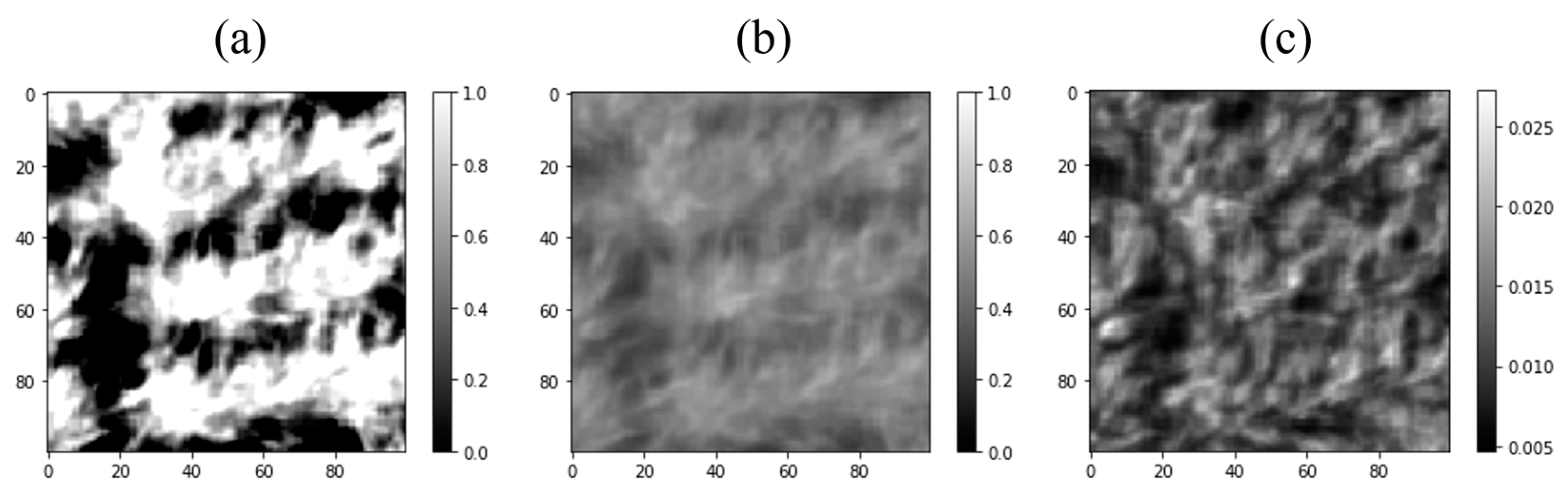
2.3. Image Acquisition and Processing

Multispectral cameras (Sequoia+, Parrot, Paris, France; Rededge Altum, MicaSense, Seattle, USA; and P4 Multispectral, DJI Innovations, Shenzhen, China) mounted on unmanned aerial vehicles (UAVs) were used to obtain multispectral images of rice at the heading stages in each field. The description of three multispectral cameras is shown in Table 2. The prediction model may be influenced by various factors such as different spectral bands, FOV, and spatial resolution. In a preliminary experiment, relationships among spectral reflectance were compared between multispectral cameras by taking images in the same field on the same date. Red-edge band was very sensitive to camera selection; thus, only three bands (green, red, and near-infrared (NIR)) were used for further analysis. The sample images captured through UAV and multispectral cameras are shown in Figure 1. The coordinates of the ground control points (GCPs) for the Sequoia+ camera were determined using global navigation satellite system (GNSS) receivers (M8T, U-Blox, Switzerland) and an open-source program package for GNSS positioning (RTKLIB version 2.4.3) with a 0.01 m precision. The coordinates of the captured images taken by the Rededge-Altum multispectral camera were measured using KlauPPK (Klau Geomatics, Nowra, New South Wales, Australia) with a precision of 0.03 m, allowing for very accurate orthomosaic processing without GCP installation. The coordinates of multispectral images taken by the P4 multispectral camera were calibrated with GCPs by referring to the aerial orthomosaic map products (https://mapps.gsi.go.jp/maplibSearch.do#1, accessed on 10 October 2022). All UAV flights were carried out on sunny days, between 8:00 am and 3:00 pm, under full sunlight and low wind speeds, to avoid image distortion caused by meteorological circumstances. Flights were carried out at the heading stage and just after harvesting plant materials for yield survey. The UAV flew at a height of 65 m above the ground at a speed of 5 m s−1. The forward overlap was set at 85%, while the side overlap was set at more than 65% to successfully generate the orthomosaic images. Using structure-from-motion software (Pix4D mapper version 4.4.12, Pix4D, Prilly, Switzerland), the captured multispectral images were processed to generate reflectance imagery. The ground sample distances ranged from 0.01 to 0.06 m pixel−1. The harvested area was determined using the remotely sensed images obtained just after harvest, and the images of the approximately 1 m2 harvested area were retrieved using GIS software (QGIS 3.22.4). The retrieved images were resampled to 100 pixels × 100 pixels for the neural network (ANN and CNN) inputs using the nearest-neighbor approach.

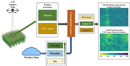
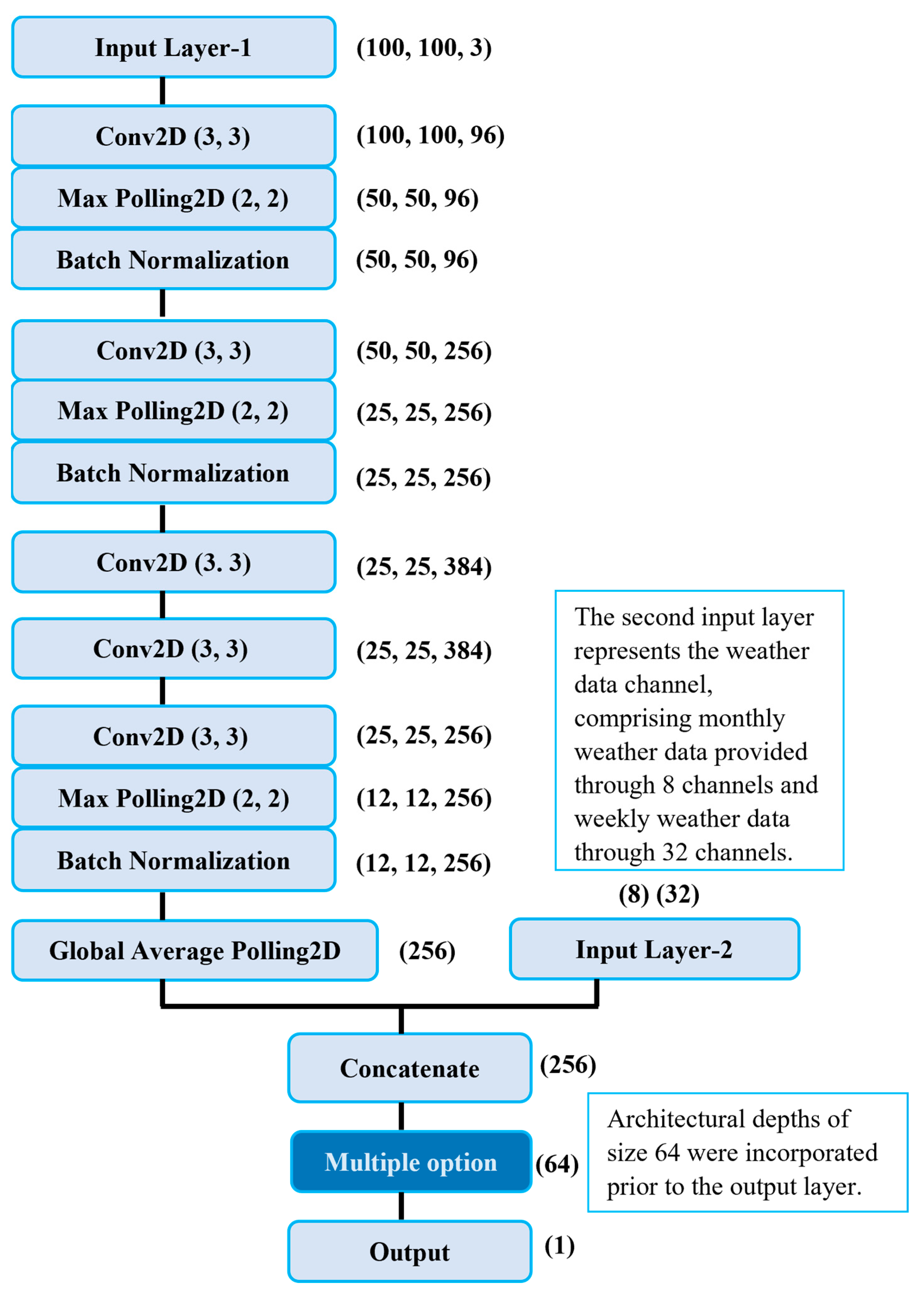
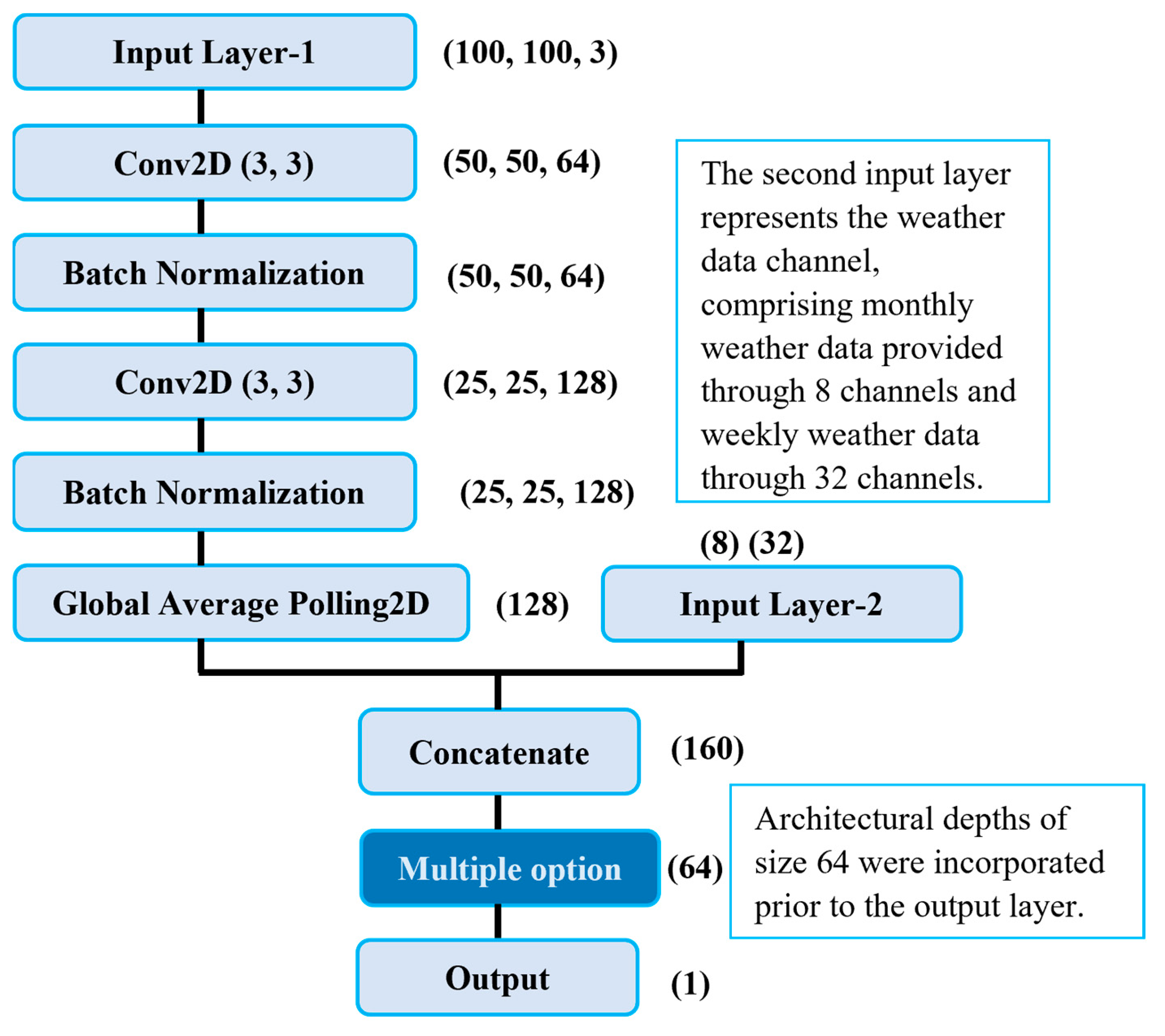
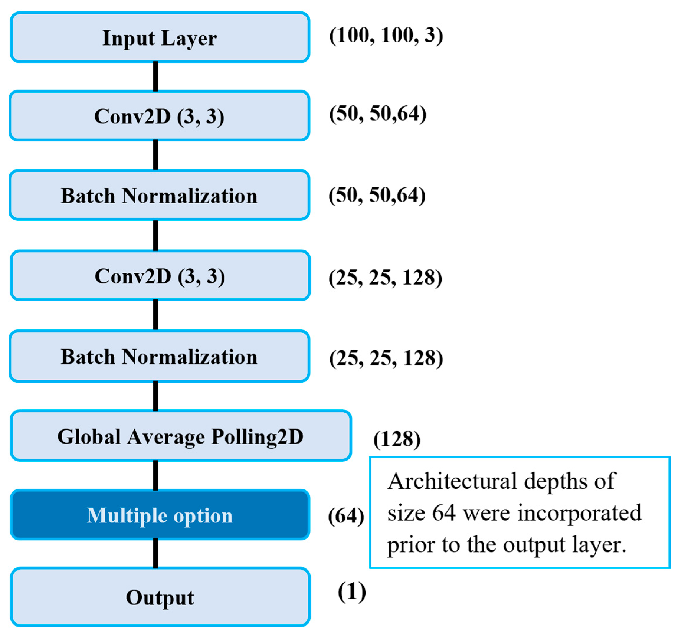
2.4. Neural Network Architectures

To obtain a robust and accurate yield prediction model, the architectures must be optimized based on the dataset. Two types of CNN feature extractor layers for multispectral images, three different depths of fully connected layers, and three methods of integrating weather data into deep neural network models were examined. The combinations created a total of 18 architectures to be compared. CNN architectures are primarily composed of convolutional layers and pooling layers. In the first layers, the model learns basic features and then builds on these basic features in subsequent layers. Two types of CNN layers are AlexNet and CNN_2conv. The AlexNet layer is a unique architecture that consists of five convolutional layers with the rectified linear unit (ReLU) function, three max pooling layers, and three fully connected layers [38]. However, the original AlexNet layer was modified in this study by adding three batch-normalization layers while removing three fully connected layers (Figure 2 and Figure 3). The CNN_2conv layer consists of two convolutional layers with two batch-normalization layers (Figure 4 and Figure 5). The input data for multispectral images had three channels, the red, green, and NIR channels, and three different UAV-based remote sensing platforms shared these bands. The three methods of integrating weather data into the CNN model were the inclusion of no weather data and the inclusion of weekly cumulative and monthly cumulative weather data collected after the heading stage. These weather data are one-dimensional vector data. Thus, weather data are concatenated with the output of the CNN layers (Figure 2 and Figure 4) and passed through the fully connected layers with different depths (Figure 2, Figure 3, Figure 4 and Figure 5). Finally, the output layer of the fully connected layer is fed to the output by a linear function (Figure 2, Figure 3, Figure 4 and Figure 5).
To assess the effectiveness of CNN layers, simple ANN was employed as a benchmark preliminary experiment. The ANN architectures are all the same as the above-mentioned CNN models (e.g., the number of layers, neurons, and activation functions) except that there is no CNN layer. Instead of the CNN layer, 100 pixels × 100 pixels image data of each band was averaged to reduce the dimensions of the input data. However, the performance of ANN was not stable and had substantially lower performance than the models based on the AlexNet and CNN_2conv architectures (Table S2). Thus, ANN was not included in further analysis.

2.5. Training and Validation Processes

All predictor variables underwent standardization (mean = 0 and standard deviation = 1) before the models were trained. The model performance was evaluated using fivefold cross-validation. For each fold, the entire dataset was randomly split into sets for training and testing the model: training (60%), validation (20%), and test (20%). To maintain consistency among the training, validation, and test datasets, the seed number was fixed among the models. The performance was measured using the R2, root mean squared error (RMSE), and root mean squared percentage error (RMSPE) values, which were calculated as follows:
R 2 = 1 i n y i y ^ i 2 i n y i y ¯ i 2
RMSE = i = 1 n y i y ^ i 2 n
RMSPE = 1 n i = 1 n y i y ^ i y i 2
where  y  and  y ^  are the observed and predicted yields, respectively,  i  is the sample number,  n  represents the total sample number, and  y ¯  represents the mean of the observed data. The mean  R 2 , RMSE, and RMSPE values were calculated from the five-fold results.
Data augmentation was applied to alleviate overfitting and improve the accuracy by increasing the total number of samples. The training dataset of multispectral images was augmented through buffer extraction, rotation, and flipping steps according to Tanabe et al. [24]. In the buffer extraction step, images were clipped at locations that moved one pixel away from the exact sampled location in the horizontal, vertical, and diagonal directions, thereby increasing the data size by nine times. The combination of the image rotation and flipping steps increased the data size by eight times. To avoid overfitting, these two augmentation methods were applied to the original images separately rather than simultaneously. In total, the original training dataset (n = 536) was multiplied sixteen times (n = 8576).
The CNN model training and testing process was performed in Python (version 3.8.10) using the Keras (version 2.8.0) machine learning application programming interface [39] with the TensorFlow (version 2.8.0) [40] backend. The Adam optimizer [38,41] was used with a learning rate of 0.001% (default value). To avoid overfitting, early stopping was used to monitor the validation loss with a patience of 15 epochs during a total of 100 epochs in the CNN models.
A randomly selected field (Field ID: 15) was utilized to forecast crop yields using the developed models. Yield prediction was performed based on 1.0 m × 1.0 m unit as same as input data of the yield prediction models. Yield prediction maps were visualized by gradient-colored points representing centroids of 1.0 m × 1.0 m prediction unit using QGIS 3.22.4. The chosen field was an on-farm experimental field where various fertilizer rates were used to cultivate the crops, and the average yield was 5.92 t ha−1. One of the best models from each combination was used for yield prediction, and the prediction time was recorded to evaluate the feasibility. The workstation specifications applied for these predictions were Intel Core i9-11900, Nvidia GTX 1650, 32.0 GB RAM, and Windows 10 64-bit system operation.

2.6. Statistical Analysis

Python (version 3.8.10) and SciPy (version 1.9.1) were used for the statistical analysis. Analysis of variance (ANOVA) was performed to evaluate the effects of architectures on the model performance. To examine the differences in the mean model performance values, Tukey’s honestly significant difference test (Tukey’s HSD) was performed. A p value < 0.05 was considered statistically significant for all analyses.

3. Results

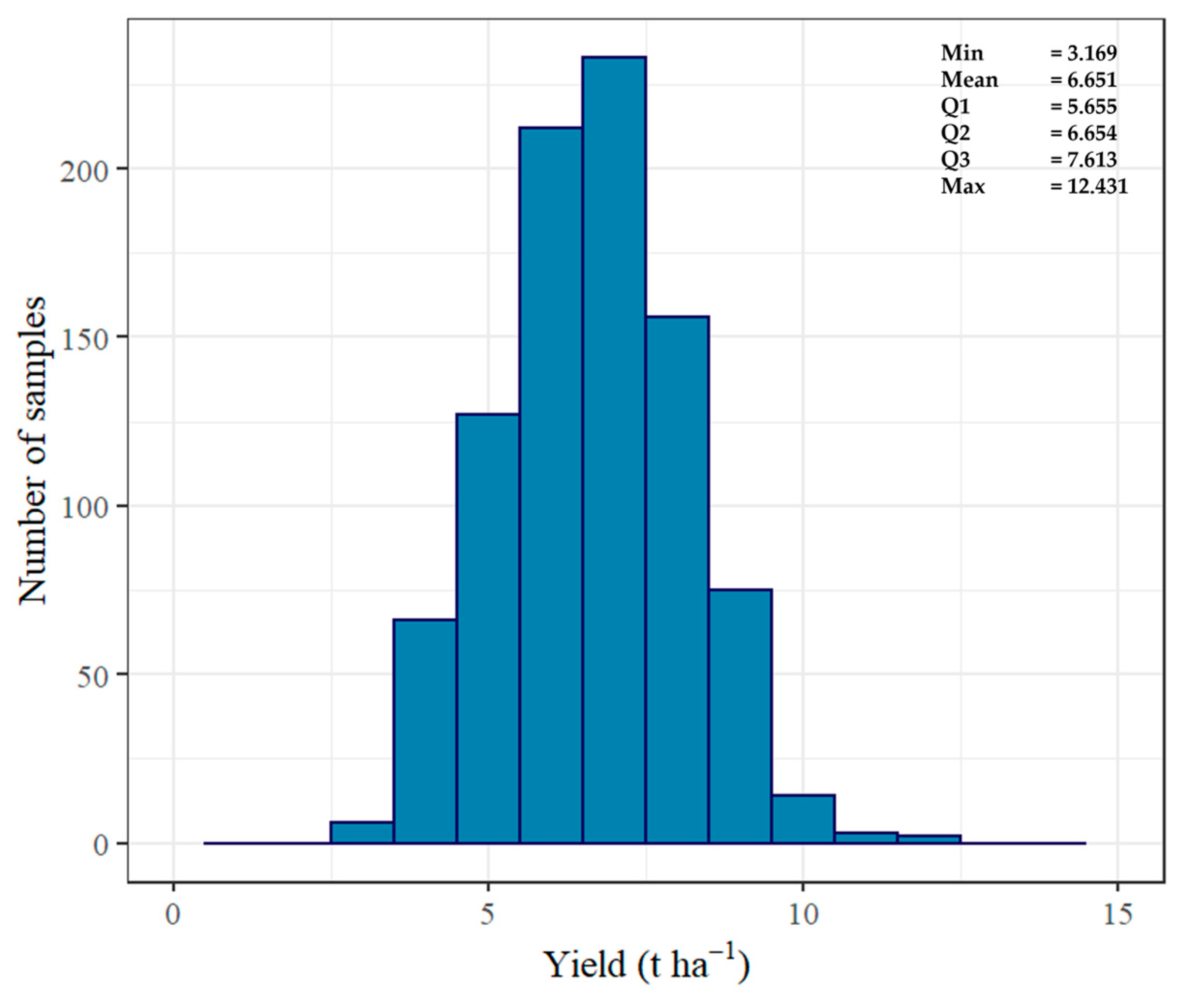
3.1. Yield Variations

A histogram of the yield data is shown in Figure 6. The collected data showed an approximately normal distribution, although there were a few extremely high-yield observations (>10 t ha−1, n = 894). The mean value was 6.65 t ha−1, and the standard deviation was 1.46 t ha−1 (coefficient of variation: 22.0%).

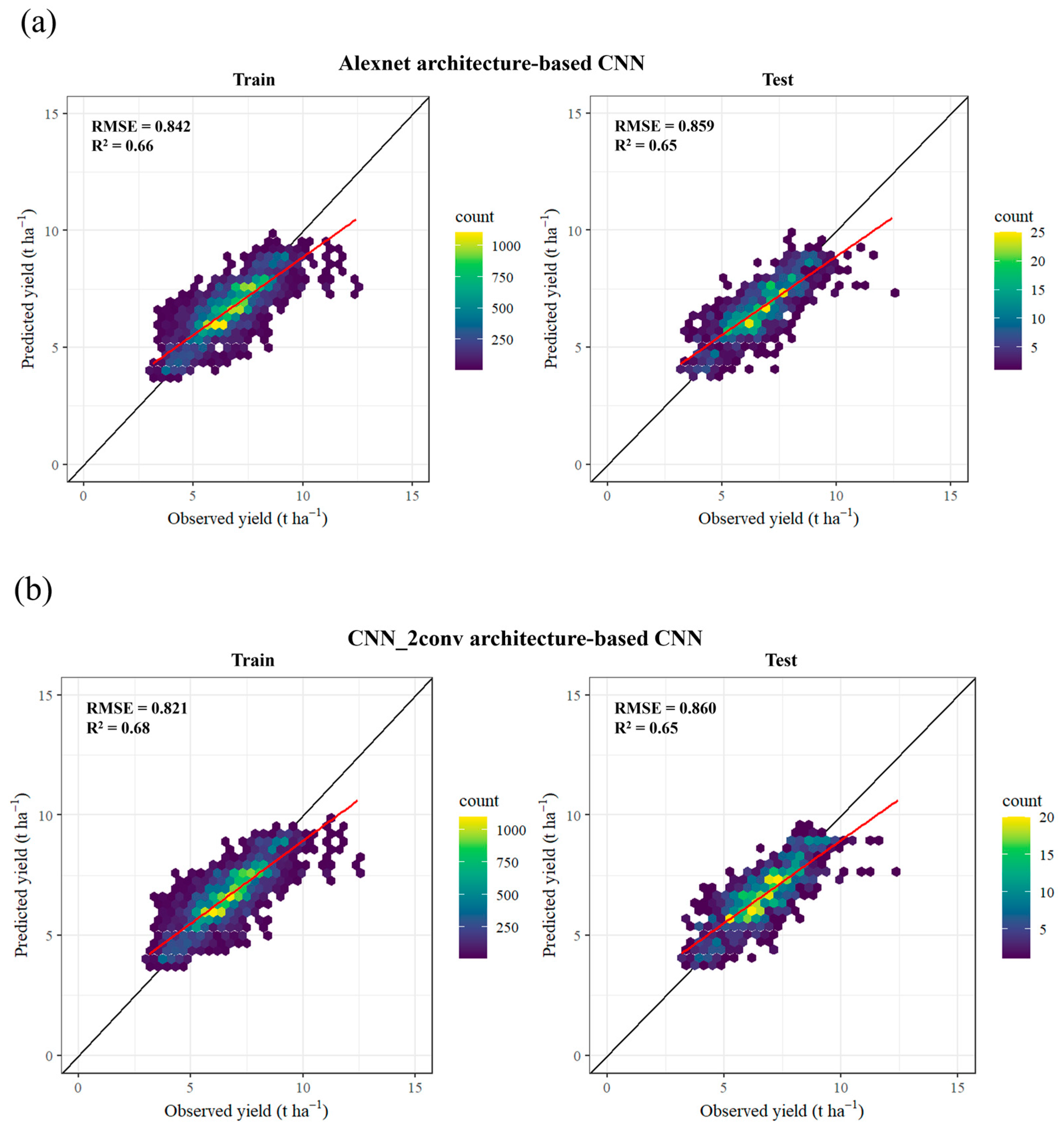
3.2. Model Performance

To assess the effects of the layer number, architecture, and weather data type on the RMSE, a three-way ANOVA was performed (Table 3). There was no significant difference between the AlexNet and CNN_2conv architectures. The effects of the number of layers and weather data types on the model performance were significant. However, there was no significant difference in the model performance among different layers according to Tukey’s HSD results. The models trained with weekly weather data exhibited significantly lower RMSE values than those trained with no weather and monthly weather data.
The performance of each model estimating the rice yield is presented in Table 4. Excluding the AlexNet models with no weather data (Models 1–3), the other models had high RMSE values when the layer depth was 0. The computational time required for prediction was approximately eight times longer in the AlexNet feature extractors than in the CNN_2conv ones. The top two accurate models with the lowest RMSE values were found in models integrating weekly weather data as input data with either AlexNet (Model 8) or CNN_2conv (Model 18). The relationships between the observed and predicted rice yields of the most accurate models, based on the AlexNet and CNN_2conv architecture-based models, are shown in Figure 7. There were no clear differences in the relationships between the observed and predicted yields when the AlexNet and CNN_2conv architecture-based models were compared.

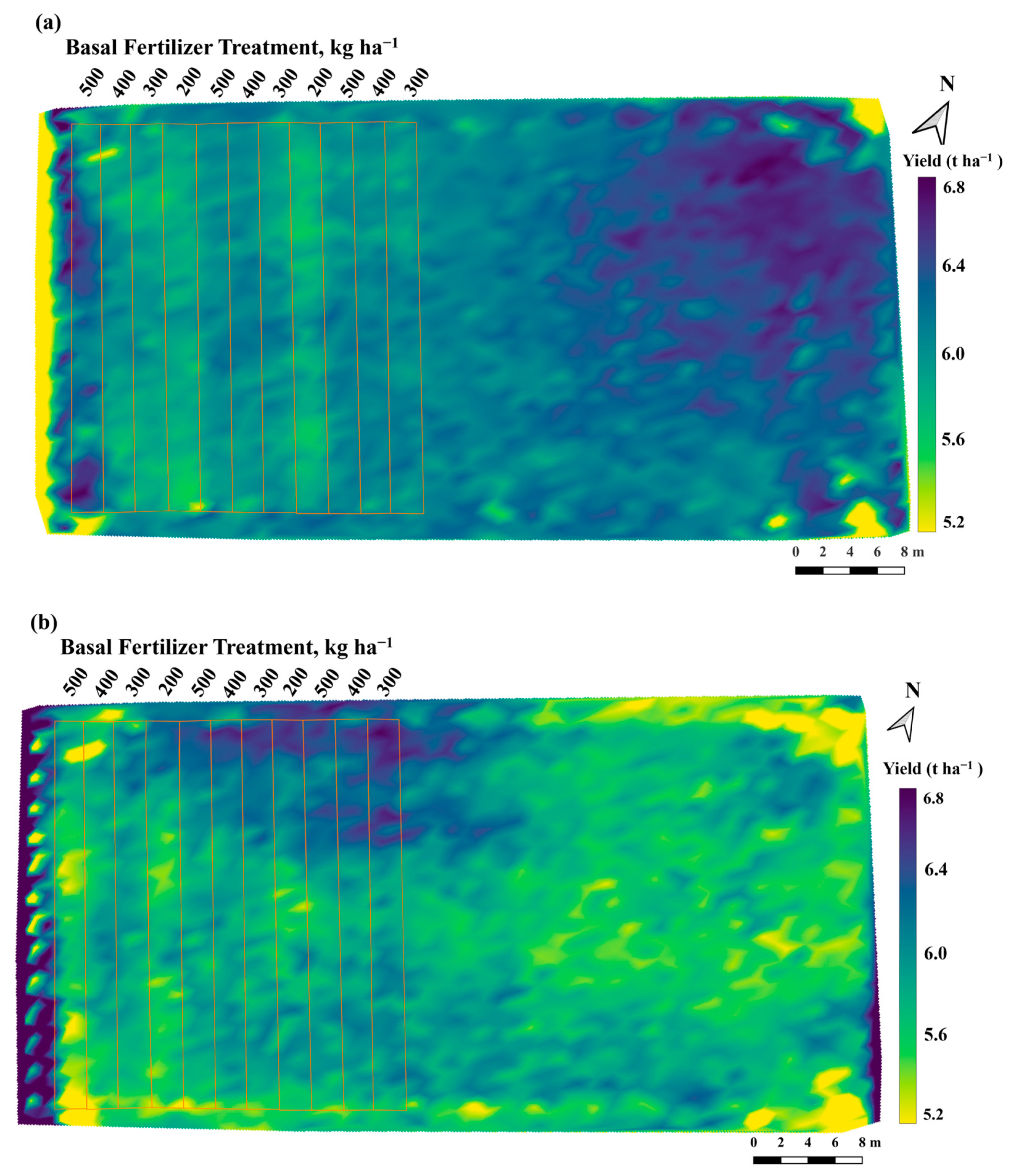
3.3. Within-Field Prediction of Rice Yield

The predicted yield maps based on the best models with both architectures (Models 8 and 18) are shown in Figure 8. Both predicted yield maps show spatially heterogenous yields (Figure 8 and Figure 9). The treatment plots receiving different rates of basal fertilizer were evident. The predicted yield range of the AlexNet architecture-based model (Model 8) was higher than that of the CNN_2conv architecture-based model (Model 18). The predicted yields ranged from 4.39 to 6.81 t ha−1 in Model 8 (mean value = 6.13 t ha−1), and from 4.11 to 679 t ha−1 in Model 18 (mean value = 5.82 t ha−1). The prediction yield maps, generated using the UAV-based optimal models of both architectures (Models 1 and 12), are depicted in Figure S1. Both models exhibit a nearly identical predicted pattern.

4. Discussion

This study attempted to explore the potential of multimodal deep learning models based on UAV multispectral and weather data to predict rice yields with high accuracy. The model performances were compared among different neural network architectures. The effects of the CNN feature extractor layers for multispectral images, depths of fully connected layers, and weather data integration methods on the model performance were examined. The results indicated that the best model could predict rice yields with an RMSE value of 0.859 t ha−1 (RMSPE: 14%) (Table 4; Figure 7). The architecture of this model consisted of an AlexNet feature extractor, weekly weather data, and one layer after concatenation (Model 8). Moreover, the second-best model could predict rice yields with an RMSE value of 0.860 t ha−1 (RMSPE: 14%). The architecture of this model consisted of a CNN_2conv feature extractor, weekly weather data, and two layers after concatenation (Model 18). These two best models indicated that multimodal deep neural network models based on UAV multispectral imagery and weekly aggregated data might contribute to the enhancement of prediction accuracies. The result of Tukey’s HSD also showed that the use of weekly weather data resulted in significantly lower RMSEs than using no weather data (Table 3). This finding was consistent with previous studies reporting that the crop yield prediction accuracy obtained based on satellite imagery could be enhanced by integrating weather data [31,32,42]. Notably, UAV-based approaches may provide more homogenous climate data for each observation than satellite-based approaches because the spatial resolution of available weather data is relatively coarse (1 km2) compared to the relatively spatially fine resolutions and limited regions of interest of UAV-based remote sensing data. For instance, a single field, or even adjacent fields, shared identical weather data values in this study. Despite the inevitable nature of unbalanced training-data sampling for UAV-based approaches, the integration of weekly weather data is important for improving within-field yield prediction accuracies. However, monthly cumulative weather data did not significantly improve the model performance (Table 3). The results indicated that appropriate temporal intervals for aggregating weather data should be explored in future studies. Deep learning models consisting of RNN or long short-term memory (LSTM) layers for extracting the temporal features of weather data can contribute to improving the model prediction accuracy in crop yield predictions [43].
One of the key aspects of CNNs is their high capability to extract spatial features; this capability is enabled by the deep and complicated architectures of these networks. Therefore, deeper networks can learn more complex spatial features from the input data, which might improve the accuracy and robustness of the prediction model [22,42,44]. In the present study, the AlexNet feature extractor was assumed to outperform the CNN_2conv feature extractor due to its architectural complexity. However, the spatial feature extractors had no significant effect on the model performance (Table 3). Little difference was found in the model performance between the two best models (Models 8 and 18) (Table 4). Furthermore, the CNN_2conv feature extractor was eight times more efficient than the AlexNet feature extractor in terms of the computation time (Table 4). Therefore, the results indicated that the CNN architectural complexity might not be essential from the perspective of the prediction accuracy, but computational feasibility of the model should be accounted in practical applications.
To present an efficient paradigm design architecture for multimodal deep learning models, the effect of additional layers after the concatenation of outputs from CNN layers and weather data on the model performance was also evaluated. The three-way ANOVA test indicated a significant effect of the number of layers on the model performance (Table 3). The RMSE values decreased with an increasing number of layers, although there was no significant difference according to the result of Tukey’s HSD (Table 3). The best two models (Models 8 and 18) had more than one layer after the concatenation of weather data (Table 4). Therefore, adding at least one extra layer to the architectures, just after concatenating the spatial data extracted by CNN layers and temporal weather data, could lead to an improvement in the modeling accuracy. Accordingly, the nonlinear relationships realized from spatial (i.e., multispectral images) and temporal information (i.e., weather data) can be efficiently used to predict yields.
Although both best models (Models 8 and 18) exhibited similar prediction accuracies (Table 4; Figure 7), the predicted yield levels and spatial patterns varied between them (Figure 8). Specifically, Model 8 predicted a higher yield range than Model 18. Furthermore, Model 18 predicted lower yields than Model 8 in the northeastern part of the field, while near the northern boundary, where Model 18 predicted higher yields, Model 8 predicted lower yields. On the edges of the east and west sides of the field, Model 8 predicted lower yields, while Model 18 predicted extremely high yields. The effects of the fertilizer treatments on the predicted yields were more evident in Model 8 than in Model 18. Both models similarly predicted extremely high and low values, but values near the median showed high variations (Figure 9). When a practitioner selected different models, the resultant yield maps varied substantially. Yield data are basic information used for data analytics in on-farm experiments to evaluate the effects of treatments on the crop yield [45]. Therefore, there is a risk that different scenarios could be derived depending on which model is used for the yield prediction and further data analytics in on-farm experimentations to provide fertilization recommendations, although there were apparently no significant differences in the yield prediction accuracies in this study. The results indicated that not only the prediction accuracy, but also the robustness of the within-field yield predictions, should be assessed in further studies.
Although this study indicated that integrating weekly weather data into CNN models could contribute to enhancing yield prediction accuracy, several limitations should be noted. Weather data were uniformly distributed across the adjacent fields due to the spatial resolution of database (i.e., 1 km × 1 km). If there are more spatial and temporal variations in weather data for each field, the impact of time-series data algorithms, such as recurrent neural network and LSTM, on model performance should be assessed using daily weather data in further research. Furthermore, this study could not identify which models were the most reliable and robust, as indicated by the different spatial yield distributions between models (Figure 7 and Figure 8). The results highlighted an important finding; namely, that models could differently predict spatial variations even with almost the same prediction accuracy. Thus, further studies are required to evaluate site-specific prediction accuracy using independent field test datasets with more spatially dense observations (i.e., yield monitor data).

5. Conclusions

This study indicated that a multimodal deep learning model integrating UAV-based multispectral imagery and weather data has the potential to develop more precise rice yield predictions. The results highlighted that the best models were trained with weekly weather data. A simple CNN feature extractor for UAV-based multispectral image input data might be sufficient to predict crop yields accurately. However, the yield levels and spatial patterns of the predicted yield map differed among models, although the prediction accuracy was almost the same. Further research will be required to explore the robustness of this approach by collecting a variety of yield observations alongside weather data.

Supplementary Materials

The following supporting information can be downloaded at: https://www.mdpi.com/article/10.3390/rs15102511/s1, Figure S1: Yield prediction maps (using only UAV images) of a surveyed field based on (a) Model 1 and (b) Model 12; Table S1: Weekly and monthly summation of mean air temperature, solar radiation, and total precipitation for four weeks after heading stage at the study sites; Table S2: ANN model performance for predicting rice yields with the training, validation, and test datasets.

Author Contributions

Conceptualization, T.S.T.T.; methodology, M.S.M., R.T. and T.S.T.T.; software, M.S.M., R.T. and T.S.T.T.; validation, M.S.M. and T.S.T.T.; formal analysis, M.S.M. and L.N.H.; investigation, M.S.M., L.N.H., N.H., K.H., M.M. and T.S.T.T.; resources, M.S.M., N.H., K.H., M.M. and T.S.T.T.; data curation, M.S.M.; writing—original draft preparation, M.S.M.; writing—review and editing, T.S.T.T.; visualization, M.S.M., L.N.H. and T.S.T.T.; supervision, T.M.; project administration, T.S.T.T.; funding acquisition, T.S.T.T. All authors have read and agreed to the published version of the manuscript.

Funding

This research was funded by the Japan Science and Technology Agency (JST), ACT-X, grant number JPMJAX20AF.

Data Availability Statement

Data will be made available on request.

Acknowledgments

The authors wish to thank the farmers who allowed survey of their fields.

Conflicts of Interest

The authors declare no conflict of interest.

References

  1. Nyéki, A.; Neményi, M. Crop Yield Prediction in Precision Agriculture. Agronomy 2022, 12, 2460. [Google Scholar] [CrossRef]
  2. Mariotto, I.; Thenkabail, P.S.; Huete, A.; Slonecker, E.T.; Platonov, A. Hyperspectral versus Multispectral Crop-Productivity Modeling and Type Discrimination for the HyspIRI Mission. Remote Sens. Environ. 2013, 139, 291–305. [Google Scholar] [CrossRef]
  3. Wang, L.; Tian, Y.; Yao, X.; Zhu, Y.; Cao, W. Predicting Grain Yield and Protein Content in Wheat by Fusing Multi-Sensor and Multi-Temporal Remote-Sensing Images. Field Crops Res. 2014, 164, 178–188. [Google Scholar] [CrossRef]
  4. Zhou, X.; Kono, Y.; Win, A.; Matsui, T.; Tanaka, T.S.T. Predicting Within-Field Variability in Grain Yield and Protein Content of Winter Wheat Using UAV-Based Multispectral Imagery and Machine Learning Approaches. Plant Prod. Sci. 2021, 24, 137–151. [Google Scholar] [CrossRef]
  5. Han, X.; Liu, F.; He, X.; Ling, F. Research on Rice Yield Prediction Model Based on Deep Learning. Comput. Intell. Neurosci. 2022, 2022, 1922561. [Google Scholar] [CrossRef]
  6. Cao, J.; Zhang, Z.; Tao, F.; Zhang, L.; Luo, Y.; Zhang, J.; Han, J.; Xie, J. Integrating Multi-Source Data for Rice Yield Prediction across China Using Machine Learning and Deep Learning Approaches. Agric. For. Meteorol. 2021, 297, 108275. [Google Scholar] [CrossRef]
  7. Cai, Y.; Guan, K.; Lobell, D.; Potgieter, A.B.; Wang, S.; Peng, J.; Xu, T.; Asseng, S.; Zhang, Y.; You, L.; et al. Integrating Satellite and Climate Data to Predict Wheat Yield in Australia Using Machine Learning Approaches. Agric. Meteorol. 2019, 274, 144–159. [Google Scholar] [CrossRef]
  8. Haghighat, A.K.; Ravichandra-Mouli, V.; Chakraborty, P.; Esfandiari, Y.; Arabi, S.; Sharma, A. Applications of Deep Learning in Intelligent Transportation Systems. J. Big Data Anal. Transp. 2020, 2, 115–145. [Google Scholar] [CrossRef]
  9. Srivastava, A.K.; Safaei, N.; Khaki, S.; Lopez, G.; Zeng, W.; Ewert, F.; Gaiser, T.; Rahimi, J. Winter Wheat Yield Prediction Using Convolutional Neural Networks from Environmental and Phenological Data. Sci. Rep. 2022, 12, 3215. [Google Scholar] [CrossRef]
  10. Fieuzal, R.; Marais Sicre, C.; Baup, F. Estimation of Corn Yield Using Multi-Temporal Optical and Radar Satellite Data and Artificial Neural Networks. Int. J. Appl. Earth Obs. Geoinf. 2017, 57, 14–23. [Google Scholar] [CrossRef]
  11. Amaratunga, V.; Wickramasinghe, L.; Perera, A.; Jayasinghe, J.; Rathnayake, U. Artificial Neural Network to Estimate the Paddy Yield Prediction Using Climatic Data. Math. Probl. Eng. 2020, 2020, 8627824. [Google Scholar] [CrossRef]
  12. Aghighi, H.; Azadbakht, M.; Ashourloo, D.; Shahrabi, H.S.; Radiom, S. Machine Learning Regression Techniques for the Silage Maize Yield Prediction Using Time-Series Images of Landsat 8 OLI. IEEE J. Sel. Top. Appl. Earth Obs. Remote Sens. 2018, 11, 4563–4577. [Google Scholar] [CrossRef]
  13. Jeong, J.H.; Resop, J.P.; Mueller, N.D.; Fleisher, D.H.; Yun, K.; Butler, E.E.; Timlin, D.J.; Shim, K.-M.; Gerber, J.S.; Reddy, V.R.; et al. Random Forests for Global and Regional Crop Yield Predictions. PLoS ONE 2016, 11, e0156571. [Google Scholar] [CrossRef] [PubMed]
  14. Prasad, N.R.; Patel, N.R.; Danodia, A. Crop Yield Prediction in Cotton for Regional Level Using Random Forest Approach. Spat. Inf. Res. 2021, 29, 195–206. [Google Scholar] [CrossRef]
  15. Jui, S.J.J.; Ahmed, A.A.M.; Bose, A.; Raj, N.; Sharma, E.; Soar, J.; Chowdhury, M.W.I. Spatiotemporal Hybrid Random Forest Model for Tea Yield Prediction Using Satellite-Derived Variables. Remote Sens. 2022, 14, 805. [Google Scholar] [CrossRef]
  16. Liu, Y.; Wang, S.; Wang, X.; Chen, B.; Chen, J.; Wang, J.; Huang, M.; Wang, Z.; Ma, L.; Wang, P.; et al. Exploring the Superiority of Solar-Induced Chlorophyll Fluorescence Data in Predicting Wheat Yield Using Machine Learning and Deep Learning Methods. Comput. Electron. Agric. 2022, 192, 106612. [Google Scholar] [CrossRef]
  17. Kuwata, K.; Shibasaki, R. Estimating Corn Yield in the United States with Modis Evi and Machine Learning Methods. ISPRS Ann. Photogramm. Remote Sens. Spat. Inf. Sci. 2016, III-8, 131–136. [Google Scholar] [CrossRef]
  18. Wang, K.; Franklin, S.E.; Guo, X.; Cattet, M. Remote Sensing of Ecology, Biodiversity and Conservation: A Review from the Perspective of Remote Sensing Specialists. Sensors 2010, 10, 9647–9667. [Google Scholar] [CrossRef]
  19. Maimaitijiang, M.; Sagan, V.; Sidike, P.; Hartling, S.; Esposito, F.; Fritschi, F.B. Soybean Yield Prediction from UAV Using Multimodal Data Fusion and Deep Learning. Remote Sens. Environ. 2020, 237, 111599. [Google Scholar] [CrossRef]
  20. Zhou, J.; Lu, X.; Yang, R.; Chen, H.; Wang, Y.; Zhang, Y.; Huang, J.; Liu, F. Developing Novel Rice Yield Index Using UAV Remote Sensing Imagery Fusion Technology. Drones 2022, 6, 151. [Google Scholar] [CrossRef]
  21. Fu, Z.; Yu, S.; Zhang, J.; Xi, H.; Gao, Y.; Lu, R.; Zheng, H.; Zhu, Y.; Cao, W.; Liu, X. Combining UAV Multispectral Imagery and Ecological Factors to Estimate Leaf Nitrogen and Grain Protein Content of Wheat. Eur. J. Agron. 2022, 132, 126405. [Google Scholar] [CrossRef]
  22. Tanabe, R.; Matsui, T.; Tanaka, T.S.T. Winter Wheat Yield Prediction Using Convolutional Neural Networks and UAV-Based Multispectral Imagery. Field Crops Res. 2023, 291, 108786. [Google Scholar] [CrossRef]
  23. Yang, Q.; Shi, L.; Han, J.; Zha, Y.; Zhu, P. Deep Convolutional Neural Networks for Rice Grain Yield Estimation at the Ripening Stage Using UAV-Based Remotely Sensed Images. Field Crops Res. 2019, 235, 142–153. [Google Scholar] [CrossRef]
  24. Wang, F.; Wang, F.; Zhang, Y.; Hu, J.; Huang, J.; Xie, J. Rice Yield Estimation Using Parcel-Level Relative Spectral Variables from UAV-Based Hyperspectral Imagery. Front. Plant Sci. 2019, 10, 453. [Google Scholar] [CrossRef] [PubMed]
  25. Long, J.; Shelhamer, E.; Darrell, T. Fully Convolutional Networks for Semantic Segmentation. In Proceedings of the 2015 IEEE Conference on Computer Vision and Pattern Recognition (CVPR), Boston, MA, USA, 7–12 June 2015; IEEE: New York, NY, USA, 2015; pp. 3431–3440. [Google Scholar]
  26. Collobert, R.; Weston, J. A Unified Architecture for Natural Language Processing: Deep Neural Networks with Multitask Learning. In Proceedings of the 25th International Conference on Machine Learning, New York, NY, USA, 5–9 July 2008. [Google Scholar]
  27. Ji, S.; Xu, W.; Yang, M.; Yu, K. 3D Convolutional Neural Networks for Human Action Recognition. IEEE Trans. Pattern Anal. Mach. Intell. 2012, 35, 221–231. [Google Scholar] [CrossRef]
  28. Sinclair, T.R.; Horie, T. Leaf Nitrogen, Photosynthesis, and Crop Radiation Use Efficiency: A Review. Crop. Sci. 1989, 29, 90–98. [Google Scholar] [CrossRef]
  29. Yoshimoto, M.; Fukuoka, M.; Tsujimoto, Y.; Matsui, T.; Kobayasi, K.; Saito, K.; van Oort, P.A.J.; Inusah, B.I.Y.; Vijayalakshmi, C.; Vijayalakshmi, D.; et al. Monitoring Canopy Micrometeorology in Diverse Climates to Improve the Prediction of Heat-Induced Spikelet Sterility in Rice under Climate Change. Agric. Meteorol. 2022, 316, 108860. [Google Scholar] [CrossRef]
  30. Song, Y.; Wang, J.; Wang, L. Satellite Solar-Induced Chlorophyll Fluorescence Reveals Heat Stress Impacts on Wheat Yield in India. Remote Sens. 2020, 12, 3277. [Google Scholar] [CrossRef]
  31. Jiang, D.; Yang, X.; Clinton, N.; Wang, N. An Artificial Neural Network Model for Estimating Crop Yields Using Remotely Sensed Information. Int. J. Remote Sens. 2004, 25, 1723–1732. [Google Scholar] [CrossRef]
  32. Kim, N.; Lee, Y.-W. Machine Learning Approaches to Corn Yield Estimation Using Satellite Images and Climate Data: A Case of Iowa State. J. Korean Soc. Surv. Geod. Photogramm. Cartogr. 2016, 34, 383–390. [Google Scholar] [CrossRef]
  33. Alzubaidi, L.; Zhang, J.; Humaidi, A.J.; Al-Dujaili, A.; Duan, Y.; Al-Shamma, O.; Santamaría, J.; Fadhel, M.A.; Al-Amidie, M.; Farhan, L. Review of Deep Learning: Concepts, CNN Architectures, Challenges, Applications, Future Directions. J. Big Data 2021, 8, 53. [Google Scholar] [CrossRef] [PubMed]
  34. Qian, W.; Kang, H.S.; Lee, D.K. Distribution of seasonal rainfall in the East Asian monsoon region. Theor. Appl. Climatol. 2002, 73, 151–168. [Google Scholar] [CrossRef]
  35. Kanda, T.; Takata, Y.; Kohayama, K.; Ohkura, T.; Maejima, Y.; Wakabayashi, S.; Obara, H. New Soil Maps of Japan based on the Comprehensive Soil Classification System of Japan—First Approximation and its Application to the World Reference Base for Soil Resources 2006. Jpn. Agric. Res. Q. (JARQ) 2018, 52, 285–292. Available online: https://www.jstage.jst.go.jp/article/jarq/52/4/52_285 (accessed on 5 April 2023). [CrossRef]
  36. Ohno, H.; Sasaki, K.; Ohara, G.; Nakazono, K. Development of Grid Square Air Temperature and Precipitation Data Compiled from Observed, Forecasted, and Climatic Normal Data. Clim. Biosph. 2016, 16, 71–79. [Google Scholar] [CrossRef]
  37. Luo, S.; Jiang, X.; Jiao, W.; Yang, K.; Li, Y.; Fang, S. Remotely Sensed Prediction of Rice Yield at Different Growth Durations Using UAV Multispectral Imagery. Agriculture 2022, 12, 1447. [Google Scholar] [CrossRef]
  38. Krizhevsky, A.; Sutskever, I.; Hinton, G.E. ImageNet Classification with Deep Convolutional Neural Networks. Commun. ACM 2017, 60, 84–90. [Google Scholar] [CrossRef]
  39. Hinton, G.E.; Srivastava, N.; Krizhevsky, A.; Sutskever, I.; Salakhutdinov, R.R. Improving Neural Networks by Preventing Co-Adaptation of Feature Detectors. arXiv 2012, arXiv:1207.0580. [Google Scholar]
  40. Abadi, M.; Agarwal, A.; Barham, P.; Brevdo, E.; Chen, Z.; Citro, C.; Corrado, G.S.; Davis, A.; Dean, J.; Devin, M.; et al. TensorFlow: Large-Scale Machine Learning on Heterogeneous Distributed Systems. arXiv 2016, arXiv:1603.04467. [Google Scholar]
  41. Kingma, D.P.; Ba, J. Adam: A Method for Stochastic Optimization. arXiv 2014, arXiv:1412.6980. [Google Scholar]
  42. Huang, H.; Huang, J.; Feng, Q.; Liu, J.; Li, X.; Wang, X.; Niu, Q. Developing a Dual-Stream Deep-Learning Neural Network Model for Improving County-Level Winter Wheat Yield Estimates in China. Remote Sens. 2022, 14, 5280. [Google Scholar] [CrossRef]
  43. Shook, J.; Gangopadhyay, T.; Wu, L.; Ganapathysubramanian, B.; Sarkar, S.; Singh, A.K. Crop Yield Prediction Integrating Genotype and Weather Variables Using Deep Learning. PLoS ONE 2021, 16, e0252402. [Google Scholar] [CrossRef] [PubMed]
  44. Gavahi, K.; Abbaszadeh, P.; Moradkhani, H. DeepYield: A Combined Convolutional Neural Network with Long Short-Term Memory for Crop Yield Forecasting. Expert. Syst. Appl. 2021, 184, 115511. [Google Scholar] [CrossRef]
  45. Tanaka, T.S.T. Assessment of Design and Analysis Frameworks for On-Farm Experimentation through a Simulation Study of Wheat Yield in Japan. Precis. Agric. 2021, 22, 1601–1616. [Google Scholar] [CrossRef]
Figure 1. Images captured through UAV and multispectral cameras of different bands in a 1.0 m × 1.0 m area: (a) green, (b) NIR (near-infrared), and (c) red. The legend represents reflectance values.
Remotesensing 15 02511 g001
Figure 2. The AlexNet architecture-based CNN model with weather data. The numbers next to the boxes are the output shapes of the indicated layers.
Remotesensing 15 02511 g002
Figure 3. The AlexNet architecture-based CNN model without weather data. The numbers next to the boxes are the output shapes of the indicated layers.
Remotesensing 15 02511 g003
Figure 4. The CNN-2conv architecture-based CNN model with weather data. The numbers next to the boxes are the output shapes of the indicated layers.
Remotesensing 15 02511 g004
Figure 5. The CNN-2conv architecture-based CNN model without weather data. The numbers next to the boxes are the output shapes of the indicated layers.
Remotesensing 15 02511 g005
Figure 6. Histogram of all yield observations (n = 894; Q1, 25th percentile; Q2, median quartile; Q3, 75th percentile).
Remotesensing 15 02511 g006
Figure 7. Relationships between the observed and predicted grain yields derived from (a) Model 8 and (b) Model 18 with the training and test datasets.
Remotesensing 15 02511 g007
Figure 8. Yield prediction maps of a surveyed field based on (a) Model 8 and (b) Model 18.
Remotesensing 15 02511 g008
Figure 9. Scatter plot of predicted yield by Model 8 vs. Model 18 for a selected field (Field ID: 15). The red line indicates the 1:1 line.
Remotesensing 15 02511 g009
Table 1. Basic information on the research fields. The same letter of Environment ID represents locations having the same weather dataset.
Field IDPrefectureLatitudeLongitudeEnvironment IDSowing/Transplanting DatePlanting SystemUav Imagery
Acquisition Date
VarietyCamera
01Miyagi38°13′N140°58′EA25 April 2017Direct Seeding2 August 2017HitomeboreSequoia+
02Miyagi38°13′N140°58′EA7 May 2017Transplanting2 August 2017HitomeboreSequoia+
03Miyagi38°13′N140°58′EB29 April 2018Direct Seeding2 August 2018ManamusumeSequoia+
04Miyagi38°13′N140°58′EB7 May 2018Transplanting2 August 2018HitomeboreSequoia+
05Miyagi38°12′N140°58′EC4 May 2019Direct Seeding8 August 2019HitomeboreSequoia+
06Miyagi38°13′N140°58′EC12 May 2019Transplanting8 August 2019HitomeboreSequoia+
07Miyagi38°13′N140°58′EC16 May 2019Transplanting8 August 2019HitomeboreSequoia+
08Gifu35°38′N137°06′ED11 May 2020Transplanting12 August 2020KoshihikariRededge Altum
09Gifu35°13′N136°40′EE11 May 2020Transplanting6 August 2020KoshihikariRededge Altum
10Gifu35°14′N136°35′EF11 May 2020Transplanting6 August 2020HoshijirushiRededge Altum
11Gifu35°15′N136°35′EG23 May 2020Transplanting6 August 2020HoshijirushiRededge Altum
12Gifu35°15′N136°35′EH25 April 2021Transplanting13 July 2021AkitakomachiRededge Altum
13Gifu35°14′N136°35′EH19 April 2021Transplanting13 July 2021ShikiyutakaRededge Altum
14Gifu35°15′N136°35′EI14 May 2021Transplanting11 August 2021HoshijirushiRededge Altum
15Gifu35°11′N136°38′EJ10 May 2021Transplanting11 August 2021HoshijirushiRededge Altum
16Gifu35°13′N136°40′EK11 May 2021Transplanting11 August 2021HoshijirushiRededge Altum
17Gifu35°15′N136°35′EL16 May 2022Transplanting9 August 2022HoshijirushiRededge Altum
18Gifu35°16′N136°35′EM23 May 2022Transplanting9 August 2022HoshijirushiRededge Altum
19Gifu35°14′N136°39′EM2 May 2022Transplanting9 August 2022HoshijirushiRededge Altum
20Kochi33°35′N133°38′EN31 March 2022Transplanting1 July 2022Nangoku SodachiP4 Multispectral
21Kochi33°35′N133°38′EO4 April 2022Transplanting1 July 2022Yosakoi bijinP4 Multispectral
22Kochi33°35′N133°39′EO25 May 2022Transplanting29 July 2022KoshihikariP4 Multispectral
Same letter indicates same environment.
Table 2. The specs of multispectral cameras.
CameraSpectral Band Width
(nm)
Field of View
(H × V)
Resolution (Pixel)
GreenRedNear Infrared (NIR)
Sequoia+550 ± 40660 ± 40790 ± 4062 × 2491280 × 960
Rededge Altum560 ± 27668 ± 14842 ± 5748 × 372064 × 1544
P4 Multispectral560 ± 16650 ± 16840 ± 2662.7 × 62.71600 × 1300
Table 3. Result of three-way ANOVA on the layer numbers, weather data types, and architectures.
RMSE
t ha−1
Layer
00.933 a
10.910 a
20.898 a
Weather
No0.941 a
Monthly0.917 a
Weekly0.877 b
Architecture
AlexNet0.909 a
CNN_2conv0.910 a
ANOVAp value
Layer0.024
Weather0.003
Architecturen.s
Layer × Weathern.s
Layer × Architecturen.s
Weather × Architecturen.s
Different small letters within each column indicate significant differences at a p-value < 0.05 according to Tukey’s HSD test. n.s., not significant.
Table 4. CNN model performance for predicting rice yields with the training, validation, and test datasets.
Model No.ArchitectureWeatherLayerTrainValidationTestTime for Prediction
RMSERMSPER2RMSERMSPER2RMSERMSPER2
t ha−1% t ha−1% t ha−1% s/ha
1AlexNetNo00.985160.540.867150.650.929150.5925.91
2AlexNetNo10.986150.540.908160.620.948150.5725.75
3AlexNetNo20.964150.560.882150.640.940160.5825.69
4AlexNetMonthly00.953150.570.897160.630.917150.6025.67
5AlexNetMonthly10.938150.580.869150.650.920150.5925.53
6AlexNetMonthly20.905150.610.862150.650.897150.6125.82
7AlexNetWeekly00.897150.620.859150.650.905150.6125.56
8AlexNetWeekly10.842140.660.830150.680.859140.6525.69
9AlexNetWeekly20.839140.670.845150.670.868140.6425.75
10CNN_2convNo01.045170.480.912160.610.969160.553.29
11CNN_2convNo11.024160.500.894150.630.931150.583.24
12CNN_2convNo20.978150.550.893150.630.929150.593.25
13CNN_2convMonthly00.998160.530.916160.610.970160.553.32
14CNN_2convMonthly10.906140.610.877150.640.905150.613.52
15CNN_2convMonthly20.905140.610.876150.640.895150.623.16
16CNN_2convWeekly00.905150.610.857150.660.907150.602.21
17CNN_2convWeekly10.833130.670.834140.680.864140.643.20
18CNN_2convWeekly20.821130.680.831140.680.860140.653.22
Bold letters represent the best model based on the model performance with the training, validation, and test datasets.
Disclaimer/Publisher’s Note: The statements, opinions and data contained in all publications are solely those of the individual author(s) and contributor(s) and not of MDPI and/or the editor(s). MDPI and/or the editor(s) disclaim responsibility for any injury to people or property resulting from any ideas, methods, instructions or products referred to in the content.

