Article

Monitoring Seasonal Movement Characteristics of the Landslide Based on Time-Series InSAR Technology: The Cheyiping Landslide Case Study, China

1
Key Laboratory of Digital Earth Science, Aerospace Information Research Institute, Chinese Academy of Sciences, Beijing 100094, China
2
International Research Center of Big Data for Sustainable Development Goals, Beijing 100094, China
3
University of Chinese Academy of Sciences, Beijing 100049, China
*
Author to whom correspondence should be addressed.
Remote Sens. 2023, 15(1), 51; https://doi.org/10.3390/rs15010051
Submission received: 28 September 2022 / Revised: 17 December 2022 / Accepted: 19 December 2022 / Published: 22 December 2022

Abstract

:
Landslides are one of the extremely high-incidence and serious-loss geological disasters in the world, and the early monitoring and warning of landslides are of great importance. The Cheyiping landslide, located in western Yunnan Province, China, added many cracks and dislocations to the surface of the slope due to the severe seasonal rainfall and rise of the water level, which seriously threaten the safety of residents and roads located on the body and foot of the slope. To investigate the movement of the landslide, this paper used Sentinel-1A SAR data processed by time-series interferometric synthetic aperture radar (InSAR) technology to monitor the long-time surface deformation. The landslide boundary was defined, then the spatial distribution of landslide surface deformation from 5 January 2018 to 27 December 2021 was obtained. According to the monthly rainfall data and the temporal deformation results, the movement of the landslide was highly correlated with seasonal rainfall, and the Cheyiping landslide underwent seasonal sectional accelerated deformation. Moreover, the water level change of the Lancang River caused by the water storage of the hydropower station and seasonal rainfall accelerates the deformation of the landslide. This case study contributes to the interpretation of the slow deformation mechanism of the Cheyiping landslide and early hazard warning.

1. Introduction

The landslide is the movement of a large amount of rock, mud, or debris along a slope [1], usually triggered by external factors such as earthquakes, heavy rainfall, water level change, typhoons, floods, etc. [2]. A total of 4862 fatal landslide disasters were recorded from 2004 to 2016 around the world, most of which were located in Central America, the Caribbean islands, South America, East Africa, Asia, Turkey, Iran, and the European Alps [3]. The majority of fatal landslides are caused by intense rainfall around the world, and most disasters occur from June to September in Asia because of the summer monsoon [4,5]. China suffered numerous disasters compared to other countries. For example, in 2010, 87% of the landslides triggered by rainfall in Asia occurred in China, especially during the peak of rainfall in July and August [6]. Due to huge potential energy, landslides carry on a high-speed dangerous geological body after breaking away from the parent rock, causing serious loss of life and property [7,8]. There were 55,997 fatalities caused by landslides between 2004 and 2016. From 1950 to 2016, 1911 non-earthquake landslides caused 28,139 deaths in China [9]. Some landslide events were extremely hazardous. On 22 March 2014, a landslide near Oso, Washington, USA caused a great catastrophe. The mud and debris crossed a floodplain for more than 1 km and then demolished the Steelhead Haven community, killing 43 people and destroying 35 houses [10,11]. On 23 July 2019, a landslide occurred at Jichang Town in Shuicheng, Liupanshui City, Guizhou Province, resulting in 43 deaths, 9 missing, 11 injuries, and a direct economic loss of 190 million yuan [12,13]. It can be seen that landslide disasters pose serious harm to people; therefore, landslide detection and early warning are extremely necessary.
Among the quantifiable parameters in landslide monitoring (volume, position, activity status, etc.), the surface deformation caused by slope movement is the most direct physical quality reflecting the current stability and movement condition of the landslide [14]. Traditional methods such as manual field investigation, Globe Positioning System, real-time monitoring, photogrammetry, distributed fiber optic sensing, and geodetic methods have high monitoring accuracy in field measurements [15,16,17,18]. While in some places where the terrain is steep or landslides have already occurred, it is difficult for people to reach the sites, making field monitoring and rescue operations difficult [19,20]. Because of the all-weather, all-time, and strong penetrability qualities of the data, Synthetic Aperture Radar Interferometry (InSAR) developed in the past 30 years can detect micro-deformation in the early stage of landslide disasters with large space coverage, high monitoring accuracy [21,22]. In 1990, Gabriel et al. first proposed the differential interferometric synthetic aperture radar technique (D-InSAR) and validated its application in surface deformation monitoring [23,24]. Subsequently, D-InSAR technology has been successively used to monitor land subsidence [25], earthquakes [26,27], landslide movement [28], etc.
Nevertheless, the D-InSAR method seriously interfered with atmospheric factors, and the change in the scattering characteristics of ground objects when the observation time becomes longer leads to a decrease in image coherence, which means that the accuracy of D-InSAR results often fails to meet expectations [29,30]. To solve this problem, scientists have proposed time-series InSAR technology [31]. In 2000, Ferretti et al. proposed the permanent scatterer interferometry technique (PS-InSAR) [32], and Berardino et al. proposed the short baseline set differential interferometry technique (SBAS-InSAR) in 2002 [33]. Time-series InSAR technology extracts coherent points with stable scattering characteristics in multi-scene SAR data for deformation analysis, reducing the decoherence effect caused by long-term baselines, removing atmospheric effects through statistical methods, and achieving considerable monitoring for slow and long-term landslides [34,35].
The Cheyiping landslide is an ancient landslide, located in the high-altitude geological disaster area in northwest Yunnan Province. As early as the 1920s, the residents moved out because of the severe surface deformation of the landslide. In the 1980s, the overall situation became stable, so the residents moved back to the original site one after another. After the rainy season in 2017, there were gaps and cracks at the front, middle, and trailing edges of the mountain. As the Huangdeng Hydropower Station downstream began to impound in May 2018, the changes in the water level of the Lancang River impaired the stability of the landslide. Moreover, Preliminary ground investigations show that the speed of the landslide is about 1 m/a. The slow-moving landslide tends to persist for several years to decades, and once it occurs, it can cause damage to infrastructure or even serious casualties in a short period of time [36], which poses a serious threat to the safety of people’s lives and property. However, the local monitoring of the Cheyiping landslide is still mainly based on field geological surveys, and there is no detailed and long-term observation record to clarify the motion of the landslide. Therefore, it is significant to monitor the movement patterns of the Cheyiping landslide following its resurrection in recent years, especially based on the time-series InSAR technology, which can obtain monitoring results in a wide coverage, high resolution, and long time series.
In this paper, 60 scenes of Sentinel-1A data were collected to monitor the Cheyiping landslide from January 2018 to December 2021 by using PS-InSAR and SBAS-InSAR techniques to get long-time series, high-precision, and high-density surface deformation of the study area. This study gives a case study to analyze the changes in the time series of the surface deformation speed and the accumulated settlement of the landslide, detect the characteristics of landslide movements and deformation, and explore the inducement of the landslide based on the geological and geomorphological conditions, the seasonal rainfall and the fluctuation of the Lancang River water level caused by the hydropower station. This study reveals the evolution process of the Cheyiping landslide, which could provide data support for the early warning of landslide disasters, thus, reducing loss of life and property, and setting a case example for the geological hazard in the nearby region suffering a similar external environmental condition.

2. Study Area and Data
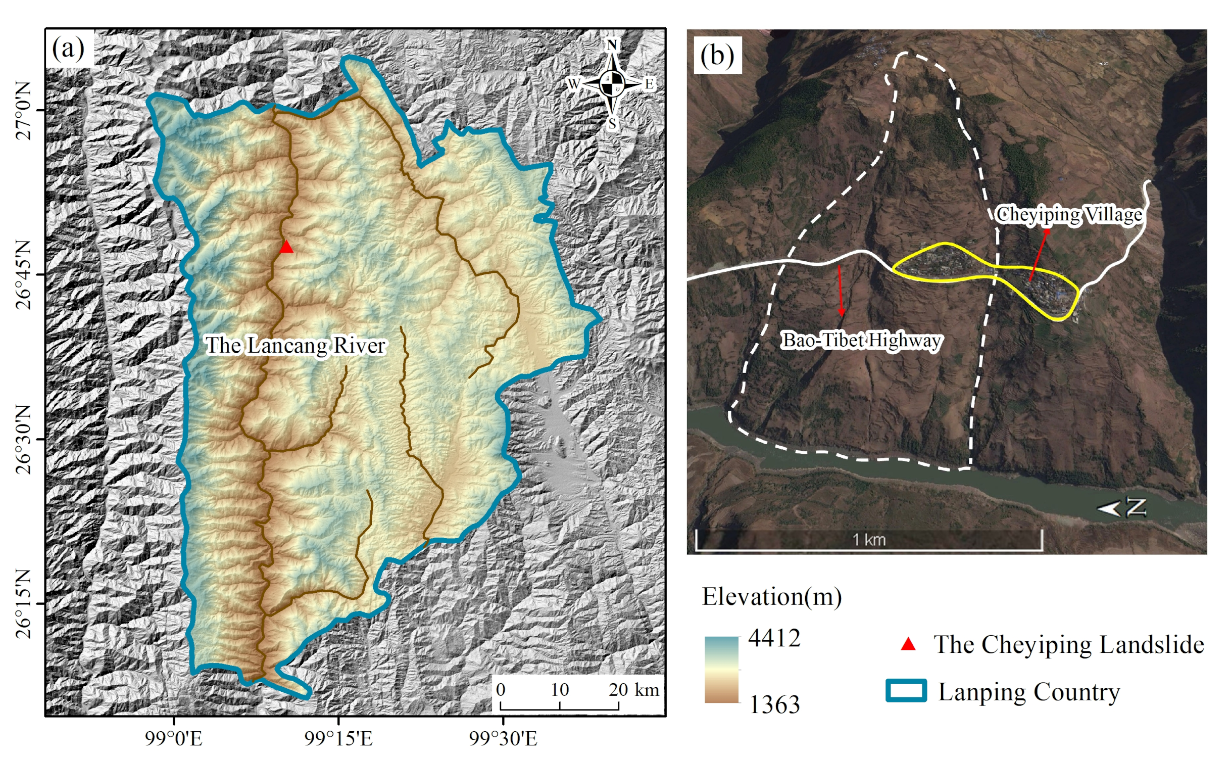
2.1. Study Area

The Cheyiping landslide is a medium-sized, slow-moving planar sliding landslide composed of clay and sand [37], which is located in Shideng Township, Lanping County, Lisu Autonomous Prefecture of Nujiang, Yunnan Province. The study area has little cultivated land, a large elevation difference, and plenty of deeply cut valleys, in which several geological disasters are distributed. Figure 1a shows the topography and geographical location of the study area. The center of landslide is located at 26.7928 N, 99.1863 E, with an altitude range of 1796 to 1855 m, a slope aspect of approximately 250 , and a terrain slope of around 25 . Located along the Lancang River, 155 households with a total of 535 people live in Cheyiping Village and the primary school on the landslide. In addition, the Bao–Tibet Highway was built in the middle of it. There have been lots of cracks appearing on the road and walls in the village because of movement in recent years. The location of the highway and the village on the landslide are shown in Figure 1b.

2.2. Data

This paper uses 60 scenes of Sentinel-1A SAR ascending data of orbit 172 acquired from 5 January 2018 to 27 December 2021. The imaging mode is IW (Interferometric Wide-swath) SLC (Single Look Complex), and the central incident angle is 39.28 . The resolution is 13.94 m in azimuth and 2.32 m in the slant range. The Sentinel-1 satellite operates in the C-band with an orbital height of about 7000 km, with a 12-day revisit period and a large-scale spatial coverage of 250 km × 250 km. It can perform all-weather and all-day high-resolution monitoring of the global land and sea surface in multi-polarization. Therefore, these characteristics of Sentinel-1A data could meet the requirements of the landslide observation. The time information of the data used is shown in Table 1.
It is necessary to remove terrain phase errors from the satellite orbit information during the process of image registration and differential interference. Therefore, the POD precise orbit data was used for orbit refinement when importing data [38,39]. The image of the study area was cropped out to improve processing efficiency (Figure 2). The SRTM1 30 m elevation data jointly measured by NASA and the Department of Defense’s National Mapping Agency (NIMA) were used in the interferometric processing to remove the topographic phase [40].

3. Methodology

The workflow of this paper is shown in Figure 3, which is mainly divided into datasets, data process, results, deformation analysis, and inducement analysis of landslide. The data processing method is described in detail here.

3.1. The Principle of PS-InSAR

The process of PS-InSAR uses multi-scene SAR images to detect highly coherent persistent scatterers (PSs) that are not affected by time and space baseline decorrelation based on a statistical analysis of the stability of amplitude and phase information in the time series. From these PSs, the topography, elevation, and atmospheric phases are estimated and eliminated before the deformation phase is ultimately separated.
Firstly, the image acquired on 16 August 2019 was selected as the super master image, and the master-slave image pairs were established to generate the connection network as shown in Figure 4a. Secondly, all the slave images are co-registered on the super master image to correct the deviation caused by the incident angle and orbit position during imaging. Next, the super master and slave images are subjected to interference processing to generate differential interferogram pair sequences, and the topographic phase is eliminated by using the DEM data. Then, the stable candidate points in the time series are selected, and the amplitude dispersion value is used to represent the phase standard deviation to measure the stability of the point target on the time series. When the coherence of the point target on the time series is smaller than a fixed value, known as the amplitude dispersion index (the ratio of SAR intensity average to Standard Deviation), it can be set as a candidate point [41]. Then, Delaunay’s triangulated irregular network was built between persistent scatterers. Linear deformation rate and elevation error are inverted in phase unwrapping. Data processing is greatly disturbed by atmospheric effects. Fortunately, the atmosphere is not correlated in time, only in space. According to this feature, the atmospheric phase could be removed through high-pass filtering in the time domain and low-pass filtering in the spatial domain on multi-view images. Therein, we can get the final average deformation rate and the deformation variable per phase, and finally convert the result of the Doppler coordinate system to the geographic coordinate system.

3.2. The Principle of SBAS-InSAR

Using a scene of the super master image, and the coherence will be weakened when the baseline becomes longer. To reduce the possibility of spatiotemporal decoherence, Berardino et al. proposed a small baseline set method that combines multiple main images to form a short spatiotemporal baseline, which ensures the coherence of the interferogram [42]. The combination of isolated data pairs with long time intervals has achieved good results for areas with fast changes in the coherence of ground objects, especially in vegetation coverage areas [43].
To begin with, the max space baseline was set as 2% of the critical baseline value, and the max time baseline was set as 90 days. The possible image connections are considered acceptable when the space and time baseline are less than the maximum thresholds. The interference pair diagram is shown in Figure 4b. Secondly, a total of 169 interferograms are generated, and the ratio of the range looks and azimuth looks is set as 4:1 in multilook processing. The Goldstein adaptive filtering method is used to remove noise, and the Delaunay MFC method is used for phase unwrapping [44,45,46,47,48,49]. The third step is orbital refinement and phase re-flattening. A Ground Control Point (GCP) file must be previously generated. Firstly, a representative image was chosen in all filtered interferograms and unwrapped images, respectively, as shown in Figure 5. Then GCPs were chosen in slant range image (Figure 5b) with reference to each phase in Figure 5a. The criteria for GCPs selection are no residual topography fringes, far away from the displacement area, and no phase jumps. Finally, 30 GCPs were selected and checked to be suitable for as many image pairs as possible. After inputting the GCP file, the phase ramp is estimated to remove the residual phase and phase ramp. Next, the deformation rate is obtained by the singular value decomposition (SVD) method, and the spatio-temporal filter is used for removing the atmospheric phase, which is the same as PS-InSAR. In the end, the displacement on the time series is calculated, and the deformation result is obtained by geocoding.

4. Results

4.1. Results in LOS Direction and Comparison

The results of the two time-series InSAR methods are shown in Figure 6a,b. It can be noted that there are few monitoring results in many places because of the decoherence. The ground objects in the research region are mostly bare soil, and natural characteristics like flora have low coherence, so there will be decoherence due to the long time baseline. The PS-InSAR and SBAS-InSAR select out high phase-correlation points for further analysis, which are mostly dispersed among man-made features, such as buildings and roads [50]. As a result, the raster is inconsistent with a few monitoring points. The red deformation result represents the deformation rate as positive, indicating that the objects move close to the satellite in the radar line-of-sight (LOS) direction, whereas the objects move away from the satellite in the LOS direction in the green area.
The average deformation rate in the study area obtained by the PS-InSAR ranges from −25.7 to 61 mm/a. However, there are insufficient monitoring points on the landslide body to establish the landslide’s deformation condition. The average deformation rate obtained by the SBAS-InSAR ranges from −15.3 to 157.8 mm/a, and the deformation magnitude of the landslide is much larger than that in other areas, which proves that this method is effective. Comparing the results of the two methods, the deformation trends of the two methods are generally consistent, but the SBAS-InSAR has far more monitoring points than PS-InSAR. The SBAS-InSAR results have more coherent points on the features with larger deformation, which depicts the deformation more accurately. These differences are mainly due to the different principles of the two methods combining the interferometric image pairs. The PS-InSAR uses only one main image to produce interference pairs, and when the time baseline between the main and auxiliary images becomes longer, the ground objects will change significantly in the natural vegetation coverage area, resulting in decoherence. Whereas the SBAS-InSAR uses the short baseline set criterion to generate image pairs, which greatly reduces the number of low-coherence points, and, thus, the results of SBAS-InSAR were selected to conduct further analysis of the Cheyiping landslide.

4.2. Projection of Deformation Direction

The deformation results obtained by time-series InSAR processing are along the radar line of sight (LOS). Deformation usually occurs in the direction of the steepest slope, so the deformation parallel to the direction of the maximum slope is regarded to indicate the deformation features of a landslide [51,52]. The projection method of deformation rate proposed by Colesanti et al. in 2006 is used to project the deformation from LOS to the maximum slope direction (slope) [53]. The spatial relationship between LOS direction and slope direction is shown in the following Figure 7, and the projection transformation formulas are as Formulas (1) and (2).
v s l o p e = 1 cos β × v L O S
cos β = ( sin α × cos φ ) × ( sin θ × cos α s ) + ( cos α × cos φ ) × ( sin θ × sin α s ) + sin φ × cos θ
Along LOS, the direction from the target to the sensor is positive, and the direction along LOS away from the sensor is negative; along the slope, the upward movement is positive, and downward movement is negative, as indicated by the red and blue plus signs in Figure 7. When the cos β is close to 0, the v s l o p e tends toward infinity. Therefore, the fixed threshold Herrera et al. proposed was used in 2013 ( cos β = ± 0.3 ) to avoid great anomalies in the absolute value during the conversion from v s l o p e to v L O S , and v s l o p e cannot be larger than 3.33 times that of v L O S . Therefore, when cos β < 0.3 , cos β = 0.3 ; when cos β > 0.3 , cos β = 0.3 [38]. The result of projecting the LOS direction result obtained by the SBAS method to the slope direction is shown in Figure 8. The positive and negative values of the deformation rate, as well as the magnitude of the value, have altered when compared to the LOS direction result in Figure 6b. It is logical that the velocity of the landslide is negative and indicates a downward movement along the slope. The dividing line of the change in slope aspect, or the location where significant deformation occurs, is the junction. Figure 8 clearly depicts the delimitation of the Cheyiping landslide (the range shown by the black solid line).

5. Analysis and Discussion

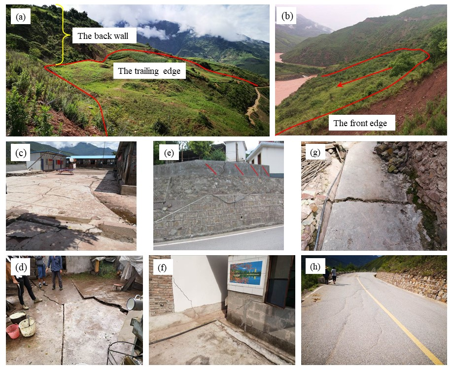
5.1. Delimitation of the Landslide

According to the slope direction results in Figure 8, the deformation rate of the landslide varies from −528.3∼−15.9 mm/a, and the plane shape of the landslide presents an irregular triangle with a length of approximately 1500 m from east to west and a width of approximately 800 m from north to south. According to the field investigation data, the landslide covers an area of about 0.8 km 2 , the thickness of the landslide body ranges from 7 to 35 m, the average thickness is about 10 m, and the volume of the landslide body is about 8 million m 3 . The front edge of the landslide is bounded by the left bank of the Lancang River, a road in the south, gullies in the north, and the rear wall of the landslide which extends to Beizhiqing Village.

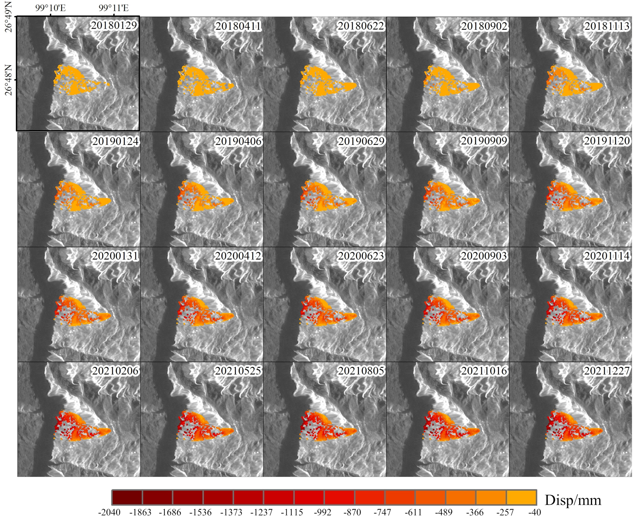
5.2. Time Series Change of Landslide Deformation Field

The regional distribution of the landslide surface deformation differs significantly. Figure 8 depicts cross-sections of the landslide body with the greatest deformation rate (as shown by the white dashed line), from which we retrieved the deformation rate and cumulative deformation in a partial time series. The deformation change of Profile A and Profile B is shown in Figure 9.
Figure 9a illustrates that the farther away from the Lancang River, the slower the landslide deforms. The sliding rate is the most extreme along the river bank, where the deformation rate surpasses −430 mm/a and the highest settlement is about 1790 mm. In Figure 9b, the landslide deformation rate increases, then decrease, and finally increases again. There are two subsidence centers on profile B located at 0.38 km and 0.8 km, and the highest subsidence rate reaches −230 mm/a, and the greatest deformation is −850 mm. It is worth noting that on the deformation curves of profiles A and B, the deformation of the middle part is smaller than that of the neighborhood. The positions of 0.57 km of profile line A and 0.6 km of profile line B are Bao–Tibet highway and Cheyiping village, and the cement floor is more stable than that of the soil. Therefore, there is an upward trend in the middle of settlement curves. Figure 10c–h shows the deformation photos. There are many cracks in the ground in the village (Figure 10c,d), on the walls of houses (Figure 10e,f), and on the roads (Figure 10g,h). In general, the landslide sinks at different rates over time. The foot of the landslide body is the most active zone of deformation, and the village and highway are relatively stable.
To further investigate the changes in landslide movement in the time dimension, we generated time series deformation of the overall landslide images presented in Figure 11. It can be seen that the deformation of the landslide developed progressively from the front edge to the trailing edge, and the sliding range on the horizontal projection surface grew. In the height direction, the magnitude of sinking is likewise increasing. It is worth noting that the front edge of the landslide along the Lancang River demonstrates deformation characteristics before the trailing edge, and the front edge drives the trailing edge to slide, demonstrating traction sliding characteristics.
Based on the deformation characteristics of various portions of the landslide, five distinct areas a, b, c, d, and e were identified. Figure 12 shows manual field survey photos and monitoring results in these areas. The field investigation reveals that the trailing edge generates cracks and subsidence (Figure 12a). The deformation rate in Area a is around −140 mm/a (as shown in Figure 12f), with a cumulative deformation of −560 mm (as shown in Figure 12g). Lateral surface cracks have developed in the top and middle parts of the landslide, spreading to the north and south sides, and the vertical dislocation is visible on both sides of the crack (Figure 12b). The typical points in Area b deform at a rate of roughly −220 mm/a, with a cumulative deformation of −880 mm. However, because the Bao-Tibet Highway runs through the heart of the landslide, and it is near the village, the stability of the landslide is critical. The field photos demonstrate that the road has begun to crack, and the fissures are growing, where noticeable subsidence and dislocation are apparent. At the same time, the ground in the village was fractured, and the cracks were repaired with mortar by the villagers (Figure 12c). The deformation rate of the characteristic points in Area c is about −170 mm/a, and the accumulated settlement reaches −680 mm. Area d is located in the middle and lower part of the landslide (Figure 12d), with more cracks on the surface than the upper part, the deformation rate is around −290 mm/a, and the accumulated settlement is −1160 mm. The front edge of the landslide lies near the Lancang River, and the deformation in Area e is the most noticeable (Figure 12e). As the landslide descends, the landslide continues to crack and sink. The deformation rate in Area e is measured at a maximum of −430 mm/a, and the accumulated subsidence is −1790 mm, so the front edge is vulnerable to slide and collapse.

5.3. Seasonal Movement Characteristics of Landslides

Figure 12g shows the cumulative deformation of the feature points over time, which is tentatively judged to be brought about by seasonal rainfall, given the physical setting of the study area. Specifically, the landslide deformation rate is significantly accelerated in the rainy season and slowed down in the wet season. The study area has distinct dry and wet seasons, with rainfall concentrated from May to October. According to different motion change characteristics, we plotted the cumulative deformation for selected points in areas a and b (as shown in Figure 12g) in Figure 13a and areas c, d, and e in Figure 13b. Figure 13 shows the relationship between the total deformation and the monthly average rainfall.
It can be seen from Figure 13 that the rainfall mainly takes place from May to October, and precipitation always reaches its peak in July, with the maximum average total rainfall in July 2019 reaching 462 mm. These rainfall season months are marked as mauve blocks, and the rest are wet season months. Time series analysis reveals that the displacement is corrected to the precipitation, and the rainfall variations have more impact on the middle and lower part of the landslide body than on the top body. The cumulative deformation curves of areas a and b have a slight trend of accelerated deformation after every wet season, as shown by the periods of time in the black dashed lines and red arrows in Figure 13a. The cumulative deformation curves of areas c, d, and e show segmented changes, and there are four acceleration periods in Figure 13b. Around four rainy seasons (from July 2018 to January 2019, from July 2019 to February 2020, from August 2020 to February 2021, and from September 2021 to November 2021), the slope of the curves increased, indicating the deformation accelerated, and the curves flattened in the rest months (from February 2019 to June 2019, from March 2020 to July 2020 and from March 2021 to August 2021). The landslide has clearly changed during the last four years. The cumulative deformation of Area a, which is the slowest, grew by four times from 100 mm to 500 mm. Area e had the most dramatic deformation, reaching 1700 mm by the end of 2021, more than three times that of 2018.
Analyzing and comparing the change characteristics of the deformation variable curves in these five regions, it was found that the slope of the curve becomes steeper one to two months after the first rainy month. For example, in Figure 13b, the rainy seasons started in May from 2018 to 2021, whereas the acceleration period began in July 2018, June 2019, August 2020, and August 2021 separately. Moreover, the influence of the precipitation on the landslide body often lasts for several months, as evidenced by the fact that the accelerated deformation ended in January 2019, February 2020, February 2021, and November 2021. Therefore, seasonal rainfall has a strong inducing effect on landslide deformation. The generation and disappearance of this aggravating effect will not be reflected immediately, but are usually delayed for a period of time, which has been found in many studies [54,55]. This is because it takes a period of time for rainfall to infiltrate into the landslide rock mass, so its influence on the deformation rate of the landslide has a hysteresis, which is consistent with many studies [56,57,58,59].

5.4. The Inducement of the Landslide

Whether the landslide slips or not depends on the relationship between the slope angle and the critical angle, and the critical angle is influenced by the block material composition, size, shape, and water content. Most of the non-earthquake landslides are triggered by broken structures, soil strength, intensive rainfall, and the effect of water level in many studies [60,61,62]. Accordingly, the causes of the Cheyiping landslide are divided into internal causes, mainly topography, geology, geotechnical properties, and external causes of water for analysis.

5.4.1. Topography and Geology

The Cheyiping landslide is located in an area of the sloping terrain, with an overall the slope direction of about 255 , a slope length of 1500 m, a terrain slope of 15 to 20 , a village side slope height of 1.5 to 4.7 m, and a slope gradient of 65 to 280 . Morphologically, it is a moderately steep and long slope, which can be classified as a loose cap rock slope according to the slope process. With the sliding of the slope body concentrated on the front edge and the middle, the movement rate of the back end is small and belongs to a traction landslide. The topography of the area has a steep slope and a large relative height difference. resulting in a large gravitational potential energy of soil on the slope, which provides the impetus for the sliding of the slope material [60]. According to regional geological data, the Cheyiping fault developed on the west side of the Bao-Tibet highway at about 350–400 m, which could cause the geological structure to fragment and change the tectonic stress field, thus, increasing the risk of landslides [56].

5.4.2. Lithology

In Lanping county, the Mesozoic strata are mainly exposed, followed by the Cenozoic and Paleozoic, and a very small amount of unidentified metamorphic rock series. The Mesozoic is almost all over the region, mainly composed of Cretaceous, Jurassic, Triassic siltstone, silty mudstone, and quartz sandstone. The Cenozoic is the sandstone, conglomerate, and calcareous siltstone of the Tertiary, and the sandy clay and sandy gravel of the Quaternary. Paleozoic strata are dominated by mudstones, sandstones, and Carboniferous bioclastic tuffs, schists, and andesites. The geology of the study area is shown in Figure 14 (source of data: https://geocloud.cgs.gov.cn, accessed on 27 September 2022). Meanwhile, there are small amounts of basalt, andesite, and other volcanic rocks located in the eastern and western margins. The rock mass is mainly composed of layered and fractured structural soft rocks, so the weak structure affects the engineering geological properties [63].
The surface of the landslide is brownish-red and brownish-yellow clay with debris in the residual slope of the Quaternary System. The soil structure is loose, the water permeability is strong, the soil softens and collapses when it meets water, and the stability is poor; thus, excavation disturbance is prone to collapse and landslide. The underlying stratum is the purple-red and grey-green sandstone and mudstone weathering rock of the Jurassic Middle Jurassic Huakai Zuo Group (J2h), which is mainly exposed on the ridges of the north and south sides of the village and on the steeper topography of the village, with weak lithology. The rocks within the slope are strongly weathered mudstone interspersed with muddy siltstone, which is a weak structural plane due to the poor connectivity in rock and soil bodies. The dip Angle of the structural plane is similar to that of the natural slope, which forms the sliding plane.

5.4.3. Influence of Seasonal Rainfall and Water Level

Water is a major cause of landslides [61]. The involvement of water removes the adsorption bond between soil particles, changes the pore water pressure, reduces the resistance to sliding, and erodes the strength of the soil. According to previous studies [64,65], continuous rainfall and rapid changes in the water level have a joint impact on the displacement rate of the landslide. The stability of the landslide decreased with the increase in rainfall intensity and the changes in the water level of the Lancang River. The combination of these two factors in the study area may be the main reason for the accelerated deformation of the Cheyiping landslide. Moreover, the unregulated discharge of water for domestic use by residents in the village and the erosion of the two gullies on the slope impair the stability of the slope.
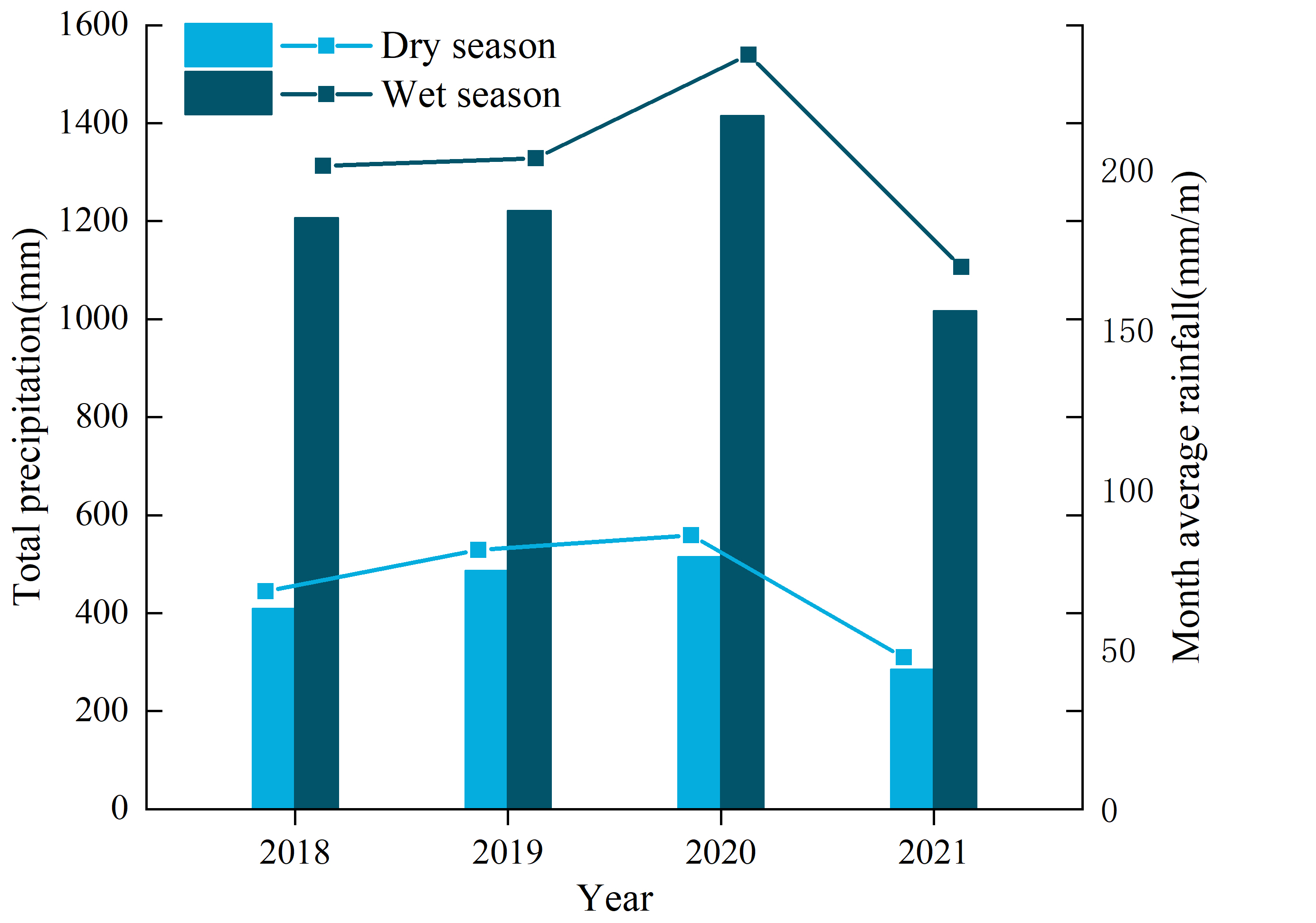
  • Seasonal rainfall. The region of the landslide is characterized by the low-latitude mountain monsoon and typical vertical distribution of the three-dimensional climate, with the highest temperature in July and the lowest temperature in January. With a clear division between wet and dry seasons, the rainfall in the study area is regular. The average annual precipitation is 1002.4 mm and the average annual rainfall is 158 days, with the rainy season from late May to mid-October, which accounts for over 90% of the annual precipitation. The monsoonal climate and seasonal precipitation concentrated in the summer provide a strong trigger for the landslide. According to the ERA5-Land reanalysis dataset, the seasonal precipitation around the Cheyiping area from 2018 to 2021 is shown in Figure 15, indicating that the amount of rainfall in the rainy season is much greater than in the wet season.
    Persistent rainfall increases the pore pressure of the landslide, which reduces the sheer strength of the soil, the bond between the rock particles, and the friction within the landslide, resulting in a high risk of landslides [66]. Water causes expansion and contraction of geotechnical particles, which can alter the pore pressure of the landslide and seasonal rainfall makes this change frequently, whereas pore pressure changes are the main driver of landslide movement, and the larger pore pressure changes can induce landslides [67].
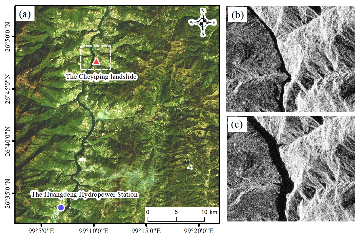
  • Erosion and water level rise of the Lancang River. The study area is located in the high mountain area and canyon in the middle-upper reaches of the Lancang River. The Lancang River runs north to south through the mountain valley in Lanping County, with a natural drop of 127 m, an average slope of 9.8%, an average annual flow of 909 m 3 , and the driest flow of 277 m 3 . Moreover, the front edge of the Cheyiping landslide is adjacent to the Lancang River. The Huangdeng Hydropower Station is built at the position of 99.1197 E, 26.5597 N, which is 26 km away from the landslide, as shown in Figure 16a. The normal storage level of the reservoir is 1619 m, which started to store water in May 2018. The water level in the Cheyiping landslide section was 1557 m; however, after the impoundment, the water level rose by 62 m. By checking the width of the river surface in the radar image Figure 16b,c, it is possible to determine that the water level has significantly risen from January 2018 to January 2019.
    Changes in water level have multiple effects on the stability of landslides. The rise in water level caused by the Huangdeng Hydropower Station storage will affect the geotechnical strength of the slope, the groundwater level, and the pressure difference between the water inside and outside the slope. When the water level changes, there is a lag in the change of the groundwater level, and the pressure difference between the inside and outside of the landslide will disrupt the original equilibrium of the slope [68]. When the water level rises, the external pressure enhances the stability of the slope to a certain extent, and in this case, the accelerated deformation of the slope is typically a result of the softening impact of the water. Therefore, the deformation rate of the slope during the high water level is significantly higher than during the low water level [69].

6. Conclusions

In this study, Sentinel-1A images were collected, and the time-series deformation monitoring results of the Cheyiping landslide from 5 January 2018 to 27 December 2021 were obtained using the time-series InSAR technology. The monitoring results of the PS-InSAR and the SBAS-InSAR show the same deformation trend in most regions, while the SBAS-InSAR intensively detects the landslide with many more monitoring points. The results of the slope direction shows that the deformation rate of the landslide increases from the back edge to the front edge, the deformation rate at the foot of the slope near the Lancang River reaches approximately −430 mm/a, and the accumulated subsidence during the study period is as high as −1790 mm. The front edge of the landslide occurs first, driving the overall movement of the landslide. Based on these results, it was found that the intense concentrated seasonal rainfall accelerates the surface deformation of the slope, and the deformation velocity slows down in the dry season, meaning the landslide movement shows a periodical accelerated trend. Moreover, the water level change of the Lancang River brought by the water storage of the Huangdeng hydropower station downstream makes the landslide destabilized, and seasonal rainfall and water level changes of the Lancang River were the primary causes for the significant movement of the Cheyiping landslide.
In summary, the time-series InSAR technology is feasible for monitoring the deformation of the Cheyiping landslide. The analysis of the time-series changes of landslide deformation based on geological and geomorphological factors, seasonal rainfall, and water level changes of the Lancang River can predict the landslide movement. In the future, accurate landslide hazard warnings could be carried out by combining field survey data with remote sensing data, thus, providing protection for the life and property safety of the residents in this area.

Author Contributions

Conceptualization, L.Z. and Y.C.; methodology, L.Z., Y.C. and Y.G.; software, Y.G. and J.L.; validation, H.Z. and X.L.; formal analysis, Y.G.; investigation, Y.G. and H.Z.; writing—original draft preparation, Y.G.; writing—review and editing, L.Z.; visualization, Y.G. and Q.Z.; supervision, L.Z.; project administration, L.Z.; funding acquisition, L.Z. All authors have read and agreed to the published version of the manuscript.

Funding

This work was supported by the Joint Funds of the National Natural Science Foundation of China [grant number U2268217], the National Natural Science Foundation of China [grant number 41876226], and the Strategic Priority Research Program of the Chinese Academy of Sciences [grant numbers XDA19090135]. L. Zhang is the corresponding author of this paper (zhanglu@radi.ac.cn).

Data Availability Statement

The Sentinel-1A data is available on ASF Data Search (https://search.asf.alaska.edu), the SRTM (The Shuttle Radar Topography Mission) elevation data are available online at http://srtm.csi.cgiar.org/, precipitation data is provided by ERA5-Land reanalysis dataset (https://cds.climate.copernicus.eu), and the geological map are based on data from GeoCloud (https://geocloud.cgs.gov.cn). All links accessed on 27 September 2022.

Acknowledgments

The author would like to thank the editors and the reviewers for their suggestions and comments, which helped us improve the study greatly.

Conflicts of Interest

The authors declare no conflict of interest.

References

  1. Cruden, D.M. A simple definition of a landslide. Bull. Int. Assoc. Eng. Geol. 1991, 43, 27–29. [Google Scholar] [CrossRef]
  2. Dai, F.; Lee, C.; Ngai, Y. Landslide risk assessment and management: An overview. Eng. Geol. 2002, 64, 65–87. [Google Scholar] [CrossRef]
  3. Froude, M.J.; Petley, D.N. Global fatal landslide occurrence from 2004 to 2016. Nat. Hazards Earth Syst. Sci. 2018, 18, 2161–2181. [Google Scholar] [CrossRef] [Green Version]
  4. Turner, A.G.; Annamalai, H. Climate change and the South Asian summer monsoon. Nat. Clim. Chang. 2012, 2, 587–595. [Google Scholar] [CrossRef]
  5. Petley, D. Global patterns of loss of life from landslides. Geology 2012, 40, 927–930. [Google Scholar] [CrossRef]
  6. Kirschbaum, D.; Adler, R.; Adler, D.; Peters-Lidard, C.; Huffman, G. Global Distribution of Extreme Precipitation and High-Impact Landslides in 2010 Relative to Previous Years. J. Hydrometeorol. 2012, 13, 1536–1551. [Google Scholar] [CrossRef] [Green Version]
  7. Huang, R. Large-Scale Landslides and Their Sliding Mechanisms in China Since the 20th Century. Chin. J. Rock Mech. Eng. 2007, 26, 433–454. [Google Scholar]
  8. Runqiu, H. Some catastrophic landslides since the twentieth century in the southwest of China. Landslides 2009, 6, 69–81. [Google Scholar] [CrossRef]
  9. Lin, Q.; Wang, Y. Spatial and temporal analysis of a fatal landslide inventory in China from 1950 to 2016. Landslides 2018, 15, 2357–2372. [Google Scholar] [CrossRef]
  10. Iverson, R.M.; George, D.L.; Allstadt, K.; Reid, M.E.; Collins, B.D.; Vallance, J.W.; Schilling, S.P.; Godt, J.W.; Cannon, C.M.; Magirl, C.S.; et al. Landslide mobility and hazards: Implications of the 2014 Oso disaster. Earth Planet. Sci. Lett. 2015, 412, 197–208. [Google Scholar] [CrossRef] [Green Version]
  11. Collins, B.D.; Reid, M.E. Enhanced landslide mobility by basal liquefaction: The 2014 State Route 530 (Oso), Washington, landslide. Geol. Soc. Am. Bull. 2020, 132, 451–476. [Google Scholar] [CrossRef]
  12. Ma, S.; Xu, C.; Xu, X.; He, X.; Qian, H.; Jiao, Q.; Gao, W.; Yang, H.; Cui, Y.; Zhang, P.; et al. Characteristics and causes of the landslide on July 23, 2019 in Shuicheng, Guizhou Province, China. Landslides 2020, 17, 1441–1452. [Google Scholar] [CrossRef]
  13. Zhao, W.; Wang, R.; Liu, X.; Ju, N.; Xie, M. Field survey of a catastrophic high-speed long-runout landslide in Jichang Town, Shuicheng County, Guizhou, China, on July 23, 2019. Landslides 2020, 17, 1415–1427. [Google Scholar] [CrossRef]
  14. Tofani, V.; Raspini, F.; Catani, F.; Casagli, N. Persistent Scatterer Interferometry (PSI) Technique for Landslide Characterization and Monitoring. Remote Sens. 2013, 5, 1045–1065. [Google Scholar] [CrossRef] [Green Version]
  15. Gili, J.; Corominas, J.; Rius, J. Using Global Positioning System techniques in landslide monitoring. Eng. Geol. 2000, 55, 167–192. [Google Scholar] [CrossRef]
  16. Yin, Y.; Wang, H.; Gao, Y.; Li, X. Real-time monitoring and early warning of landslides at relocated Wushan Town, the Three Gorges Reservoir, China. Landslides 2010, 7, 339–349. [Google Scholar] [CrossRef]
  17. Mora, P.; Baldi, P.; Casula, G.; Fabris, M.; Ghirotti, M.; Mazzini, E.; Pesci, A. Global Positioning Systems and digital photogrammetry for the monitoring of mass movements: Application to the Ca’ di Malta landslide (northern Apennines, Italy). Eng. Geol. 2003, 68, 103–121. [Google Scholar] [CrossRef]
  18. Shi, X.; Xu, Q.; Zhang, L.; Zhao, K.; Dong, J.; Jiang, H.; Liao, M. Surface displacements of the Heifangtai terrace in Northwest China measured by X and C-band InSAR observations. Eng. Geol. 2019, 259, 105181. [Google Scholar] [CrossRef]
  19. Sun, Y.J.; Zhang, D.; Shi, B.; Tong, H.J.; Wei, G.Q.; Wang, X. Distributed acquisition, characterization and process analysis of multi-field information in slopes. Eng. Geol. 2014, 182, 49–62. [Google Scholar] [CrossRef]
  20. Dong, J.; Zhang, L.; Li, M.; Yu, Y.; Liao, M.; Gong, J.; Luo, H. Measuring precursory movements of the recent Xinmo landslide in Mao County, China with Sentinel-1-and ALOS-2 PALSAR-2 datasets. Landslides 2018, 15, 135–144. [Google Scholar] [CrossRef]
  21. Colesanti, C.; Wasowski, J. Investigating landslides with space-borne synthetic aperture radar (SAR) interferometry. Eng. Geol. 2006, 88, 173–199. [Google Scholar] [CrossRef]
  22. Xiao, B.; Zhao, J.; Li, D.; Zhao, Z.; Xi, W.; Zhou, D. The Monitoring and Analysis of Land Subsidence in Kunming (China) Supported by Time Series InSAR. Sustainability 2022, 14, 12387. [Google Scholar] [CrossRef]
  23. Gabriel, A.K.; Goldstein, R.M.; Zebker, H.A. Method for Detecting Surface Motions and Mapping Small Terrestrial or Planetary Surface Deformations with Synthetic Aperture Radar. U.S. Patent US4975704A, 4 December 1990. [Google Scholar]
  24. Gabriel, A.; Goldstein, R.; Zebker, H. Mapping Small Elevation Changes over Large Areas—Differential Radar Interferometry. J. Geophys.-Res.-Solid Earth Planets 1989, 94, 9183–9191. [Google Scholar] [CrossRef]
  25. Amelung, F.; Galloway, D.; Bell, J.; Zebker, H.; Laczniak, R. Sensing the ups and downs of Las Vegas: InSAR reveals structural control of land subsidence and aquifer-system deformation. Geology 1999, 27, 483–486. [Google Scholar] [CrossRef]
  26. Massonnet, D.; Rossi, M.; Carmona, C.; Adragna, F.; Peltzer, G.; Feigl, K.; Rabaute, T. The Displacement Field of the Landers Earthquake Mapped by Radar Interferometry. Nature 1993, 364, 138–142. [Google Scholar] [CrossRef]
  27. Kenyi, L.; Kaufmann, V. Estimation of rock glacier surface deformation using SAR interferometry data. IEEE Trans. Geosci. Remote Sens. 2003, 41, 1512–1515. [Google Scholar] [CrossRef]
  28. Kimura, H.; Yamaguchi, Y. Detection of landslide areas using satellite radar interferometry. Photogramm. Eng. Remote Sens. 2000, 66, 337–344. [Google Scholar]
  29. Liu, G.; Buckley, S.M.; Ding, X.; Chen, Q.; Luo, X. Estimating Spatiotemporal Ground Deformation With Improved Permanent-Scatterer Radar Interferometry. IEEE Trans. Geosci. Remote Sens. 2009, 47, 2762–2772. [Google Scholar] [CrossRef]
  30. Wasowski, J.; Bovenga, F. Investigating landslides and unstable slopes with satellite Multi Temporal Interferometry: Current issues and future perspectives. Eng. Geol. 2014, 174, 103–138. [Google Scholar] [CrossRef]
  31. Colesanti, C.; Ferretti, A.; Prati, C.; Rocca, F. Monitoring landslides and tectonic motions with the Permanent Scatterers Technique. Eng. Geol. 2003, 68, 3–14. [Google Scholar] [CrossRef]
  32. Ferretti, A.; Prati, C.; Rocca, F. Nonlinear subsidence rate estimation using permanent scatterers in differential SAR interferometry. IEEE Trans. Geosci. Remote Sens. 2000, 38, 2202–2212. [Google Scholar] [CrossRef] [Green Version]
  33. Berardino, P.; Fornaro, G.; Lanari, R.; Sansosti, E. A new algorithm for surface deformation monitoring based on small baseline differential SAR interferograms. IEEE Trans. Geosci. Remote Sens. 2002, 40, 2375–2383. [Google Scholar] [CrossRef]
  34. Osmanoglu, B.; Sunar, F.; Wdowinski, S.; Cabral-Cano, E. Time series analysis of InSAR data: Methods and trends. ISPRS J. Photogramm. Remote Sens. 2016, 115, 90–102. [Google Scholar] [CrossRef]
  35. Zhao, C.; Kang, Y.; Zhang, Q.; Lu, Z.; Li, B. Landslide Identification and Monitoring along the Jinsha River Catchment (Wudongde Reservoir Area), China, Using the InSAR Method. Remote Sens. 2018, 10, 993. [Google Scholar] [CrossRef] [Green Version]
  36. Lacroix, P.; Handwerger, A.L.; Bievre, G. Life and death of slow-moving landslides. Nat. Rev. Earth Environ. 2020, 1, 404–419. [Google Scholar] [CrossRef]
  37. Hungr, O.; Leroueil, S.; Picarelli, L. The Varnes classification of landslide types, an update. Landslides 2014, 11, 167–194. [Google Scholar] [CrossRef]
  38. Herrera, G.; Gutierrez, F.; Garcia-Davalillo, J.C.; Guerrero, J.; Notti, D.; Galve, J.P.; Fernandez-Merodo, J.A.; Cooksley, G. Multi-sensor advanced DInSAR monitoring of very slow landslides: The Tena Valley case study (Central Spanish Pyrenees). Remote Sens. Environ. 2013, 128, 31–43. [Google Scholar] [CrossRef]
  39. Cigna, F.; Bateson, L.B.; Jordan, C.J.; Dashwood, C. Simulating SAR geometric distortions and predicting Persistent Scatterer densities for ERS-1/2 and ENVISAT C-band SAR and InSAR applications: Nationwide feasibility assessment to monitor the landmass of Great Britain with SAR imagery. Remote Sens. Environ. 2014, 152, 441–466. [Google Scholar] [CrossRef] [Green Version]
  40. Feng, W.; Jiawei, D.; Xiaoyu, Y.I.; Zhang, G. Deformation Analysis of Woda Village Old Landslide in Jinsha River Basin Using Sbas-Insar Technology. J. Eng. Geol. 2020, 28, 384–393. [Google Scholar]
  41. Ferretti, A.; Prati, C.; Rocca, F. Permanent scatterers in SAR interferometry. IEEE Trans. Geosci. Remote Sens. 2001, 39, 8–20. [Google Scholar] [CrossRef]
  42. Lanari, R.; Lundgren, P.; Manzo, M.; Casu, F. Satellite radar interferometry time series analysis of surface deformation for Los Angeles, California. Geophys. Res. Lett. 2004, 31, 021294. [Google Scholar] [CrossRef]
  43. Lanari, R.; Casu, F.; Manzo, M.; Zeni, G.; Berardino, P.; Manunta, M.; Pepe, A. An overview of the small BAseline subset algorithm: A DInSAR technique for surface deformation analysis. Pure Appl. Geophys. 2007, 164, 637–661. [Google Scholar] [CrossRef]
  44. Tang, H.; Wasowski, J.; Juang, C.H. Geohazards in the three Gorges Reservoir Area, China Lessons learned from decades of research. Eng. Geol. 2019, 261, 105267. [Google Scholar] [CrossRef]
  45. Jia, H.; Wang, Y.; Ge, D.; Deng, Y.; Wang, R. InSAR Study of Landslides: Early Detection, Three-Dimensional, and Long-Term Surface Displacement Estimation-A Case of Xiaojiang River Basin, China. Remote Sens. 2022, 14, 1759. [Google Scholar] [CrossRef]
  46. Yao, J.; Yao, X.; Liu, X. Landslide Detection and Mapping Based on SBAS-InSAR and PS-InSAR: A Case Study in Gongjue County, Tibet, China. Remote. Sens. 2022, 14, 4728. [Google Scholar] [CrossRef]
  47. Soltanieh, A.; Macciotta, R. Updated Understanding of the Ripley Landslide Kinematics Using Satellite InSAR. Geosciences 2022, 12, 298. [Google Scholar] [CrossRef]
  48. Jiao, R.; Wang, S.; Yang, H.; Guo, X.; Han, J.; Pei, X.; Yan, C. Comprehensive Remote Sensing Technology for Monitoring Landslide Hazards and Disaster Chain in the Xishan Mining Area of Beijing. Remote Sens. 2022, 14, 4695. [Google Scholar] [CrossRef]
  49. Mishra, V.; Jain, K. Satellite based assessment of artificial reservoir induced landslides in data scarce environment: A case study of Baglihar reservoir in India. J. Appl. Geophys. 2022, 205, 104754. [Google Scholar] [CrossRef]
  50. Perissin, D.; Ferretti, A. Urban-target recognition by means of repeated spaceborne SAR images. IEEE Trans. Geosci. Remote Sens. 2007, 45, 4043–4058. [Google Scholar] [CrossRef]
  51. Bejar-Pizarro, M.; Notti, D.; Mateos, R.M.; Ezquerro, P.; Centolanza, G.; Herrera, G.; Bru, G.; Sanabria, M.; Solari, L.; Duro, J.; et al. Mapping Vulnerable Urban Areas Affected by Slow-Moving Landslides Using Sentinel-1 InSAR Data. Remote Sens. 2017, 9, 876. [Google Scholar] [CrossRef] [Green Version]
  52. Aslan, G.; Foumelis, M.; Raucoules, D.; De Michele, M.; Bernardie, S.; Cakir, Z. Landslide Mapping and Monitoring Using Persistent Scatterer Interferometry (PSI) Technique in the French Alps. Remote Sens. 2020, 12, 1305. [Google Scholar] [CrossRef] [Green Version]
  53. Cascini, L.; Fornaro, G.; Peduto, D. Advanced low- and full-resolution DInSAR map generation for slow-moving landslide analysis at different scales. Eng. Geol. 2010, 112, 29–42. [Google Scholar] [CrossRef]
  54. Handwerger, A.L.; Huang, M.H.; Fielding, E.J.; Booth, A.M.; Burgmann, R. A shift from drought to extreme rainfall drives a stable landslide to catastrophic failure. Sci. Rep. 2019, 9, 1569. [Google Scholar] [CrossRef] [PubMed]
  55. Dille, A.; Kervyn, F.; Handwerger, A.L.; d’Oreye, N.; Derauw, D.; Bibentyo, T.M.; Samsonov, S.; Malet, J.P.; Kervyn, M.; Dewitte, O. When image correlation is needed: Unravelling the complex dynamics of a slow-moving landslide in the tropics with dense radar and optical time series. Remote Sens. Environ. 2021, 258, 112402. [Google Scholar] [CrossRef]
  56. Wang, Y.; Cui, X.; Che, Y.; Li, P.; Jiang, Y.; Peng, X. Automatic Identification of Slope Active Deformation Areas in the Zhouqu Region of China With DS-InSAR Results. Front. Environ. Sci. 2022, 10, 883427. [Google Scholar] [CrossRef]
  57. Ma, S.; Qiu, H.; Hu, S.; Yang, D.; Liu, Z. Characteristics and geomorphology change detection analysis of the Jiangdingya landslide on July 12, 2018, China. Landslides 2021, 18, 383–396. [Google Scholar] [CrossRef]
  58. Fobert, M.A.; Singhroy, V.; Spray, J.G. InSAR Monitoring of Landslide Activity in Dominica. Remote Sens. 2021, 13, 815. [Google Scholar] [CrossRef]
  59. Xue, C.; Chen, K.; Tang, H.; Liu, P. Heavy rainfall drives slow-moving landslide in Mazhe Village, Enshi to a catastrophic collapse on 21 July 2020. Landslides 2022, 19, 177–186. [Google Scholar] [CrossRef]
  60. Zhu, Y.; Yao, X.; Yao, L.; Zhou, Z.; Ren, K.; Li, L.; Yao, C.; Gu, Z. Identifying the Mechanism of Toppling Deformation by InSAR: A Case Study in Xiluodu Reservoir, Jinsha River. Landslides 2022, 19, 2311–2327. [Google Scholar] [CrossRef]
  61. Medhat, N.I.; Yamamoto, M.y.; Tolomei, C.; Harbi, A.; Maouche, S. Multi-temporal InSAR analysis to monitor landslides using the small baseline subset (SBAS) approach in the Mila Basin, Algeria. Terra Nova 2022, 34, 407–423. [Google Scholar] [CrossRef]
  62. Liu, Y.; Yang, H.; Wang, S.; Xu, L.; Peng, J. Monitoring and Stability Analysis of the Deformation in the Woda Landslide Area in Tibet, China by the DS-InSAR Method. Remote Sens. 2022, 14, 532. [Google Scholar] [CrossRef]
  63. Ying-Wen, Y.; Wei, L.; Na, F. The Feature and Prevent-Control Policy of Geological Disaster of Lanping in Nujiang, Yunnan. Yunnan Geol. 2019, 38, 2019. [Google Scholar]
  64. Li, D.; Yin, K.; Leo, C. Analysis of Baishuihe landslide influenced by the effects of reservoir water and rainfall. Environ. Earth Sci. 2010, 60, 677–687. [Google Scholar] [CrossRef]
  65. Xia, M.; Ren, G.M.; Ma, X.L. Deformation and mechanism of landslide influenced by the effects of reservoir water and rainfall, Three Gorges, China. Nat. Hazards 2013, 68, 467–482. [Google Scholar] [CrossRef]
  66. Handwerger, A.L.; Fielding, E.J.; Huang, M.H.; Bennett, G.L.; Liang, C.; Schulz, W.H. Widespread Initiation, Reactivation, and Acceleration of Landslides in the Northern California Coast Ranges due to Extreme Rainfall. J. Geophys.-Res.-Earth Surf. 2019, 124, 1782–1797. [Google Scholar] [CrossRef] [Green Version]
  67. Schulz, W.H.; McKenna, J.P.; Kibler, J.D.; Biavati, G. Relations between hydrology and velocity of a continuously moving landslide-evidence of pore-pressure feedback regulating landslide motion? Landslides 2009, 6, 181–190. [Google Scholar] [CrossRef]
  68. Zhao, S.; Zeng, R.; Zhang, H.; Meng, X.; Zhang, Z.; Meng, X.; Wang, H.; Zhang, Y.; Liu, J. Impact of Water Level Fluctuations on Landslide Deformation at Longyangxia Reservoir, Qinghai Province, China. Remote Sens. 2022, 14, 212. [Google Scholar] [CrossRef]
  69. Chen, M.l.; Qi, S.c.; Lv, P.f.; Yang, X.g.; Zhou, J.w. Hydraulic response and stability of a reservoir slope with landslide potential under the combined effect of rainfall and water level fluctuation. Environ. Earth Sci. 2021, 80, 25. [Google Scholar] [CrossRef]
Figure 1. Overview of the study area. (a) The geographical location of the Cheyiping landslide (the red triangle). (b) The Google map of the Cheyiping landslide, labeled with Bao–Tibet highway, Cheyiping village, and the boundary of the Cheyiping landslide.
Remotesensing 15 00051 g001
Figure 2. The Sentinel-1A SAR data coverage.
Remotesensing 15 00051 g002
Figure 3. The workflow of the study.
Remotesensing 15 00051 g003
Figure 4. (a) Time−Position map of PS-InSAR. (b) Time−Position map of SBAS-InSAR. The master image is presented as a red star, the slave images are presented as black dots, and all images are marked with the serial number in Table 1. Each line represents a master-slave image pair, and the horizontal and vertical coordinates show their time and space baselines.
Remotesensing 15 00051 g004
Figure 5. (a) Filtered interferogram, which is used for determining terrain and deformation areas. (b) Unwrapped interferogram with 30 GCPs. The red plus sign represents GCPs.
Remotesensing 15 00051 g005
Figure 6. Monitoring results in LOS direction by PS-InSAR (a) and SBAS-InSAR (b), respectively. The annual average velocity results overlay the Sentinel-2 satellite data. The red raster shows uplifted deformation in the LOS direction, the green indicates descend.
Remotesensing 15 00051 g006
Figure 7. Spatial relationship between v s l o p e and v L O S directions for a point (black dot) located on the slope. v s l o p e is the deformation rate along the slope, v L O S is the deformation rate along the LOS direction. β is the angle between the v L O S and v s l o p e directions, rotating from v s l o p e to LOS direction. α is the aspect angle. φ is the slope angle. θ is the angle between the vertical direction and LOS, i.e., the incidence angle with reference to flat land. α s is the angle between the satellite azimuth and the true north direction, rotating from the north to ascending orbit direction in our study, and for the Sentinel-1A at orbit 172 is −12.
Remotesensing 15 00051 g007
Figure 8. Deformation rate and interpretation boundary of the Cheyiping landslide. Two white dotted lines represent the lines of profiles, which are labeled with start and end coordinates.
Remotesensing 15 00051 g008
Figure 9. Time−series cumulative deformation of profiles. (a) Profile A. (b) Profile B. The solid lines represent cumulative deformation from 5 January 2018, until the date, corresponding to the left vertical axis; and the dotted lines represent the average annual deformation rate of points on the profile lines, corresponding to the right vertical axis. The grey parts represent the elevation of the profiles.
Remotesensing 15 00051 g009
Figure 10. Field survey photos. (a) The trailing edge has sunk. (b) The front edge has slid. (c) Cracks in the Cheyiping primary school. (d) Cracks in villagers’ homes. (e) Fissures in the walls. (f) Cracks in houses. (g) Cracks in the road in the village. (h) Deformation of Bao–Tibet highway.
Remotesensing 15 00051 g010
Figure 11. Time−series cumulative deformation calculated from 5 January 2018 of the landslide on each acquisition date. The base map is the SAR intensity average image, and the dates are labeled on the top right corner of every subgraph.
Remotesensing 15 00051 g011
Figure 12. Field survey photos and monitoring results. (a) Cracks on the trailing edge (Area a in (f)). (b) Faults in the middle−upper part (Area b in (f)). (c) Fissures on the pavement in Cheyiping village (Area c in (f)). (d) Cracks in the middle and lower part (Area d in (f)). (e) Collapse on the front edge (Area e in (f)). (f) Deformation rates of regional typical points. (g) Accumulated settlement of three typical points in each area of (f).
Remotesensing 15 00051 g012
Figure 13. Time−series cumulative deformation of feature points. (a) The feature points in Area a, b (as shown in Figure 12f). (b) The feature points in Area c, d, e (as shown in Figure 12f).
Remotesensing 15 00051 g013
Figure 14. The geological map of the study area.
Remotesensing 15 00051 g014
Figure 15. Seasonal precipitation. Wet season: from May to October. Dry season: from January to April, November, and December.
Remotesensing 15 00051 g015
Figure 16. Variation of the Lancang River water level before and after impoundment. (a) The relative locations of the Cheyiping landslide and the Huangdeng Hydropower Station. (b) SAR image of white dotted line range in (a) on 5 January 2018. (c) SAR image of white dotted line range in (a) on 24 January 2019.
Remotesensing 15 00051 g016
Table 1. Acquisition time of SAR data.
NumberDateNumberDateNumberDateNumberDate
15 January 20181631 December 2018317 January 20204613 January 2021
229 January 20181724 January 20193231 January 2020476 February 2021
322 February 20181817 February 20193324 February 20204814 March 2021
418 March 20181913 March 20193419 March 2020497 April 2021
511 April 2018206 April 20193512 April 2020501 May 2021
65 May 20182112 May 2019366 May 20205125 May 2021
729 May 2018225 June 20193730 May 20205218 June 2021
822 June 20182329 June 20193823 June 20205312 July 2021
916 July 20182423 July 20193917 July 2020545 August 2021
109 August 20182516 August 20194010 August 20205529 August 2021
112 September 2018269 September 2019413 September 20205622 September 2021
1226 September 2018273 October 20194227 September 20205716 October 2021
1320 October 20182827 October 20194321 October 2020589 November 2021
1413 November 20182920 November 20194414 November 2020593 December 2021
157 December 20183014 December 20194520 December 20206027 December 2021
Disclaimer/Publisher’s Note: The statements, opinions and data contained in all publications are solely those of the individual author(s) and contributor(s) and not of MDPI and/or the editor(s). MDPI and/or the editor(s) disclaim responsibility for any injury to people or property resulting from any ideas, methods, instructions or products referred to in the content.

