The Suitability of UAV-Derived DSMs and the Impact of DEM Resolutions on Rockfall Numerical Simulations: A Case Study of the Bouanane Active Scarp, Tétouan, Northern Morocco

Abstract

Rockfall simulations constitute the first step toward hazard assessments and can guide future rockfall prevention efforts. In this work, we assess the impact of digital elevation model (DEM) resolution on the accuracy of numerical rockfall simulation outputs. For this purpose, we compared the simulation output obtained using 1 m, 2 m and 3 m resolution UAV-derived DEMs, to two other models based on coarser topographic data (a 5 m resolution DEM obtained through interpolating elevation contours and the Shuttle Radar Topographic Mission 30m DEM). To generate the validation data, we conducted field surveys in order to map the real trajectories of three boulders that were detached during a rockfall event that occurred on 1 December 2018. Our findings suggest that the use of low to medium-resolution DEMs translated into large errors in the shape of the simulated trajectories as well as the computed runout distances, which appeared to be exaggerated by such models. The geometry of the runout area and the targets of the potential rockfall events also appeared to be different from those mapped on the field. This hindered the efficiency of any prevention or correction measures. On the other hand, the 1m UAV-derived model produced more accurate results relative to the field data. Therefore, it is accurate enough for rockfall simulations and hazard research applications. Although such remote sensing techniques may require additional expenses, our results suggest that the enhanced accuracy of the models is worth the investment.

1. Introduction

Rockfalls and rock avalanches are characterized by high velocities and important runout distances [1], which could lead to injuries or even casualties in populated areas. In the western Mediterranean region, the population growth and its consequential urban expansion have led to the exploration of hazardous rocky cliffs, which resulted in many rockfall occurrences in the last few decades [2,3,4,5,6,7,8]. In some cases, this natural hazard can threaten the lives and goods of people residing in high-risk areas, which subsequently affects their socio-economic development.

To assess rockfall hazards, different laboratory and field tests (e.g., [9]) as well as numerical techniques are being used by hazard scientists (e.g., [10,11]). For the latter approach, topographic data are needed to predict the trajectory of potential future events. Such data can be freely downloaded with different spatial resolutions depending on the location of the study area or generated by landslide researchers. For instance, airborne LiDAR data, which provide more accurate digital elevation models (DEMs) compared to other DEM generation techniques, cover only a small portion of the globe [12]. In other parts of the world, airborne imagery techniques can be deployed to generate LiDAR scenes for local and regional applications. However, the cost is often high making it inaccessible to many researchers worldwide [13,14,15]. Other techniques such as structure-from-motion (SFM), also known as digital aerial photogrammetry (DAP), are less expensive but are difficult to use in densely vegetated areas [16]. Therefore, the resolution and accuracy of DEMs that are used for rockfall trajectory simulations depend on the availability of the data for a given study area as well as the financial resources dedicated to the research project. Such challenges may affect the usability and reliability of the output spatial hazard maps and hinder the ability to compare the results coming from different areas of the world. In fact, previous research efforts attempted to assess the effects of DEM resolution on rockfall numerical simulations. Generally, the researchers agreed that, in addition to the physical parameters of the soil layers, DEM resolution is equally significant in determining the output of the said models (e.g., [17,18,19,20]). Despite this obvious effect, some authors (e.g., [21,22,23]) used coarse DEMs to build rockfall hazard assessment models and based their conclusions and assumptions on the said models. Since the latter constituted the basis for all hazard prevention and mitigation attempts, it is important to assess the significance and potential influence of simulation errors on prevention scenarios and strategies. If such investigations show that coarser DEMs are practically unusable, the investment into acquiring more detailed topographic data becomes more justified.

Based on this and given the popularity of numerical modeling techniques, the accuracy and usability of rockfall simulation models may be compromised in various applications. In fact, incorrect models can decrease the value of property in low-hazard areas while limiting the ability of decision makers and authorities to prevent future occurrences in high-hazard locations. To avoid this, validation data needs to be generated through either field investigations and the documentation of previous occurrences if possible, or by conducting laboratory tests that simulate such processes [24,25,26,27,28,29] in order to assess the accuracy of the simulations. However, most efforts have mostly used laboratory tests and rarely field data. Though the former can be rightly used for such purposes, the latter is more objective and, therefore, excludes any experimental biases. However, it is difficult to map rockfall trajectories on a field, given their spatio-temporal unpredictability.

Therefore, a well-documented rockfall occurrence in the Bouanane cliff in Northern Morocco, is used in this paper as the validation data to assess the performance of five DEMs used for the rockfall simulations. The event that took place on 1 December 2018, offers the opportunity to evaluate the accuracy of rockfall simulation models that were produced using a 1 m, 2 m, 3 m, 5 m and 30 m DEM through conducting a back-analysis of this event. The results will be analyzed and an attempt to explain the variability of the results will be presented.

2. Study Area

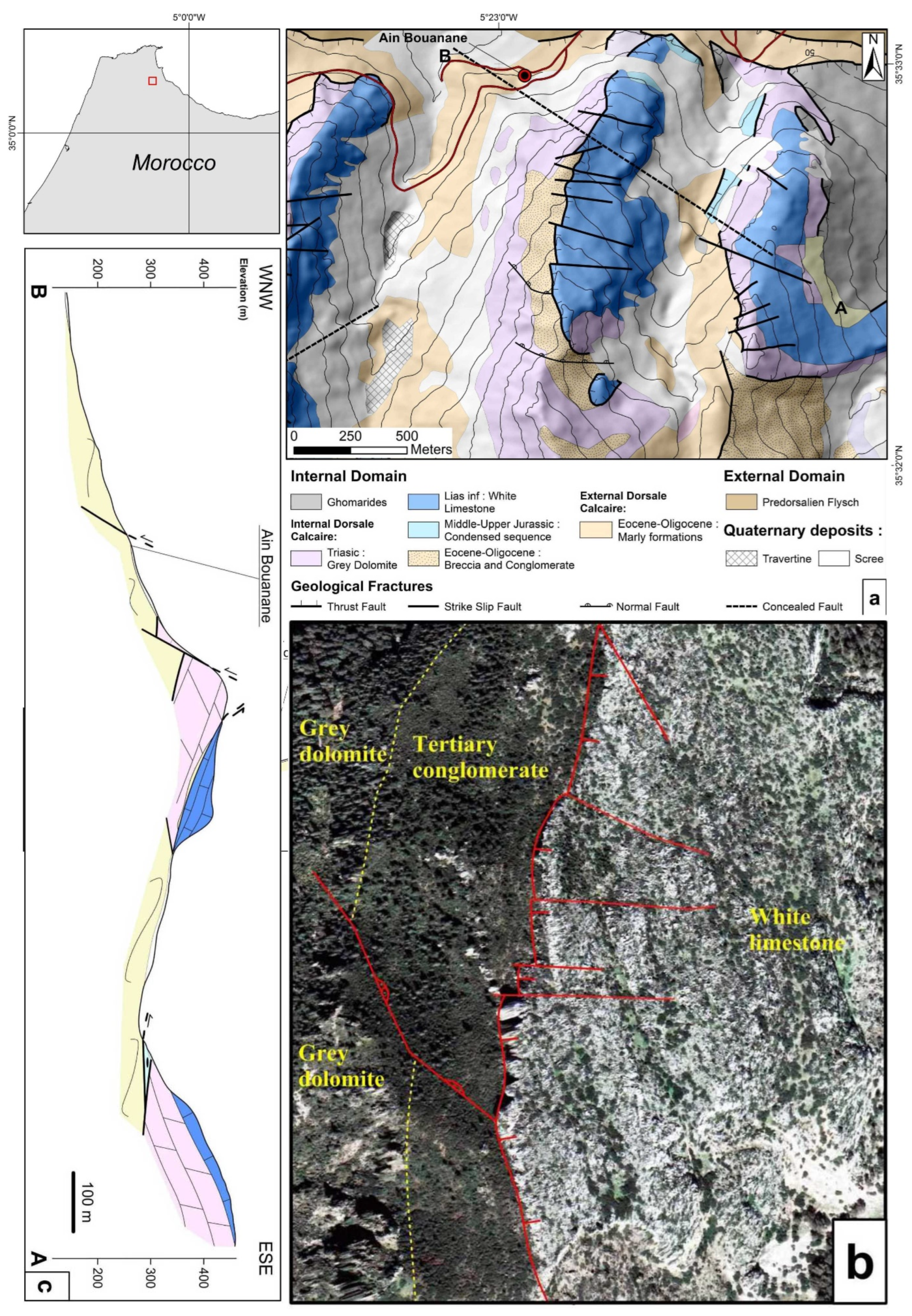
2.1. Geological and Geomorphological Setting

The Bouanane cliff is located immediately to the South of Tetouan (Figure 1a). From a morphological point of view, it is characterized by a subvertical topography with an elevation difference of about 120 m. The geological material outcropping at the site is attributed to the Dorsale Calcaire structural unit, which is mainly formed by thick layers of Triasic and Jurassic carbonate rocks with a fairly developed Tertiary sedimentary cover [30,31,32,33]. This structural unit is considered a unique morphostructural domain that is essentially constructed by carbonate rock ridges consequential to the thrust sheet structure of the Rif Cordillera [34].

However, the structure of the Bouanane cliff is not attributed to these N-S oriented thrust faults. It is, in fact, the result of late Miocene to Pliocene extensional deformation, which reactivated the E-W striking, right-lateral, strike-slip Tetouan accident into a normal faulting system (Figure 1b). This system of strike-slip faults, mainly N50° to N90°, is believed to be responsible for the morphogenesis of the Tetouan water-gap [35,36]. The field observations and visual interpretation of the aerial photographs allow for the mapping such structures to the south of the Bouanane site. These aerial photographs show that the Bouanane ridge is formed by thick limestone and dolostone strata that are affected by the E-W strike-slip faults (Figure 1). Using the thick strata as a reference mark, the right-lateral motion of the faults can be clearly distinguished. The Bouanane cliff is also considered to be the result of complex right-lateral normal faulting that cuts the Bouanane ridge short to the north. On the field, one can also observe a dense tectonic joint network striking mainly N130° to N160°, which split the massive carbonate rocks into multiple metric blocs.

2.2. Rockfall Occurences in the Bouanane Site

In Northern Morocco, which is part of the Mediterranean peripheral chains, several rockfall and rock avalanche occurrences have had pronounced consequences. The sites subject to such phenomena include the village of Ametrass [37], El Onsar village north of Tetouan [38] and the cliff of Bouanane which is the subject of the present paper. The common characteristics between the above-mentioned cases is the damage caused due to the presence of human dwellings and infrastructures in the piedmont of these cliffs and the lack of protection structures against rockfalls. In Bouanane, three previous events have caused material damage without any casualties. The first, which dates back to 1994, did not cause any damage despite the large size of the detached boulder. The second, unlike the first, damaged two parked vehicles in 2011, despite the relatively smaller size of the boulders involved. The most recent occurrence, which took place on 1 December 2018, caused damage to the decorative fence surrounding a car parking spot and stopped at the doorstep of a coffee shop. The latter event will be investigated in detail. The trajectory and some of the impact points will also be used as validation data to assess the accuracy of the simulation models produced using the three DEMs with different resolutions.

3. Materials and Methods

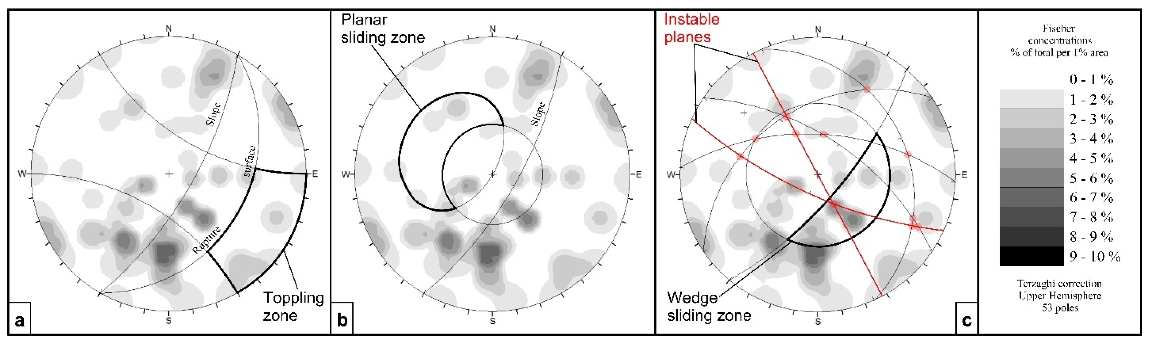
3.1. Stability of the Bouanane Cliff

Before presenting the simulation models, we will attempt to study the detachment mechanisms and assess the stability of the Bouanane cliff. To do so, the strike and dip of 56 tectonic joints were measured during several field surveys conducted in 2017 and 2018. This helps to identify the major joint directions/families in the area and their geometrical association with the cliff’s morphology.

Regarding the stability of the Bouanane cliff, the SMR (slope mass rating) index [39] was calculated using the automated SMRTool beta 1.10 [40]. Although this classification constitutes a good tool for assessing the stability of the rocky slopes, several modifications were developed to further enhance its performance in heterogeneous or anisotropic slopes [41]. Given the important elevation difference of the Bouanane cliff, we opted for the Chinese adaptation CSMR [42], which integrates the elevation difference of the investigated slope into the calculation Formula (1)

CSMR = E · RMR + L (F1 · F2 · F3) + F4

(1)

where E = 0.43 + 0.57 (80/elevation difference), RMR (rock mass rating) is the Beniawski index [43], F1, F2, F3 and F4 are the correction parameters and L is an index that reflects the state of the geological fractures affecting the cliff [39].

L (between 0.8 and 1) is the index that reflects the state of the geological fractures affecting the cliff. A value of 0.8 is generally assigned where the involved geological fractures are large-scale metric or decametric joints, and a value of 1 in the opposite case. In this study, the former value is adopted. The height of the slope used in this calculation was 65 m, while its dip and dip direction were 50° and N315, respectively. As the general slope was natural, the F4 parameter value used was 15.

3.2. Detachment Mechanisms

To decide which detachment mechanism controls the rockfall dynamics at the study area, dip and dip direction measurements were used to graphically estimate the probability of toppling (T), planar sliding (P) and wedge sliding (W) in Bouanane, using the Goodman method [44]. To estimate the risk of toppling, we counted the number of joint planes poles that were projected inside the zone and delimited by the friction cone (trend = slope dip direction + 90, plunge = 0; and angle = 60) and the sliding limit surface (dip = slope dip-friction angle; dip direction = slope dip direction). Such joints have a high potential for producing rockfalls through toppling. The more poles there are, the greater the risk. To determine which joint planes may cause planar sliding, the density of the poles located outside the friction cone (trend = 0, plunge = 90 and angle = friction angles) and delimited by the daylight envelope of the slope, were visually estimated, which reflected the probability of rockfall occurrence by planar sliding. For the last mechanism, the intersection points between the average planes of each joint family, located within the zone delimited by the slope and the friction cone (trend = 0; plunge = 90; and angle = 90 friction angle), indicated the potentially unstable planes that may produce wedge sliding. The quantification of this risk was also achieved through a graphical estimation of the density of unstable joint families.

3.3. Preparation of Topographic Data

In this study, we will use five DEMs with varying spatial resolution and vertical accuracies. The first was downloaded from the USGS’s Earth Explorer platform (https://earthexplorer.usgs.gov/, accessed on 3 December 2022). It is a 1 arc second (approximately 30 meter) resolution DEM produced by the Shuttle Radar Topography Mission (SRTM). This dataset has the lowest resolution. The second DEM (5 m resolution) was generated using elevation contours derived from the 1:25,000 topographic map of the study area. The elevation contours were digitized manually and an interpolation of the data was performed.

Another high-resolution digital surface model (DSM) (11 cm) was generated using a set of UAV-derived aerial photographs. The UAV used was a DJI Phantom 4 drone equipped with a Global Positioning System (GPS) module, with a vertical accuracy of 0.1 m and a horizontal accuracy of 0.3 m. The camera used for capturing the aerial photographs is a 1/2.3″ CMOS camera with a total number of effective pixels of 12.4 M. Further information regarding the hardware specifications and acquisition parameters is presented in Supplementary Table S1.

The processing chain that was followed to obtain this model first consisted of eliminating the bad quality tie points and introducing 310 ground control points (GCPs) (Supplementary Figure S1) to optimise the initial point cloud before generating the 3D dense points cloud and the digital surface model (DSM). The GCPs that were exploited to enhance the model were acquired by the Urban Agency of Tetouan using a dual frequency SpectraSP60 D-GPS in static mode, with a spatial accuracy of +/− 5 cm. The tool used to perform the structure-from-motion (SFM) analyses in this study was the open source MicMac photogrammetry software that is freely available at https://micmac.ensg.eu, accessed on 3 December 2022.

One of the main difficulties that we encountered in this study, was the presence of a dense forest canopy in the surveyed area, which needed to be filtered out in order to avoid creating artificial barriers in the simulation model. To do so, several post-processing steps were performed to correct the altitude values of the forest canopy tie points. The correction methods frequently deployed were based on the use of GCPs that were measured using precise ground positioning techniques. These were subsequently used to correct the elevation values for the areas with dense vegetation [45], a near-infrared based filtration of the points corresponding to the forest canopy [46] and the use of a ground-based scanner (TLS) [47]. LiDAR imagery was an alternative, but its cost was higher and it was consequently not considered in this study for budgetary reasons. In addition, obtaining permits for the use of this technique in our study area was not possible, so we opted for the SFM alternative.

To correct the forest canopy points, we used the first approach where 186 of the 310 GCPs, provided by the Urban Agency of Tetouan (Supplementary Figure S1) and measured using differential GPS, were used to calculate the mean elevation of the pine tree canopy in the study area. This was achieved through subtracting the interpolated elevation surface, calculated using the GCPs, from the canopy elevation raster provided by the UAV-derived model. The average tree height was found to be around 9.23 m with a standard deviation of 2.74 m. This low variance was due to the fact that all the trees at the site were planted in the same year (1969) as part of a reforestation effort by the Moroccan government and, therefore, have a more or less similar size. After the subtraction was done, the surface was smoothed using a majority filtering algorithm that replaced each cell value based on the twelve contiguous neighboring cells (Figure 2).

The resolution of the UAV model was downgraded to 1 m to avoid memory allocation errors in the Rocpro 3D simulation software (Figure 3). Two other models were derived from the UAV DEM with spatial resolutions of 2 m and 3 m. Along with the other two DEMs (Figure 3), the topographic data was prepared for simulation purposes. An additional 102 GCPs (Supplementary Figure S1B) acquired from the same agency were used to assess the vertical accuracy of the used DEMs and compare them to one another. The vertical error distribution presented in Figure 3D shows that the 1 m and 3 m DEMs are very similar in terms of the mean error values, the standard deviation and the overall distribution. Surprisingly, the 2 m DEM was less accurate than the 3 m one. Finally, the 5 m and 30 m DEMs were shown to present the highest mean error values and also presented a more uniform error distribution compared to the UAV-derived DEM.

3.4. D trajectory Simulation

The software deployed in this study (RocPro3D) used physical parameters such as rebound (restitution coefficient and lateral deviation), rolling (friction coefficient, limit velocity) and transition parameters of the soil and boulders in order to estimate the possible propagation trajectories, energy, velocity and impact points. The approximate values of these parameters for bare and densely vegetated dolomite scree deposits and loose soils were taken from the typical values table available in the Help section of the website (www.rocscience.com, accessed on 3 December 2022), which is based on previous experimental research [21,23]. This research estimated the parameter range for soils that are similar to the ones present at Bouanane. Although the individual trees were not integrated into the 3D mesh, their effects on the soil parameters were also included in these estimation efforts. The soils covered by the forest canopy in our study area were considered densely vegetated soils and, therefore, their corresponding parameters were adopted. With respect to the trajectory estimation, we chose the rigid body approach of the RocPro3D simulator for a maximum output of 50 simulated trajectories. The boulder diameter used was that of the biggest dolomite boulder that fell in 2018. This was done in order to validate our simulation results using the field data, which cannot be achieved if the boulder sizes are different.

3.5. Statistical Analyses

While visual interpretation of the results allowed for a comparison the three models used in this study, numerically deploying statistical techniques quantified the difference, which provided more solid evidence regarding the degree of significance of our findings. Therefore, we first attempted to assess the horizontal error distribution through a histogram plot of the distance to real trajectory of each of the five simulated models. To do so, the polyline shapefiles representing the simulated trajectories were first rasterized using a GIS tool. Then, the latter were used to compute the Euclidean distance separating the centre of each pixel from the field trajectories. Generally speaking, an error range of 0 to 2 m is considered good since all of the potential rockfall targets at Bouanane are objects wider than 4 m (e.g., buildings, cars, café terraces, etc.). Therefore, the probability that the simulated boulder missed its real target is low for such an error range.

Additionally, we prepared a box plot of the runout simulation results in order to graphically represent the simulated samples and compare them to the field reference values. Subsequently, the Kruskal–Wallis non-parametric test [48] was performed to compare the three produced simulations, since the data were clearly non-normally distributed [48]. The input variables introduced to the Kruskal–Wallis algorithm were the simulated velocity, energy and bounce height, obtained from our 3D simulation effort. The null hypothesis for such a test was that all five models would be equal and that the observed difference would not be statistically significant. Dunn’s (PostHoc) test [49] was also performed to point out which of the models were similar and which were different based on a pairwise comparison approach.

3.6. Morphometry of Scree Pebbles and Boulders

To study the morphometry of the piedmont deposits at Bouanane, the length (a), width (b) and thickness (c) of 1749 pebbles were measured at 11 sampling stations during several field investigations (Supplementary Tables S2 and S3 and Figure S2). The same measurements were taken for 55 boulders, the locations of which were determined using a GPS tool (Supplementary Tables S4 and S5). For the boulders, the measured values were projected onto the Sneed and Folk ternary diagram [50] using the Hockey coordinate system [51]. The latter was adopted for its simplicity. The computer tool used in this study was "Tri-plot" (https://www.lboro.ac.uk/microsites/research/phys-geog/tri-plot/index.html, accessed on 3 December 2022). The results should allow for the studying of the morphology of the pebbles and boulders and consequently the characterization of their size and shape distributions. For the scree pebbles, the value of the ’b’ axis was used to generate a cumulative frequency plot in order to determine the statistical mode of the samples. This allowed for the determination of the physical soil parameters of the scree deposits layers using the above-mentioned reference values table.

4. Results

4.1. Stability of the Bouanane Cliff and Detachment Mechanisms

The geometric attributes and geomechanical measurements of the seven tectonic joint families identified in the study area were used in CSMR calculations. Our results yielded a value of around 70 in the study area (

Table 1. CSMR analysis results for the Bouanane cliff.

Joints Family *	RMR	α (j)	β (j)	α (s)	β (s)	H (m)	L	E	F1	F2	F3	F1*F2*F3	CSMR
F1	40.12	225	55	315	50	65	0.85	2.23	0.15	1	0.65	0	89.5
F2	27.32	270	66	315	50	65	1	2.23	0.22	0.98	1.19	−0.25	61
F2’	27.32	90	66	315	50	65	1	2.23	0.22	1	−2.15	−0.47	60
F3	34.6	315	54	315	50	65	1	2.23	1	0.96	−4.68	−4	73
F4	39.4	180	65	315	50	65	0.9	2.23	1	0.96	−1.76	−0.39	88
F5’	27.1	135	80	315	50	65	1	2.23	1	1	−25	-25	35
F5	27.1	315	80	315	50	65	1	2.23	1	0.99	−0.64	−0.63	60
F6	39.33	225	85	315	50	65	0.8	2.23	0.15	1	−25.31	−4	85
F7	39.3	0	63	315	50	65	1	2.23	0.22	0.97	−1.47	−0.31	87
												Average =	70

* RMR (rock mass rating). α (j) joint dip direction. β (j) joint dip. α (s) slope dip direction. β (sj) slope dip. H (m) height of the slope. L (index that reflects the state of the geological fractures affecting the cliff). E = 0.43 + 0.57 (80/elevation difference). F1, F2 and F3 are the correction parameters of Romana.

), which means that the Bouanane cliff can be considered as a class II slope according to the Romana classification [39]. In terms of the stability, this class was deemed stable with few rockfall occurrences. Their temporal probability should not exceed 0.2 according to the same classification, which was in accordance with the testimonies and accounts of the local people.

According to our field surveys and the UAV high-resolution images, the main joints family responsible for the segmentation of the cliff into smaller metric blocks is the conjugated WNW-ESE to NW-SE tectonic joints (Figure 4). Together, they form X-shaped lines that intersect the cliff at a 60° to 70° angles.

Regarding the boulder detachment mechanisms, the Goodman analysis [44] performed in the Bouanane cliff (Figure 5) showed that wedge sliding processes had a high occurrence probability. This was explained by the presence of the above-described dense joint network, the orientation of which was quasi-orthogonal to the main scarp direction. As for the other possible detachment styles, the probability of planar sliding and toppling were found to be low (<5%) due to the low frequency of NE-SW oriented tectonic joints (Figure 4 and Figure 5).

4.2. Investigation of the December 2018 Event

Our field surveys that were conducted immediately after the rockfall event of 1 December 2018, allowed us to draw the trajectory of three detached boulders (Figure 6a). At the source area, fresh impact holes were identified (Figure 6b). These holes were not very deep but were large enough to suggest a significant impact force that exposed the dark quaternary soil layers. Immediately below the source area, fresh mechanical injuries were seen on some trees that did not show any signs of impact prior to the event (Figure 6c,d). The fresh yellowish color of the impacts on the Pinus halepenesis trunks also indicated the freshness of the injuries, since old impacts on these pine trees tend to darken very quickly due to the hardening of the resin secretions [52]. At the bottom of the steep slope, the three detached boulders landed separately. The two that reached the inhabited zone were easy to locate since they left behind clear impacts on manmade structures (Figure 6e,f). However, the third boulder was more difficult to find since it was stopped by an older and bigger buried boulder (Figure 6g). The latter boulder was distinguished from the older boulders by the presence of reddish wood and resin stains on its surface. The size of all three boulders was measured on the field. Their diameters were found to be 1.2 m, 1.8 m and 1.5 m, respectively, indicating a more or less similar size.

4.3. Significance of the 2018 Event

The diameter-frequency distribution (Figure 7a) for the 55 boulders measured below the source area, showed that 0.5-to-2-meter large boulders constituted the dominant category in the study area (Figure 7a). Given that 26 of the 55 boulders belonged to the 1 to 1.5 m category (Figure 7a), the rockfall event of December 2018 can be considered typical of the Bouanane site. In fact, with a boulder diameter ranging from 1.2 to 1.8 m, the detached boulders were “coarse” according to the [53] classification, with this category being the most dominant in the study area.

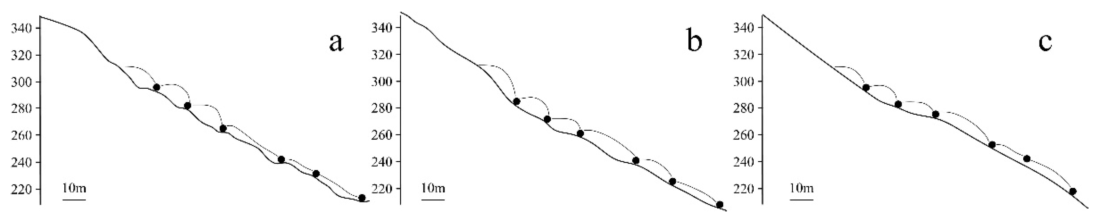
4.4. Rockfall Trajectory Simulation and Back-Analysis

The trajectory simulations produced using the five above-mentioned DEMs are shown in Figure 8. The first model, which used the 1 m resolution DEM as the topography input, produced complex trajectories that corresponded more or less to the field observations (Figure 8a). Of the different calculated trajectories, a significant portion did not reach manmade structures, while the rest either stopped at the coffee shop impacted by the 2018 event or continued further to impact other buildings downhill. As can be seen in Figure 8, the runout distances rarely exceed that of the longest documented path (Figure 8f), suggesting a reasonably accurate depiction of the real event. The 2 m (Figure 8b) and 3 m (Figure 8c) DEM simulations were more or less similar trajectories with slightly wider invasion zones and longer runout distances. These differences, although small, produced a significant runout calculation error according to Figure 8f, since the runout value range did not intersect that of the real trajectories.

The fourth and fifth models, which used the 5 m and 30 m DEMs as the topographic data, respectively, produce smoother and longer trajectories that did not follow the paths of the 2018 rockfall occurrence (Figure 8d,e). For the mid-resolution model, most if not all calculated runouts significantly exceeded the observed values with no boulders stopping before they reached the inhabited area (Figure 8f). As for the low-resolution simulation, the runout values were even bigger, with all the boulders reaching areas that presented no signs of any recent occurrences (Figure 8e,f). The simulated trajectories of the fifth model also missed the coffee shop that was affected by the recorded 2018 rockfall, yielding a deformed representation of the real event. The consequences of such errors are discussed in Section 5.

In terms of the horizontal error distribution, the distance to real trajectory histogram presented in Figure 9 confirmed the visual interpretation results. According to this histogram, the percentage of the 0 to 2 m error range (good error range) negatively correlated with the DEM resolution, which means that the lower the resolution, the greater the overlap between the simulated and real invasion zones. Conversely, the >25 m error range was dominated by the 30 m model (Figure 9), which also correlated well with our visual interpretation of the results. Consequently, the high spatial errors were reverse proportional to the resolution of the data where coarser models produced significantly worse results relative to the real trajectories.

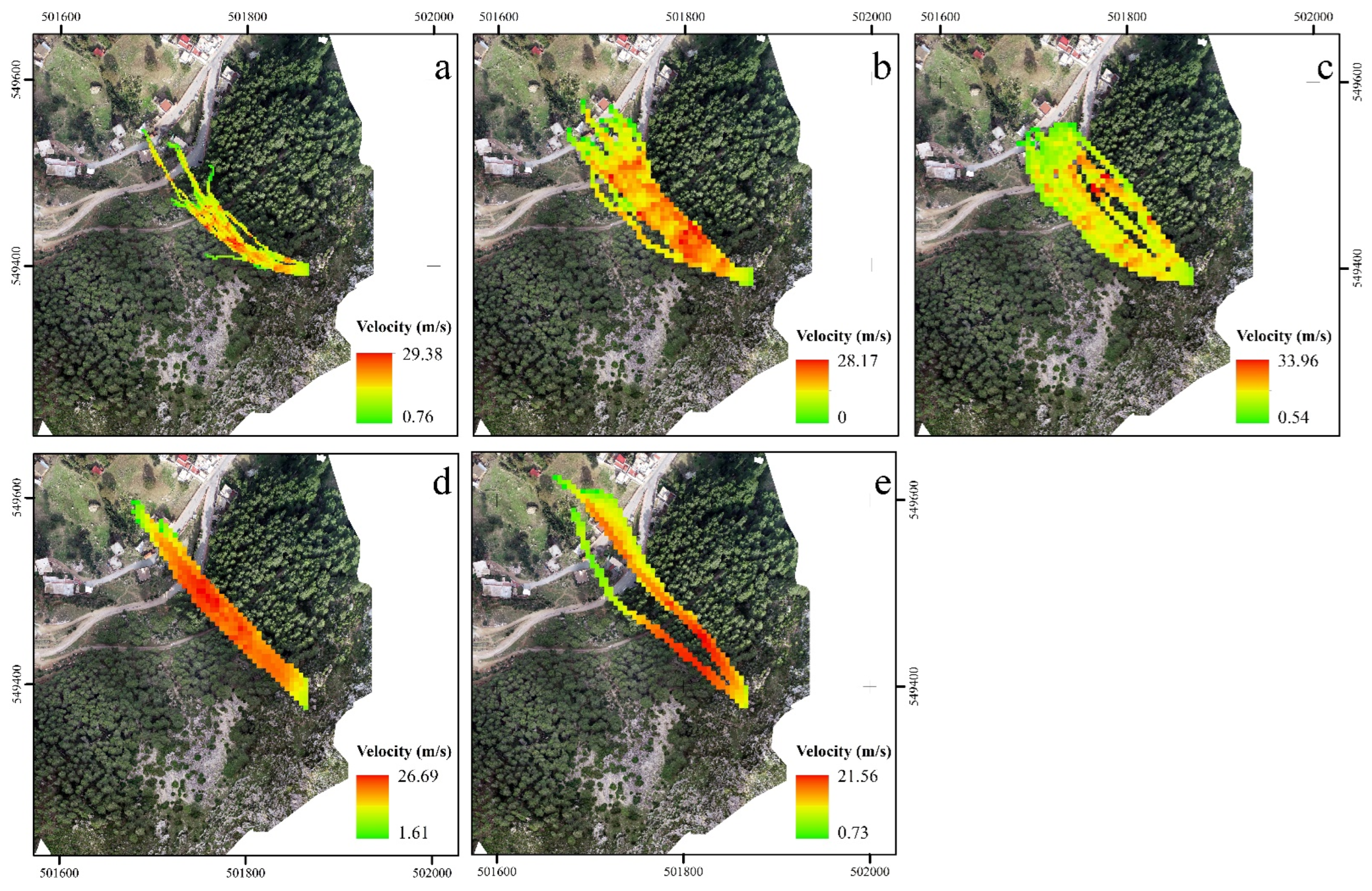
4.5. Energy and Velocity Simulation

The simulated velocity values showed that the 3 m resolution DEM produced the widest range of values. It also yielded the highest velocity with a maximum of 33.96 m/s compared to a maximum of only 29.28 m/s, 28.17 m/s, 26.69 m/s and 21.56 m/s for the other models (Figure 10). However, when the simulated boulders reached the manmade structures, the velocity for the first and third models (Figure 10a,c) was low in comparison to the rest, which presented higher velocities reaching up to 20 m/s. By comparing these values to the impacts observed on the field, the latter appeared to correspond more to the high-resolution simulation since the damage was mainly aesthetic and indicated low-velocity impacts. As for the 2 m and the medium and low-resolution models, they were found to exaggerate the true velocity downhill. Similar remarks can be given regarding the spatial distribution of the energy values (Figure 11).

In terms of the percentage, the spatial distribution of both the velocity and energy values differs, where low to medium values tend to cover the most area in the 1 m and 3 m models, while high values dominate in the other models, especially the 5 m model. The probable reasons for this are explained in Section 5.

This spatial distribution difference was well attested by the Kruskal–Wallis test results (

Table 2. Kruskal–Wallis test results.

Dependent Variable	Kruskal–Wallis Test
	H	p-Value
Velocity	470.035	<0.001
Energy	1387.988	<0.001
Bouncing height	498.55	<0.001

) that showed a low P-value output (<0.0001). Given a threshold of 0.05, these findings proved that the observed spatial distribution difference was statistically significant. The pairwise Dunn test also yielded a similar output for the velocity and energy, with P-values largely inferior to 0.05 (<0.001) (

Table 3. Dunn’s (Post Hoc) test results.

Dependent Variable	DEMs	p-Value	Dependent Variable	DEMs	p-Value
Velocity	1–2 m	<0.001	Bouncing height	1–2 m	<0.001
	1–3 m	<0.001		1–3 m	<0.001
	1–5 m	<0.001		1–5 m	<0.001
	1–30 m	0.002		1–30 m	<0.001
	2–30 m	<0.001		2–3 m	<0.001
	2–3 m	0.237		2–5 m	<0.001
	2–5 m	<0.001		2–30 m	<0.001
	3–5 m	<0.001		3–5 m	<0.001
	3–30 m	<0.001		3–30 m	<0.001
	5–30 m	<0.001		5–30 m	<0.001
Energy	1–2 m	<0.001
	1–3 m	<0.001
	1–5 m	<0.001
	1–30 m	<0.001
	2–3 m	<0.001
	2–5 m	<0.001
	2–30 m	<0.001
	3–5 m	<0.001
	3–30 m	<0.001
	5–30 m	<0.001

), with the exception of the 2 m and 3 m DEMs, which appeared to have similar velocity distributions.

5. Discussion

5.1. How the DSM Resolution Impacts the Rockfall Numerical Simulations

In the rockfall simulations, the researchers sought to model the geometry of the possible boulder trajectories, which allowed for distinguishing between hazardous and safe areas, the runout values that determine how far a detached boulder can travel and the velocity and energy of boulders once they descend the slope. The DEM resolution influenced all the above-mentioned aspects of the rockfall research. In fact, [18] declared that the use of coarser topographic grids translated into a decreased variability in the computed trajectories, higher mean velocity values and lower bounce heights due to the smoother geometry of the DEM. Similar remarks were reported in a more recent study by [19] who showed that higher resolution input data exhibited more complex trajectory shapes that agreed more with historical inventories. In our case study, the UAV-derived 1 m DEM yielded more complex geometries that agreed well with our field observations (Figure 11a). The invasion zone produced by this high-resolution model was also smaller but had more variability in terms of the shape and length of the simulated trajectories, which was similar to the previous findings.

In the previous research, the runout extent was also shown to change significantly in some cases [19,20] and stayed the same in others [18]. This effect can be explained by the roughness of the terrain which was demonstrated to be proportional to the runout variability using anecdotal evidence [20]. In this work, the mean runout for the high-resolution model was lower than those obtained using coarser DEMs. In fact, it appeared that the lower the resolution of the topographic data, the longer a boulder will travel downhill. Such results were due (in our study as well) to the rugged and bumpy topography of the site, which translated into large differences between the DEMs used in this study. However, the effects of the slope roughness on the travel mode of rockfalls depends on the slope ratio as well. [54] showed that while rough surfaces tend to promote higher velocity rockfalls in steep slopes, their influence is reversed in gentler slopes due to a loss of energy on impact (Figure 10). This explains why the highest velocity calculated in this case study was given by the higher resolution DEMs near the source area, despite them presenting the shortest runouts. Consequently, the appropriateness of a DEM for use in a simulation can be summarized in its ability to depict the micro-topographic geometries, such as micro terraces, small holes and micro-ridges. Such small but significant details regarding the topography of a given slope can change the outcome of a rockfall simulation depending on the steepness of the hillslopes and its real shape. In Bouanane, the topography was dominated by small convex uphill surfaces, which explained why the simulated velocity in this segment of the slope was higher in the high-resolution model compared to the medium and low-resolution models (Figure 12a). Larger concave downhill surfaces were accurately represented by the 1 m DEM but appeared smoother in the coarser DEM, resulting in shorter runouts in the former and longer trajectories in the latter (Figure 12b,c).

In addition to the roughness, the elevation of the unstable cliff/slope determined how big the effect of the DEM resolution was on the simulation results, especially the runout distance. The experimental results published by [18] showed that the runout did not change significantly when using different DEM resolutions. However, in cases where the source area belongs to the domain of middle slopes and ridges, such as the case of the Bouanane cliff, the resolution and detailed depiction of the topography determined mostly where the boulders stop. This was because the valley floor was a flat surface, the shape of which does not vary from one DEM to the other. Therefore, the falling boulder stopped at approximately the same area due to an absence of a horizontal component of acceleration. In addition, the moving object lost energy quickly regardless of the initial impact force. Nevertheless, when the topography was inclined, the stopping position was more sensitive to the acceleration component and friction forces that mainly depended on the shape of the impact surface. As such, the existence of micro topography features became more relevant to the results. For instance, the 1 m, 2 m and 3 m DEMs adopted in this study produced significantly different invasion zones and runout distributions despite being derived from the same techniques. The reason for this was the loss of the microtopographic details mentioned above.

5.2. Impact of the Simulation Results on the Hazard Assessment and Prevention Efforts

When an area is revealed to be hazardous, various solutions are implemented to reduce the vulnerability of constructions to rockfalls. Such protection countermeasures are either natural (e.g., tree barrier effect, etc.), quasi-natural (e.g., building embankments and ditches), structural (e.g., monolithic rockfall protection galleries) or flexible (e.g., fences and other flexible barriers). The proper design and dimensions of such protection structures varies depending on the geometry of the slope, the simulated energy of the boulders, the impact load and the bouncing height in the runout area [55]. Since such values are generally obtained from numerical models, the above-presented effects of the topography on the simulation results plays a major role in rockfall prevention efforts. For instance, the construction of rockfall protection fences in Bouanane (which are deemed the most appropriate technique due to the geometry of the slope) required information regarding the runout, bouncing height and the most probable targets for potential future events. In the coarse resolution simulations, the output was shown to differ significantly from the real trajectory drawn on the field. For the 5 m DEM model, the inaccuracies were mainly due to the shape of the modeled trajectories, which deviated significantly from field data. In addition, the velocity and energy values (Figure 10 and Figure 11) were exaggerated near the real target area compared to the slight impacts observed (Figure 6). As for the 30 m model, it was shown to miss the most probable trajectory, stopping far away from the observed rockfall path (Figure 6). Therefore, if such models were to be used, they would induce significant positioning errors. Conversely, the 1 m model presented a reasonably accurate invasion zone that corresponded to the reality of the field, which could be used for hazard zonation mapping and rockfall prevention efforts.

Regarding the bouncing height distribution for the modeled trajectories, the 1 m and 2 m models appeared to present the highest uphill values (Figure 13a,b) compared to the coarse models where the boulders kept rolling downhill (Figure 13d,e). Although the detached boulders of the 2018 event did not leave behind evidence of high bouncing, old broken tree stems were hit at a ground elevation of 2 to 3 m (Figure 13g). The area where these trees were found corresponded to a clear land in the middle of the forest (Figure 13f), where the modeled trajectories revealed the highest bouncing heights. The implications for such variation are significant, given that a future protection fence should absorb the energy of the falling rock and, therefore, needs to be as high as or higher than the bouncing boulder itself. As such, the underestimation of the bouncing by the medium and coarse resolution models could hinder the effectiveness of the rockfall protection structures if the engineers were to rely solely on such data.

5.3. How the DEM Resolution Improve the Results

Although it is obvious that higher resolution data improves the simulation results, the question of a threshold resolution for the rockfall simulations remains valid. In this study, we tested five DEMs with a resolution range of 1 to 30 metres, with some being practically unusable for achieving accurate rockfall modeling. While the improvement is very significant going from the lowest to the highest resolutions, the difference between the 1 m and 2 m DEMs is less obvious, especially in terms of the trajectory shape and invasion zone geometry. Therefore, we wonder if exceeding the 1 m resolution limit would have produced any significant improvement in our case study. Some results presented by [20], who worked on two different sites, clearly showed that the geomorphological setting of the study area determined how the resolution will influence the output. Therefore, such investigations need to be conducted in a variety of locations around the world to determine a “universal” DEM threshold for rockfall hazard modeling under different geomorphological circumstances. Failling to do so may lead to large errors in many models that still use coarse DEMs. This matter will be more significant in developing countries where high-resolution topographic data is scarce and the investment in data acquisition technology is low.

6. Conclusions

Based on our findings, we believe that low-resolution DEMs are unsuitable for site specific rockfall simulations. Moreover, medium and coarse-resolution topographic data also induce large positioning and geometric errors that degrade the quality of a simulation and hinder its usability for prevention and protection efforts. The results of this paper suggest that high-resolution DEMs are required to produce reasonably accurate simulation models, with trajectory shapes, invasion zones and runout areas that agree well with field observations. This is especially true for areas belonging to the domain of middle slopes and ridges, such as the case of the Bouanane cliff, where the microtopographic features determine the simulation output. Although such data are not available worldwide, the use of new remote-sensing technology such UAVs can solve this problem and provide the accurate data needed for such studies. This technology is low cost, which should encourage its use especially when we consider the significant difference it has with respect to the accuracy of the output. However, fieldwork must always constitute the reference data, which allows for the calibration and validation of the simulation no matter the accuracy of the input.

References

1. Cruden, D.M.; Varnes, D.J. Landslide Types and Processes, Special Report, Transportation Research Board, National Academy of Sciences. U. S. Geol. Surv. 1996, 247, 36–75. [Google Scholar]
2. Guzzetti, F.; Reichenbach, P.; Ghigi, S. Rockfall Hazard and Risk Assessment Along a Transportation Corridor in the Nera Valley, Central Italy. Environ. Manag. 2004, 34, 191–208. [Google Scholar] [CrossRef]
3. Schweigl, J.; Ferretti, C.; Nössing, L. Geotechnical Characterization and Rockfall Simulation of a Slope: A Practical Case Study from South Tyrol (Italy). Eng. Geol. 2003, 67, 281–296. [Google Scholar] [CrossRef]
4. Gunzburger, Y.; Merrien-Soukatchoff, V.; Guglielmi, Y. Influence of Daily Surface Temperature Fluctuations on Rock Slope Stability: Case Study of the Rochers de Valabres Slope (France). Int. J. Rock Mech. Min. Sci. 2005, 42, 331–349. [Google Scholar] [CrossRef]
5. Abellán, A.; Vilaplana, J.M.; Calvet, J.; García-Sellés, D.; Asensio, E. Rockfall Monitoring by Terrestrial Laser Scanning-Case Study of the Basaltic Rock Face at Castellfollit de La Roca (Catalonia, Spain). Nat. Hazards Earth Syst. Sci. 2011, 11, 829–841. [Google Scholar] [CrossRef] [Green Version]
6. Sarro, R.; Mateos, R.M.; García-Moreno, I.; Herrera, G.; Reichenbach, P.; Laín, L.; Paredes, C. The Son Poc Rockfall (Mallorca, Spain) on the 6th of March 2013: 3D Simulation. Landslides 2014, 11, 493–503. [Google Scholar] [CrossRef]
7. Mateos, R.M.; Azañón, J.M.; Roldán, F.J.; Notti, D.; Pérez-Peña, V.; Galve, J.P.; Pérez-García, J.L.; Colomo, C.M.; Gómez-López, J.M.; Montserrat, O.; et al. The Combined Use of PSInSAR and UAV Photogrammetry Techniques for the Analysis of the Kinematics of a Coastal Landslide Affecting an Urban Area (SE Spain). Landslides 2017, 14, 743–754. [Google Scholar] [CrossRef]
8. Dellero, H.; El Kharim, Y. Rockfall Hazard in an Old Abandoned Aggregate Quarry in the City of Tetouan, Morocco. Int. J. Geosci. 2013, 4, 1228–1232. [Google Scholar] [CrossRef] [Green Version]
9. Asteriou, P.; Tsiambaos, G. Empirical Model for Predicting Rockfall Trajectory Direction. Rock Mech. Rock Eng. 2016, 49, 927–941. [Google Scholar] [CrossRef]
10. Chen, G.; Zheng, L.; Zhang, Y.; Wu, J. Numerical Simulation in Rockfall Analysis: A Close Comparison of 2-D and 3-D DDA. Rock Mech. Rock Eng. 2013, 46, 527–541. [Google Scholar] [CrossRef]
11. Glover, J.; Schweizer, A.; Christen, M.; Gerber, W.; Leine, R.; Bartelt, P. Numerical Investigation of the Influence of Rock Shape on Rockfall Trajectory. In Proceedings of the EGU General Assembly Conference Abstracts, Vienna, Austria, 22–27 April 2012; p. 11022. [Google Scholar]
12. Tarquini, S.; Vinci, S.; Favalli, M.; Doumaz, F.; Fornaciai, A.; Nannipieri, L. Release of a 10-m-Resolution DEM for the Italian Territory: Comparison with Global-Coverage DEMs and Anaglyph-Mode Exploration via the Web. Comput. Geosci. 2012, 38, 168–170. [Google Scholar] [CrossRef]
13. Cao, L.; Liu, H.; Fu, X.; Zhang, Z.; Shen, X.; Ruan, H. Comparison of UAV LiDAR and Digital Aerial Photogrammetry Point Clouds for Estimating Forest Structural Attributes in Subtropical Planted Forests. Forests 2019, 10, 145. [Google Scholar] [CrossRef] [Green Version]
14. Goodbody, T.R.H.; Coops, N.C.; White, J.C. Digital Aerial Photogrammetry for Updating Area-Based Forest Inventories: A Review of Opportunities, Challenges, and Future Directions. Curr. For. Rep. 2019, 5, 55–75. [Google Scholar] [CrossRef] [Green Version]
15. Jiang, S.; Jiang, C.; Jiang, W. Efficient Structure from Motion for Large-Scale UAV Images: A Review and a Comparison of SfM Tools. ISPRS J. Photogramm. Remote Sens. 2020, 167, 230–251. [Google Scholar] [CrossRef]
16. Westoby, M.J.; Brasington, J.; Glasser, N.F.; Hambrey, M.J.; Reynolds, J.M. ‘Structure-from-Motion’Photogrammetry: A Low-Cost, Effective Tool for Geoscience Applications. Geomorphology 2012, 179, 300–314. [Google Scholar] [CrossRef] [Green Version]
17. Žabota, B.; Repe, B.; Kobal, M. Influence of Digital Elevation Model Resolution on Rockfall Modelling. Geomorphology 2019, 328, 183–195. [Google Scholar] [CrossRef]
18. Agliardi, F.; Crosta, G.B. High Resolution Three-Dimensional Numerical Modelling of Rockfalls. Int. J. Rock Mech. Min. Sci. 2003, 40, 455–471. [Google Scholar] [CrossRef]
19. Lan, H.; Martin, C.D.; Zhou, C.; Lim, C.H. Rockfall Hazard Analysis Using LiDAR and Spatial Modeling. Geomorphology 2010, 118, 213–223. [Google Scholar] [CrossRef]
20. Bühler, Y.; Christen, M.; Glover, J.; Christen, M.; Bartelt, P. Significance of Digital Elevation Model Resolution for Numerical Rockfall Simulations. In Proceedings of the 3rd International Symposium Rock Slope Stability C2ROP RSS 2016, Lyon, France, 15–17 November 2016; pp. 15–17. [Google Scholar]
21. PFEIFFER, T.J.; BOWEN, T.D. Computer Simulation of Rockfalls. Bull. Assoc. Eng. Geol. 1989, 26, 135–146. [Google Scholar] [CrossRef]
22. Fisher, R.A. The Correlation between Relatives on the Supposition of Mendelian Inheritance. Earth Environ. Sci. Trans. R. Soc. Edinburgh 1919, 52, 399–433. [Google Scholar] [CrossRef] [Green Version]
23. Rammer, W.; Brauner, M.; Dorren, L.K.A.; Berger, F.; Lexer, M.J. Evaluation of a 3-D Rockfall Module within a Forest Patch Model. Nat. Hazards Earth Syst. Sci. 2010, 10, 699–711. [Google Scholar] [CrossRef]
24. Žabota, B.; Kobal, M. A New Methodology for Mapping Past Rockfall Events: From Mobile Crowdsourcing to Rockfall Simulation Validation. ISPRS Int. J. Geo-Inf. 2020, 9, 514. [Google Scholar] [CrossRef]
25. Lambert, S.; Bourrier, F. Design of Rockfall Protection Embankments: A Review. Eng. Geol. 2013, 154, 77–88. [Google Scholar] [CrossRef]
26. Schober, A.; Bannwart, C.; Keuschnig, M. Rockfall Modelling in High Alpine Terrain—Validation and Limitations/Steinschlagsimulation in Hochalpinem Raum—Validierung Und Limitationen. Geomech. Tunn. 2012, 5, 368–378. [Google Scholar] [CrossRef]
27. Pellicani, R.; Spilotro, G.; Van Westen, C.J. Rockfall Trajectory Modeling Combined with Heuristic Analysis for Assessing the Rockfall Hazard along the Maratea SS18 Coastal Road (Basilicata, Southern Italy). Landslides 2016, 13, 985–1003. [Google Scholar] [CrossRef]
28. Bonneau, D.A.; Hutchinson, D.J.; DiFrancesco, P.-M.; Coombs, M.; Sala, Z. Three-Dimensional Rockfall Shape Back Analysis: Methods and Implications. Nat. Hazards Earth Syst. Sci. 2019, 19, 2745–2765. [Google Scholar] [CrossRef] [Green Version]
29. Saroglou, C.; Asteriou, P.; Zekkos, D.; Tsiambaos, G.; Clark, M.; Manousakis, J. UAV-Based Mapping, Back Analysis and Trajectory Modeling of a Coseismic Rockfall in Lefkada Island, Greece. Nat. Hazards Earth Syst. Sci. 2018, 18, 321–333. [Google Scholar] [CrossRef] [Green Version]
30. Fallot, P. Essai Sur La Géologie Du Rif Septentrional; Imprimerie officielle: Rabat, Morocco, 1937; 553p.
31. Durand-Delga, M.; Hottinger, L.; Marcais, J.; Mattauer, M.; Milliard, Y.; Suter, C. Données Actuelles sur la Structure du Rif. Livre a la Mémoire du Professeur Paul Fallot; Société Géologique de France: Paris, France, 1961; pp. 339–422. [Google Scholar]
32. Didon, J.; Durand-Delga, M.; Kornprobst, J. Homologies Géologiques Entre Les Deux Rives Du Détroit de Gibraltar. Bull. Soc. Géologique Fr. 1973, 7, 77–105. [Google Scholar] [CrossRef]
33. Nold, M.; Uttinger, J.; Wildi, W. Géologie de La Dorsale Calcaire Entre Tétouan et Assifane (Rif Interne, Maroc). Notes Mémoires Serv. Géologique Maroc 1981, 233, 1–233. [Google Scholar]
34. El Gharbaoui, A. Note Preliminaire Sur l’evolution Geomorphologique de La Peninsule de Tanger. Bull. Société Géologique Fr. 1977, 7, 615–622. [Google Scholar] [CrossRef]
35. Romagny, A. Evolution des Mouvements Verticaux Néogènes de La Chaîne du Rif (Nord-Maroc): Apports d’une Analyse Structurale et Thermochronologique. Doctoral Dissertation, Université Nice Sophia Antipolis, Nice, France, 2014. [Google Scholar]
36. Benmakhlouf, M. Genèse et Évolution de l’accident de Tétouan et Son Rôle Transformant Au Niveau Du Rif Septentrional (Maroc) (Depuis l’oligocène Jusqu’à l’actuel). Ph.D. Thesis, Université Mohammed V, Faculté des Sciences, Rabat, Morocco, 1990. [Google Scholar]
37. Mastere, M. La Susceptibilité Aux Mouvements de Terrain Dans La Province de Chefchaouen: Analyse Spatiale, Modélisation Probabiliste Multi-Échelle et Impacts Sur l’aménagement & l’urbanisme. Ph.D. Thesis, Université de Bretagne Occidentale, Brest, France, 2011. [Google Scholar]
38. El Kharim, Y.; Darraz, C.; Hlila, R.; El Hajjaji, K. Écroulements et Mouvements de Versants Associés Au Niveau Du Col de Onsar (Rif, Maroc) Dans Un Contexte Géologique de Décrochement. Rev. Française Géotechnique 2003, 103, 3–11. [Google Scholar] [CrossRef] [Green Version]
39. Romana, M.R. A Geomechanical Classification for Slopes: Slope Mass Rating. In Rock Testing and Site Characterization; Elsevier: Amsterdam, The Netherlands, 1993; pp. 575–600. [Google Scholar] [CrossRef]
40. Riquelme, A.; Tomás, R.; Abellán, A. SMRTool Beta. A Calculator for Determining Slope Mass Rating (SMR). Universidad de Alicante. License: Creative Commons BY-NC-SA. 2014. Available online: http://personal.ua.es/es/ariquelme/smrtool.html (accessed on 2 May 2022).
41. Romana, M.; Tomás, R.; Serón, J.B. Slope Mass Rating (SMR) Geomechanics Classification: Thirty Years Review. In Proceedings of the 13th ISRM International Congress of Rock Mechanics, Montreal, QC, Canada, 10–13 May 2015; Volume 2015-MAY. [Google Scholar]
42. Chen, Z. Recent Developments in Slope Stability Analysis. In Proceedings of the 8th ISRM Congress, Tokyo, Japan, 25–29 September 1995. [Google Scholar]
43. Beniawski, Z.T. Rock Mass Classification in Rock Engineering Applications. In Proceedings of the a Symposium on Exploration for Rock Engineering 12, Johannesburg, South Africa, 1–5 November 1976; pp. 97–106. [Google Scholar]
44. Goodman, R.E. Introduction to Rock Mechanics; Wiley: New York, NY, USA, 1980; pp. 254–287. [Google Scholar]
45. Meng, X.; Shang, N.; Zhang, X.; Li, C.; Zhao, K.; Qiu, X.; Weeks, E. Photogrammetric UAV Mapping of Terrain under Dense Coastal Vegetation: An Object-Oriented Classification Ensemble Algorithm for Classification and Terrain Correction. Remote Sens. 2017, 9, 1187. [Google Scholar] [CrossRef] [Green Version]
46. Skarlatos, D.; Vlachos, M. Vegetation Removal from UAV Derived DSMS, Using Combination of RGB and NIR IMAGERY. In Proceedings of the ISPRS Annals of the Photogrammetry, Remote Sensing and Spatial Information Sciences, Riva del Garda, Italy, 4–7 June 2018; Volume 4. [Google Scholar]
47. Prokop, A.; Panholzer, H. Assessing the Capability of Terrestrial Laser Scanning for Monitoring Slow Moving Landslides. Nat. Hazards Earth Syst. Sci. 2009, 9, 1921–1928. [Google Scholar] [CrossRef] [Green Version]
48. Blanca Mena, M.J.; Alarcón Postigo, R.; Arnau Gras, J.; Bono Cabré, R.; Bendayan, R. Non-Normal Data: Is ANOVA Still a Valid Option? Psicothema 2017, 29, 552–557. [Google Scholar]
49. Dunn, O.J. Multiple Comparisons Using Rank Sums. Technometrics 1964, 6, 241–252. [Google Scholar] [CrossRef]
50. Sneed, E.D.; Folk, R.L. Pebbles in the Lower Colorado River, Texas a Study in Particle Morphogenesis. J. Geol. 1958, 66, 114–150. [Google Scholar] [CrossRef]
51. Hockey, B. An Improved Co_Ordinate System for Particle Shape Representation: NOTES. J. Sediment. Res. 1970, 40, 1054–1056. [Google Scholar] [CrossRef]
52. Perret, S.; Baumgartner, M.; Kienholz, H. Inventory and Analysis of Tree Injuries in a Rockfall-Damaged Forest Stand. Eur. J. For. Res. 2006, 125, 101–110. [Google Scholar] [CrossRef] [Green Version]
53. Blair, T.C.; McPherson, J.G. Grain-Size and Textural Classification of Coarse Sedimentary Particles. J. Sediment. Res. 1999, 69, 6–19. [Google Scholar] [CrossRef]
54. Wang, I.-T.; Lee, C.-Y. Influence of Slope Shape and Surface Roughness on the Moving Paths of a Single Rockfall. Int. J. Civ. Environ. Eng. 2010, 4, 122–128. [Google Scholar]
55. Abramson, L.W.; Lee, T.S.; Sharma, S.; Boyce, G.M. Slope Stability and Stabilization Methods; John Wiley & Sons, INC.: Hoboken, NJ, USA, 2001; Volume 706. [Google Scholar]
56. Rosenberg, D.; Shtober-Zisu, N. The Stone Components of the Pits and Pavements. In An Early Pottery Neolithic Occurrence at Beisamoun, the Hula Valley, Northern Israel; BAR International Series: Oxford, UK, 2007; pp. 19–34. [Google Scholar]
Figure 1. (a) Geological map of the study area. (b) Aerial photographs showing strike-slip faults affecting the Bouanane massif. (c) Geological cross section of the Dorsale Calcaire thrust sheets south of Tetouan.
Remotesensing 14 06205 g001
Figure 2. Processing chain of the UAV images.
Remotesensing 14 06205 g002
Figure 3. DEMs used for simulating the 2018 event. (A) UAV-derived DEM. (B) 5 m DEM. (C) SRTM 30 m DEM. (D) Vertical error distribution for the three DEMs used in this study.
Remotesensing 14 06205 g003
Figure 4. Major joint directions obtained from the field investigations and UAV images.
Remotesensing 14 06205 g004
Figure 5. Result of the Goodman analysis conducted on the Bouanane cliff. (a) Toppling analysis, (b) Planar slide analysis. (c) Wedge slide analysis.
Remotesensing 14 06205 g005
Figure 6. (a) Trajectories of the 2018 event projected over the UAV-derived orthoimage. (b) Boulder impact near the source area. (c) and (d) Mechanical injuries on the tree stems. (e) and (f) impact observed on manmade structures. (g) photograph showing a recently detached boulder with fresh resin and live wood stains on its surface and its supposed impact on a nearby tree.
Remotesensing 14 06205 g006
Figure 7. (a) Size-frequency distribution of boulders in the Bouanane site. (b) Boulders measured in the Bouanane site projected onto the Sneed and Folks (1958) diagram. The used classification for the boulders investigated in the study area is shown in Table S6 of the Supplementary Materials.
Remotesensing 14 06205 g007
Figure 8. Simulated rockfall trajectories using the 1 m UAV-derived DEM (A), the 2 m DEM (B), the 3 m DEM (C), the 5 m DEM (D) and the 30 m DEM (E). (F) Box plot of the runout distances obtained from the simulation models compared to the observed runouts of the 2018 event.
Remotesensing 14 06205 g008
Figure 9. Statistical distribution of the horizontal error for all five simulated models.
Remotesensing 14 06205 g009
Figure 10. Simulated rockfall velocity simulation in the Bouanane cliff obtained using the 1 m DEM (a), the 2 m DEM (b), the 3 m DEM (c), the 5 m DEM (d) and the 30 m DEM (e).
Remotesensing 14 06205 g010
Figure 11. Simulated rockfall energy simulation in the Bouanane cliff obtained using the 1 m DEM (a), the 2 m DEM (b), the 3 m DEM (c), the 5 m DEM (d) and the 30 m DEM (e).
Remotesensing 14 06205 g011
Figure 12. Theoretical 2D profiles of a rockfall event, drawn on a topographic profile extracted from the 1 m resolution DEM (a), the 5 m resolution DEM (b) and the 30 m resolution DEM (c).
Remotesensing 14 06205 g012
Figure 13. Bouncing height simulations produced using the 1 m DEM (a), the 5 m DEM (b) and the 30 m DEM (c). (d) UAV-derived orthoimage showing clear land (f) caused by repetitive rockfall events. (e) stem breakage (g) caused by an old rockfall occurrence.
Remotesensing 14 06205 g013