
Ongoing Development of the Bass Strait GNSS/INS Buoy System for Altimetry Validation in Preparation for SWOT

Abstract
:1. Introduction
2. Data
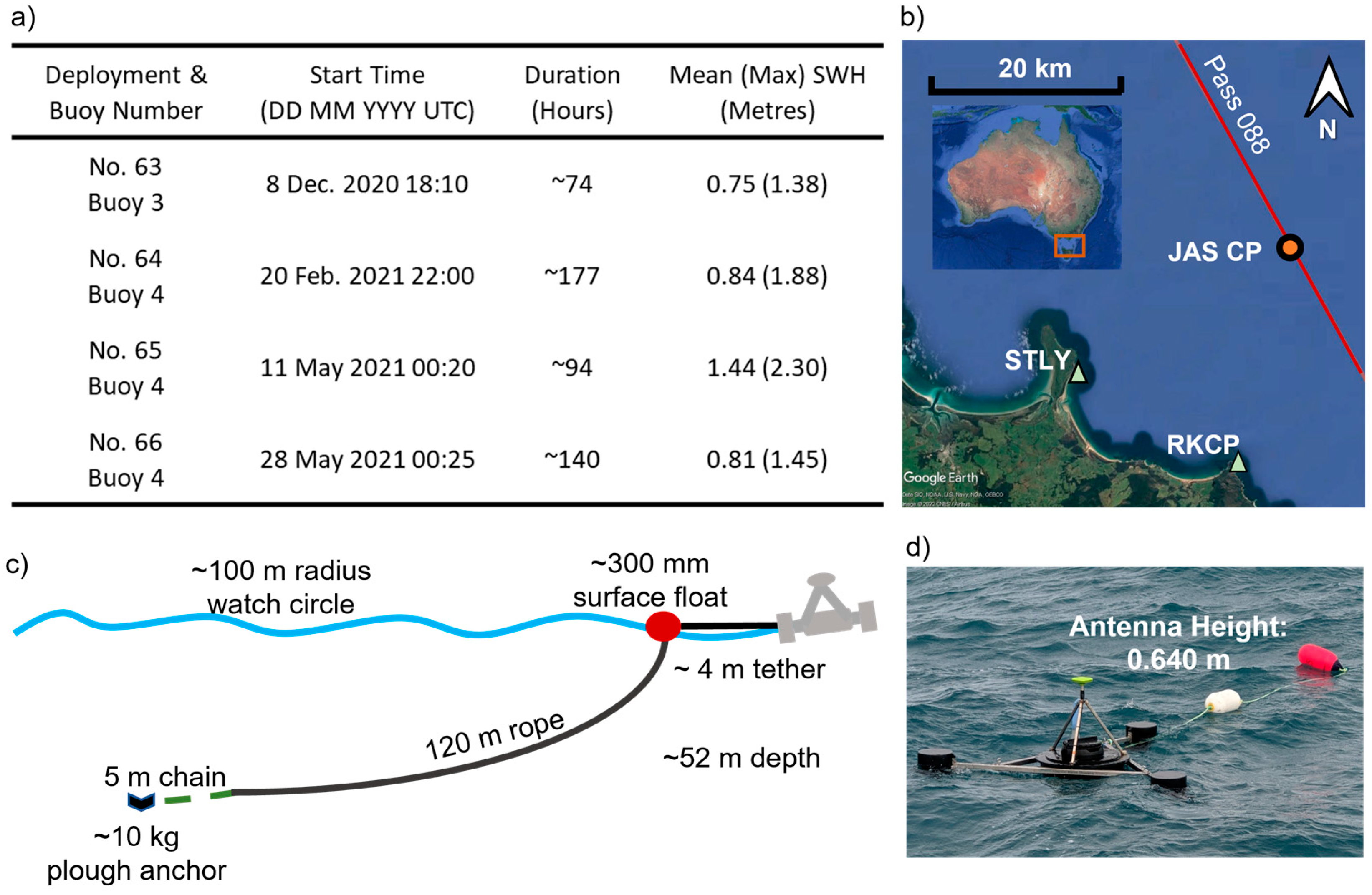
2.1. GNSS/INS Data
2.2. Mooring Data
2.3. ACCESS-G Wind Stress
3. Methods
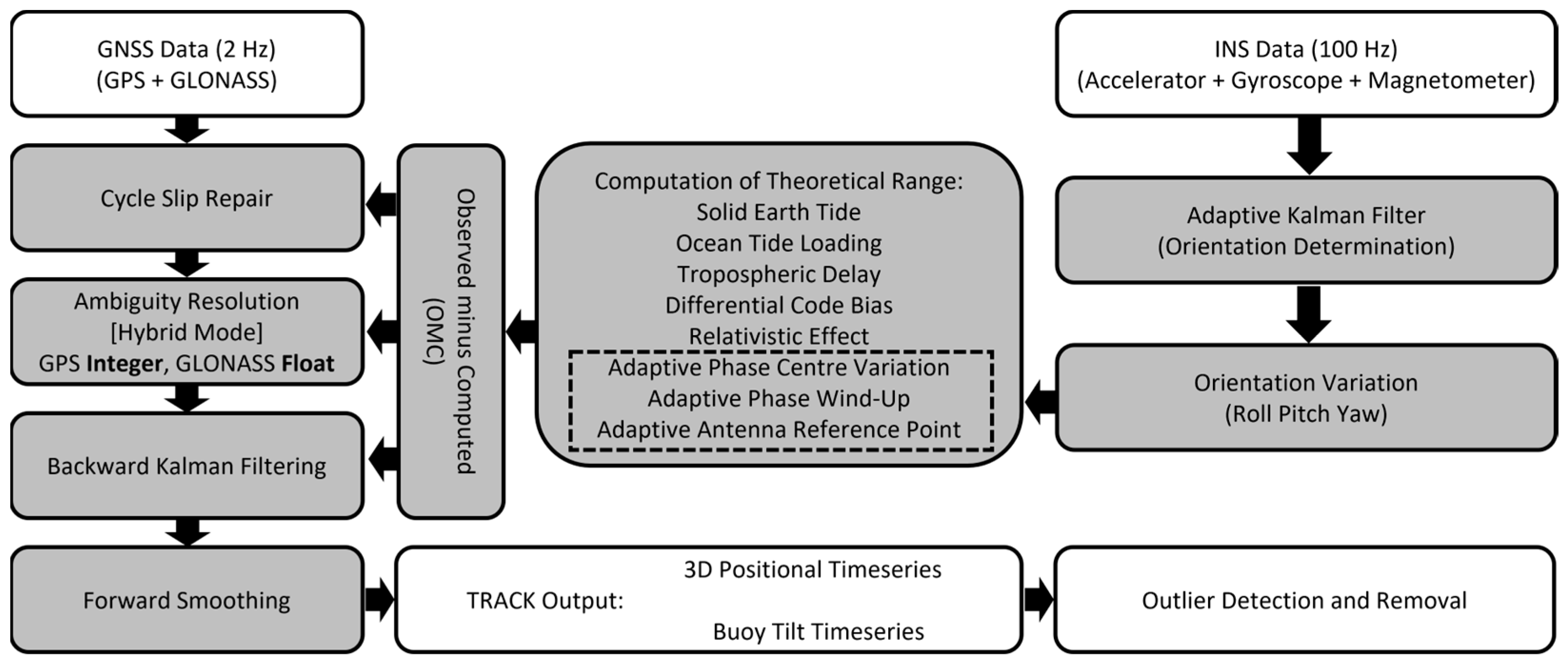
3.1. Processing of GNSS/INS Observations
3.1.1. GNSS Ambiguity Resolution
3.1.2. Outlier Detection and Removal
3.2. Characterising Buoy Dynamics
3.2.1. Vertical Acceleration of the Buoy
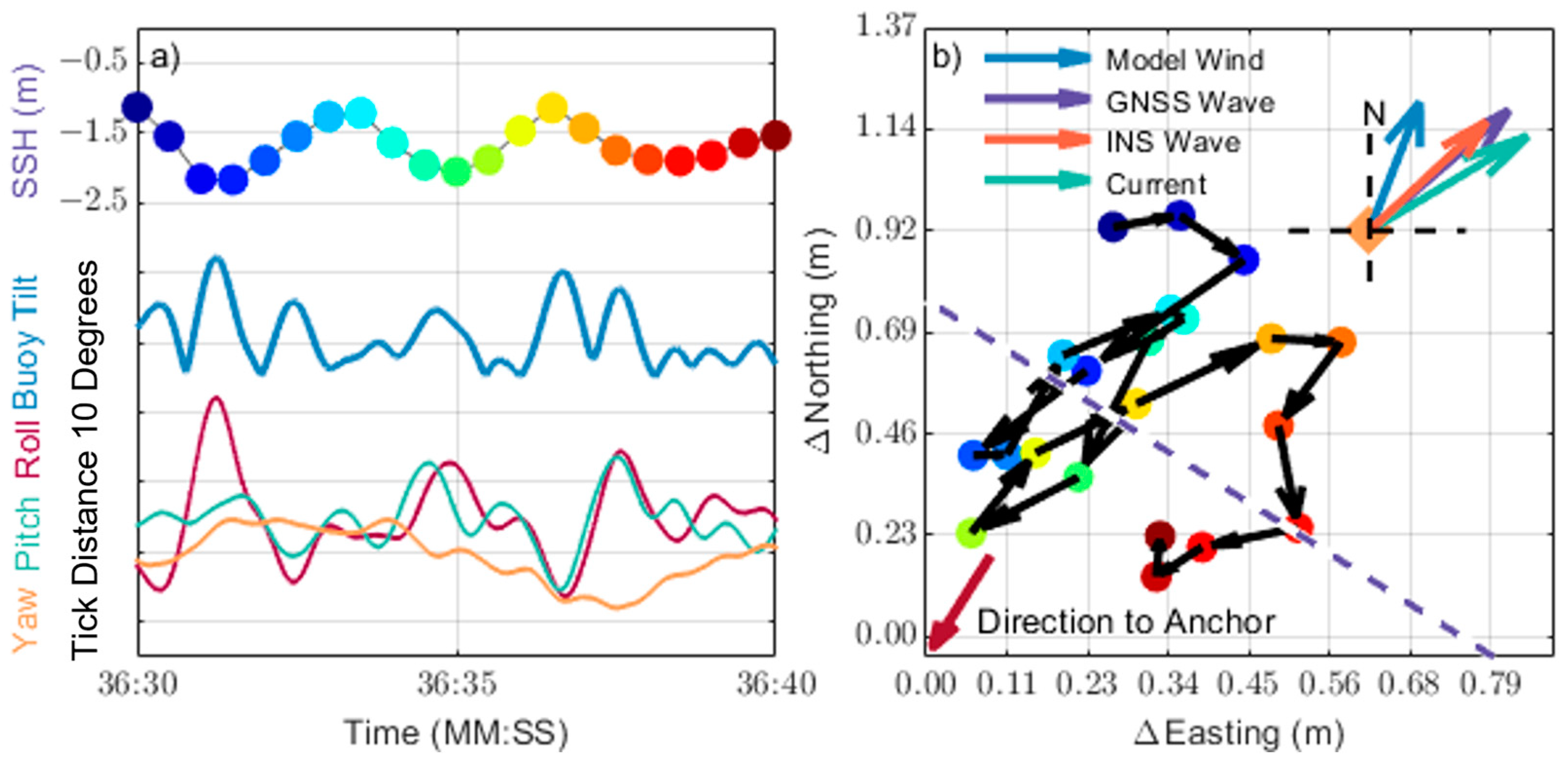
3.2.2. Wave Direction Information as Sensed by the Tethered Buoy
3.2.3. Wave Magnitude Based on SSH Spectrum Analysis
4. Results
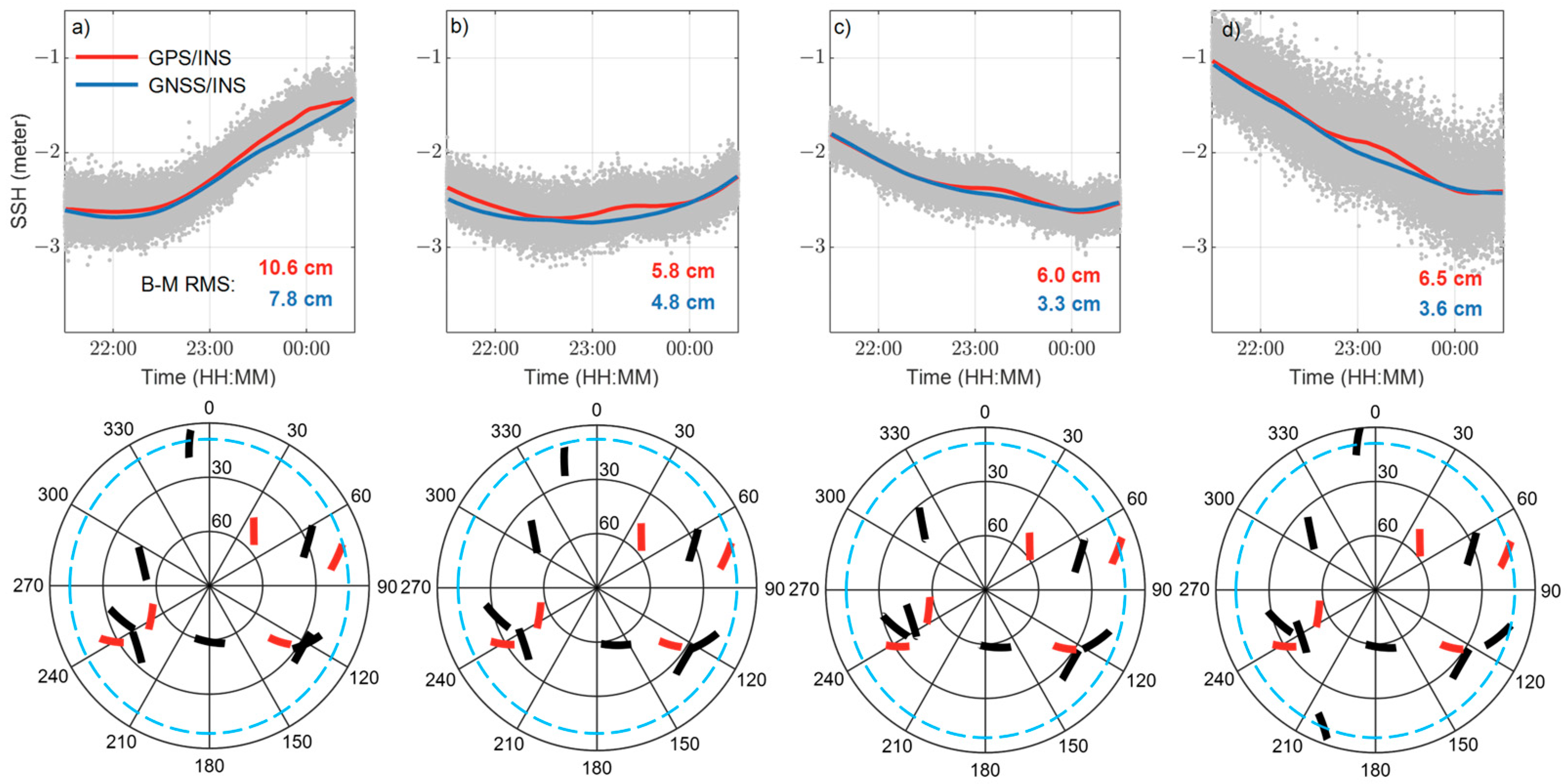
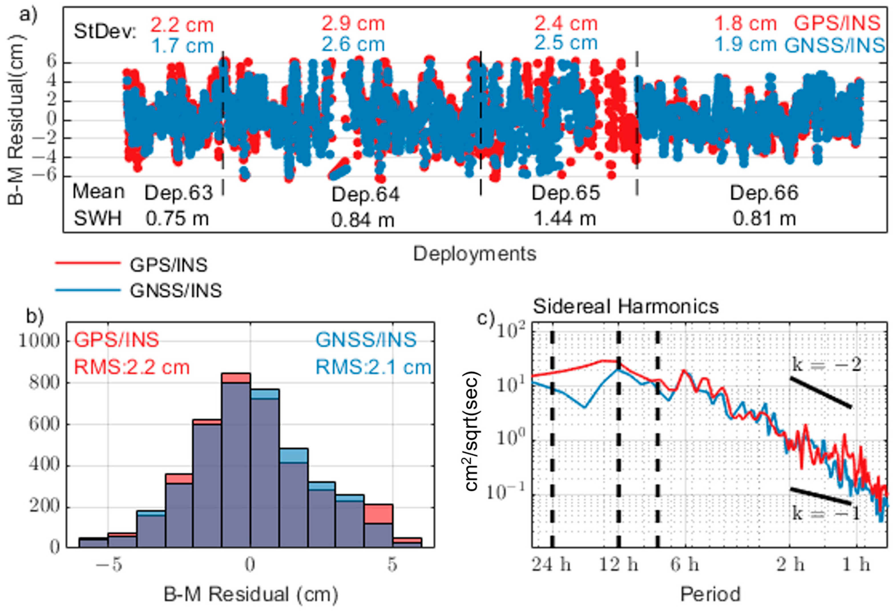
4.1. GPS/INS versus GNSS/INS Buoy Solution—AR Update
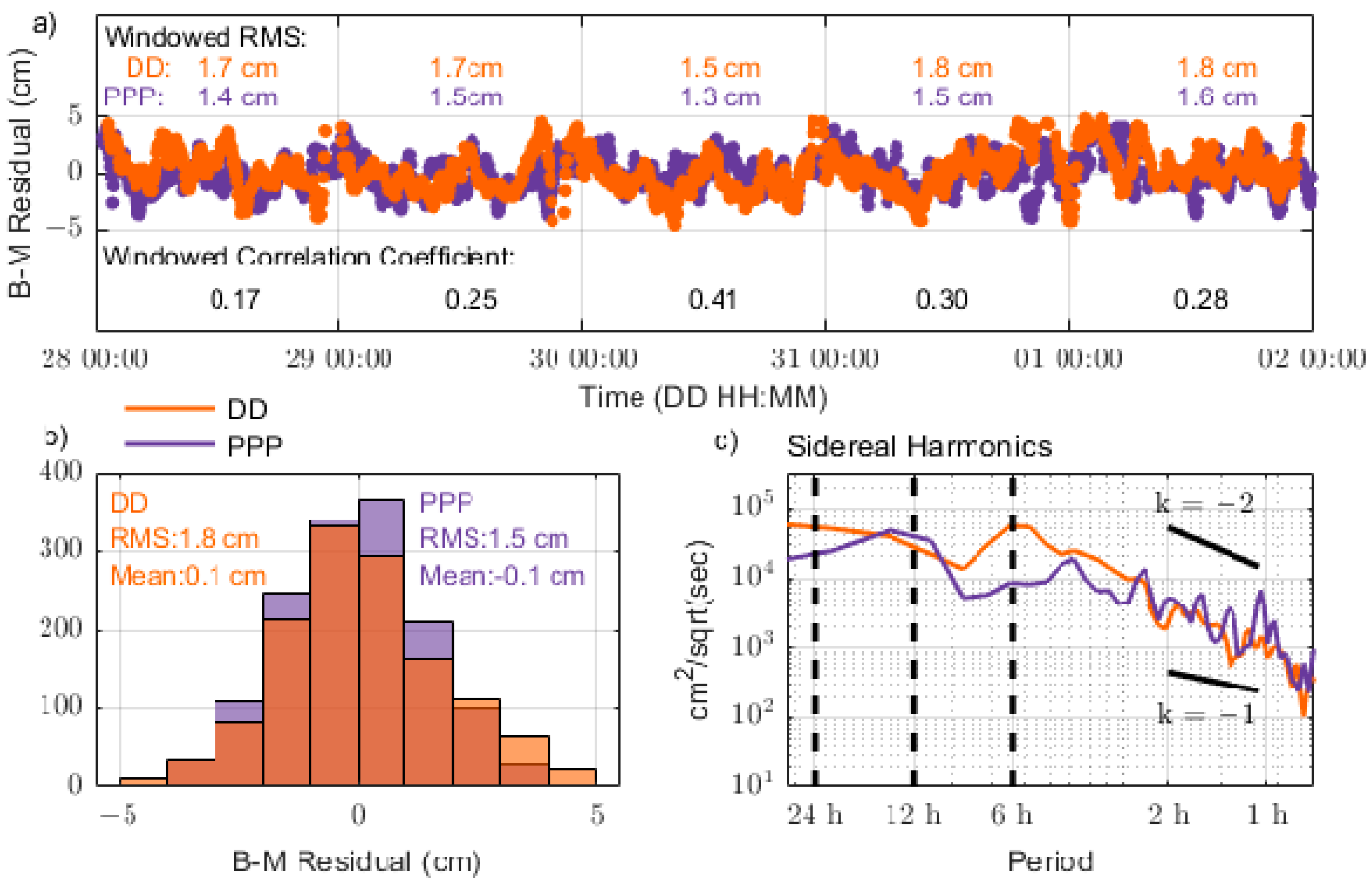
4.2. DD versus PPP Buoy Solution
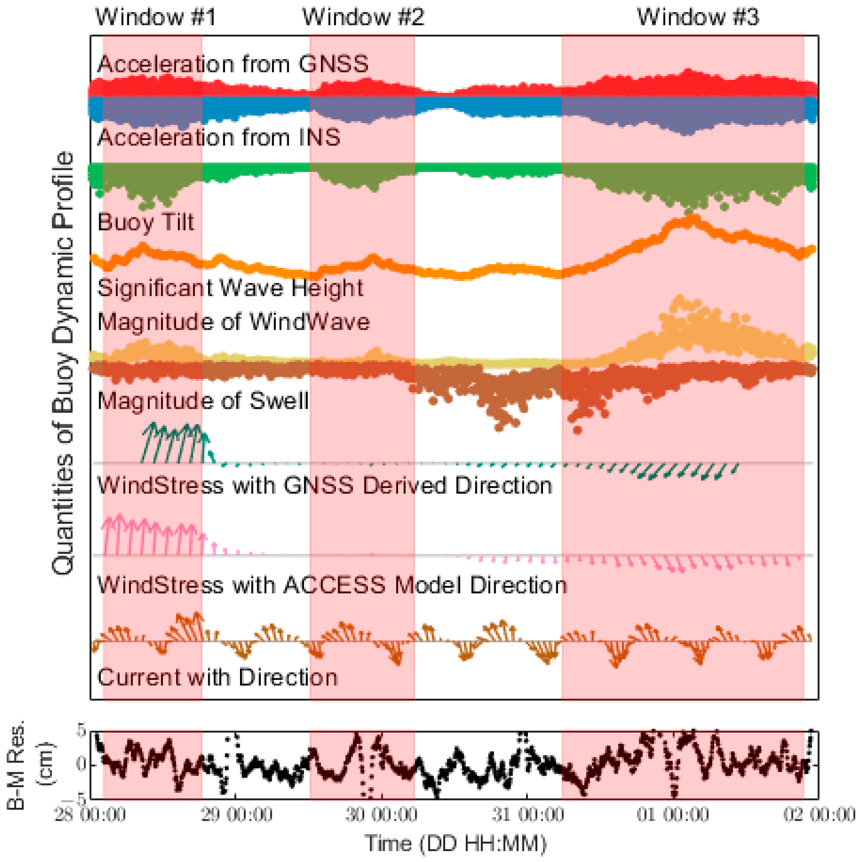
4.3. Measured Indicators of the Buoy Dynamics
4.4. Bias Identification by the Buoy Dynamics
5. Discussion
5.1. Addition of GLONASS
5.2. Processing Strategy
5.3. Contribution of the Buoyancy Variation Due to Dynamics
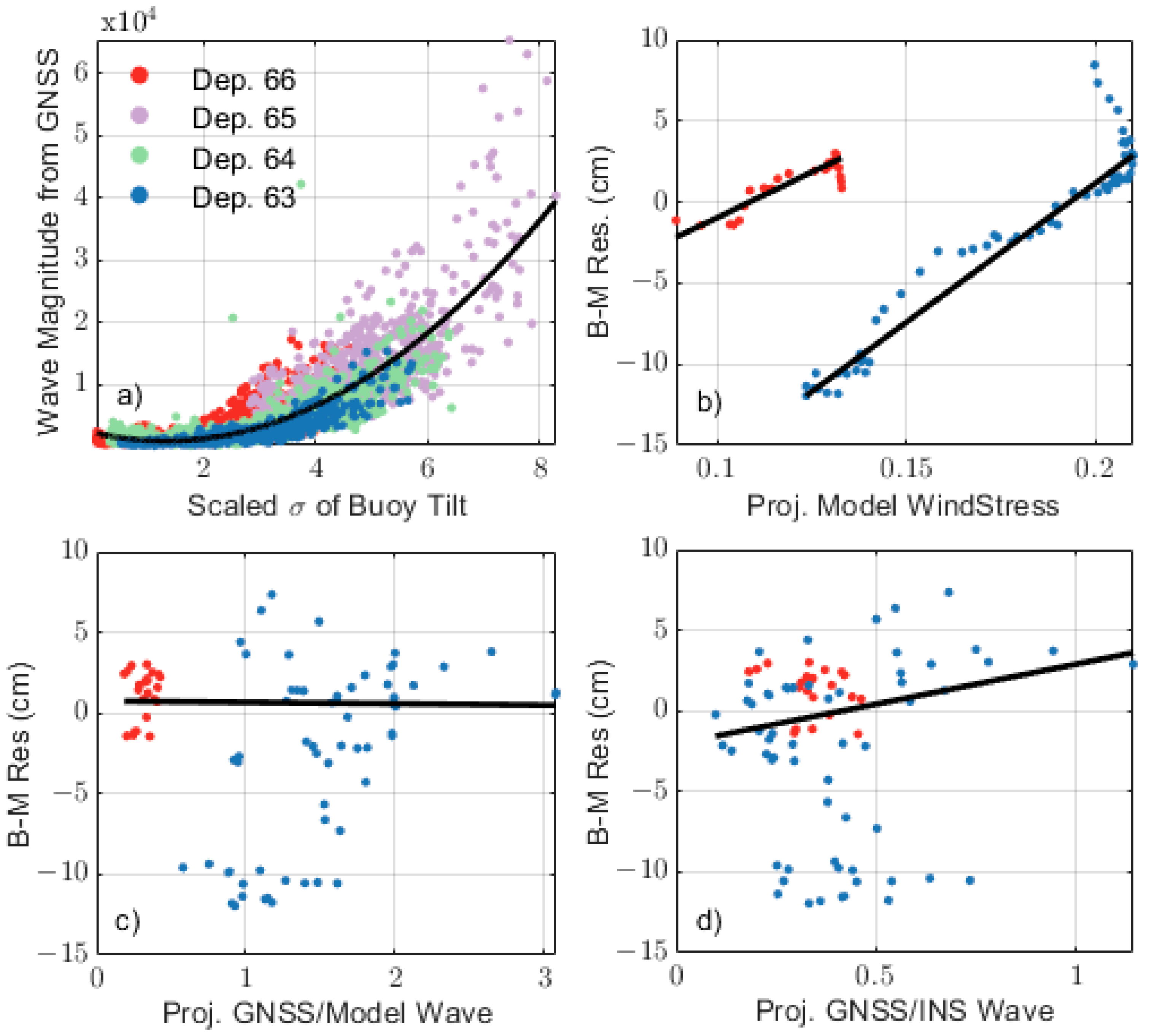
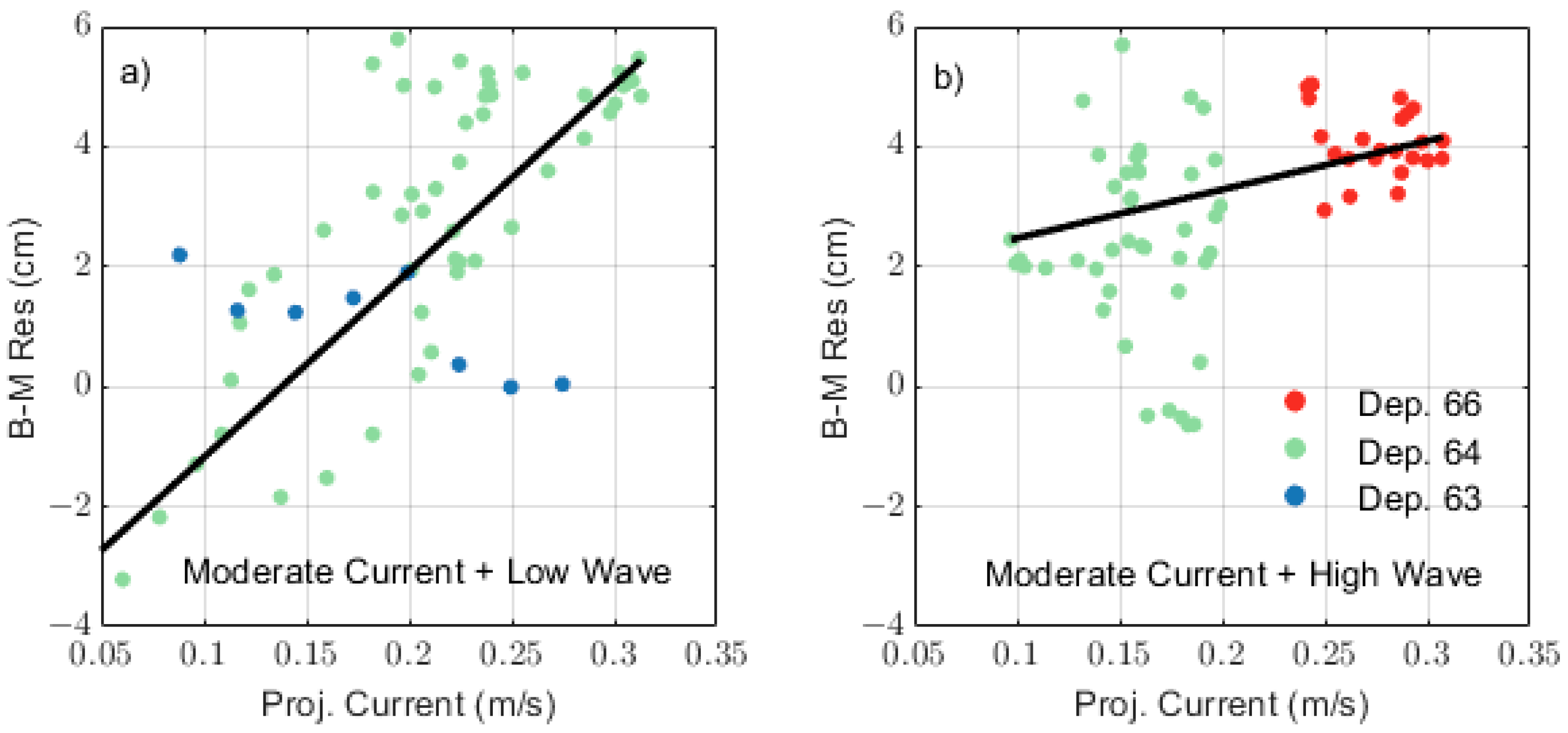
5.4. Relation between Dynamic Indicators and B–M Residuals
5.5. Implication for High-Resolution Altimetry Validation
6. Conclusions
Supplementary Materials
Author Contributions
Funding
Data Availability Statement
Acknowledgments
Conflicts of Interest
References
- Ray, R.D. A Global Ocean Tide Model from TOPEX/POSEIDON Altimetry: GOT99. 2; National Aeronautics and Space Administration, Goddard Space Flight Center: Greenbelt, MD, USA, 1999.
- Fu, L.-L. Ocean circulation and variability from satellite altimetry. In International Geophysics; Elsevier: Amsterdam, The Netherlands, 2001; Volume 77, pp. 141–XXVIII. [Google Scholar]
- Chaigneau, A.; Eldin, G.; Dewitte, B. Eddy activity in the four major upwelling systems from satellite altimetry (1992–2007). Prog. Oceanogr. 2009, 83, 117–123. [Google Scholar] [CrossRef]
- Fu, L.-L.; Chelton, D.B.; Le Traon, P.-Y.; Morrow, R. Eddy dynamics from satellite altimetry. Oceanography 2010, 23, 14–25. [Google Scholar] [CrossRef] [Green Version]
- Desai, S.; Wahr, J.; Beckley, B. Revisiting the pole tide for and from satellite altimetry. J. Geodesy 2015, 89, 1233–1243. [Google Scholar] [CrossRef]
- Faghmous, J.H.; Frenger, I.; Yao, Y.; Warmka, R.; Lindell, A.; Kumar, V. A daily global mesoscale ocean eddy dataset from satellite altimetry. Sci. Data 2015, 2, 1–16. [Google Scholar] [CrossRef] [Green Version]
- Dumont, J.; Rosmorduc, V.; Carrere, L.; Picot, N.; Bronner, E.; Couhert, A.; Guillot, A.; Desai, S.; Bonekamp, H.; Figa, J. Jason-3 Products Handbook; Technical Representative, CNES and EUMETSAT and JPL and NOAA/NESDIS; The National Centre for Space Studies (CNES): Ramonville-St-Agne, France, 2016. [Google Scholar]
- Fernández, J.; Fernández, C.; Féménias, P.; Peter, H. (Eds.) The copernicus sentinel-3 mission. In ILRS Workshop; The International Laser Ranging Service (ILRS): Postdam, Germany, 2016. [Google Scholar]
- Donlon, C.J.; Cullen, R.; Giulicchi, L.; Vuilleumier, P.; Francis, C.R.; Kuschnerus, M.; Simpson, W.; Bouridah, A.; Caleno, M.; Bertoni, R. The Copernicus Sentinel-6 mission: Enhanced continuity of satellite sea level measurements from space. Remote Sens. Environ. 2021, 258, 112395. [Google Scholar] [CrossRef]
- Quartly, G.D.; Nencioli, F.; Raynal, M.; Bonnefond, P.; Nilo Garcia, P.; Garcia-Mondéjar, A.; Flores de la Cruz, A.; Crétaux, J.-F.; Taburet, N.; Frery, M.-L. The roles of the S3MPC: Monitoring, validation and evolution of Sentinel-3 altimetry observations. Remote Sens. 2020, 12, 1763. [Google Scholar] [CrossRef]
- Fernandez, D.E.; Fu, L.L.; Pollard, B.; Vaze, P.; Abelson, R.; Steunou, N. SWOT Project Mission Performance and Error Budget; JPL D-79084; The National Aeronautics and Space Administration: Pasadena, CA, USA, 2017.
- Bonnefond, P.; Exertier, P.; Laurain, O.; Ménard, Y.; Orsoni, A.; Jeansou, E.; Haines, B.J.; Kubitschek, D.G.; Born, G. Leveling the sea surface using a GPS-catamaran special issue: Jason-1 calibration/validation. Mar. Geod. 2003, 26, 319–334. [Google Scholar] [CrossRef]
- Watson, C.; Coleman, R.; White, N.; Church, J.; Govind, R. Absolute calibration of TOPEX/Poseidon and Jason-1 using GPS buoys in bass strait, Australia special issue: Jason-1 calibration/validation. Mar. Geod. 2003, 26, 285–304. [Google Scholar] [CrossRef]
- Penna, N.T.; Morales Maqueda, M.A.; Martin, I.; Guo, J.; Foden, P.R. Sea surface height measurement using a GNSS Wave Glider. Geophys Res. Lett. 2018, 45, 5609–5616. [Google Scholar] [CrossRef]
- Chen, C.; Zhu, J.; Zhai, W.; Yan, L.; Zhao, Y.; Huang, X.; Yang, W. Absolute calibration of HY-2A and Jason-2 altimeters for sea surface height using GPS buoy in Qinglan, China. J. Oceanol. Limnol. 2019, 37, 1533–1541. [Google Scholar] [CrossRef]
- Chupin, C.; Ballu, V.; Testut, L.; Tranchant, Y.-T.; Calzas, M.; Poirier, E.; Coulombier, T.; Laurain, O.; Bonnefond, P.; Project, T.F. Mapping sea surface height using new concepts of kinematic GNSS instruments. Remote Sens. 2020, 12, 2656. [Google Scholar] [CrossRef]
- Zhou, B.; Watson, C.; Legresy, B.; King, M.A.; Beardsley, J.; Deane, A. GNSS/INS-equipped buoys for altimetry validation: Lessons learnt and new directions from the Bass Strait Validation Facility. Remote Sens. 2020, 12, 3001. [Google Scholar] [CrossRef]
- Bonnefond, P.; Haines, B.; Watson, C. In situ absolute calibration and validation: A link from coastal to open-ocean altimetry. In Coastal Altimetry; Springer: Berlin/Heidelberg, Germany, 2011; pp. 259–296. [Google Scholar]
- White, N.J.; Coleman, R.; Church, J.A.; Morgan, P.; Walker, S. A southern hemisphere verification for the TOPEX/POSEIDON satellite altimeter mission. J. Geophys. Res. Ocean. 1994, 99, 24505–24516. [Google Scholar] [CrossRef]
- Watson, C.; White, N.; Church, J.; Burgette, R.; Tregoning, P.; Coleman, R. Absolute calibration in bass strait, Australia: TOPEX, Jason-1 and OSTM/Jason-2. Mar. Geod. 2011, 34, 242–260. [Google Scholar] [CrossRef]
- TRACK MIT. GPS Differential Phase Kinematic Positioning Program. 2011. Available online: geoweb.mit.edu/gg (accessed on 4 January 2021).
- Chen, G. GPS Kinematic Positioning for the Airborne Laser Altimetry at Long Valley, California. Ph.D. Thesis, Massachusetts Institute of Technology, Cambridge, MA, USA, 1998. Available online: https://dspace.mit.edu/handle/1721.1/9680 (accessed on 20 July 2018).
- Lichten, S. GIPSY-OASIS II: A High Precision GPS Data Processing System and General Satellite Orbit. 1995. Available online: hdl.handle.net/2014/31777 (accessed on 7 November 2022).
- Cai, C.; Gao, Y. Modeling and assessment of combined GPS/GLONASS precise point positioning. Gps. Solut. 2013, 17, 223–236. [Google Scholar] [CrossRef]
- Li, X.; Zhang, X.; Guo, F. Study on Precise Point Positioning based on combined GPS and GLONASS. In Proceedings of the 22nd International Technical Meeting of the Satellite Division of the Institute of Navigation (ION GNSS 2009), Savannah, GA, USA, 22–25 September 2009; pp. 2449–2459. [Google Scholar]
- Ge, Y.; Zhou, F.; Sun, B.; Wang, S.; Shi, B. The impact of satellite time group delay and inter-frequency differential code bias corrections on multi-GNSS combined positioning. Sensors 2017, 17, 602. [Google Scholar] [CrossRef] [Green Version]
- Liu, H.; Shu, B.; Xu, L.; Qian, C.; Zhang, R.; Zhang, M. Accounting for inter-system bias in DGNSS positioning with GPS/GLONASS/BDS/Galileo. J. Navig. 2017, 70, 686–698. [Google Scholar] [CrossRef]
- Gao, W.; Pan, S.; Gao, C.; Wang, Q.; Shang, R. Tightly combined GPS and GLONASS for RTK positioning with consideration of differential inter-system phase bias. Meas. Sci. Technol. 2019, 30, 054001. [Google Scholar] [CrossRef]
- Wanninger, L. Carrier-phase inter-frequency biases of GLONASS receivers. J. Geod. 2012, 86, 139–148. [Google Scholar] [CrossRef] [Green Version]
- Geng, J.; Zhao, Q.; Shi, C.; Liu, J. A review on the inter-frequency biases of GLONASS carrier-phase data. J. Geod. 2017, 91, 329–340. [Google Scholar] [CrossRef]
- Cherneva, Z.; Andreeva, N.; Pilar, P.; Valchev, N.; Petrova, P.; Soares, C.G. Validation of the WAMC4 wave model for the Black Sea. Coast Eng. 2008, 55, 881–893. [Google Scholar] [CrossRef]
- Akpınar, A.; van Vledder, G.P.; Kömürcü, M.İ.; Özger, M. Evaluation of the numerical wave model (SWAN) for wave simulation in the Black Sea. Cont. Shelf Res. 2012, 50, 80–99. [Google Scholar] [CrossRef]
- Wang, S.; Liu, L.; Jin, R.; Chen, S. Wave Height Measuring Device Based on Gyroscope and Accelerometer. In Proceedings of the 2019 IEEE International Conference on Mechatronics and Automation (ICMA), Tianjin, China, 4–7 August 2019; pp. 701–706. [Google Scholar]
- Welch, P. The use of fast Fourier transform for the estimation of power spectra: A method based on time averaging over short, modified periodograms. IEEE Trans. Audio Electroacoust. 1967, 15, 70–73. [Google Scholar] [CrossRef] [Green Version]
- Amiri-Simkooei, A. Noise in multivariate GPS position time-series. J. Geod. 2009, 83, 175–187. [Google Scholar] [CrossRef] [Green Version]
- Geng, J.; Pan, Y.; Li, X.; Guo, J.; Liu, J.; Chen, X.; Zhang, Y. Noise characteristics of high-rate multi-GNSS for subdaily crustal deformation monitoring. J. Geophys. Res. Solid Earth 2018, 123, 1987–2002. [Google Scholar] [CrossRef]
- Kouba, J.; Lahaye, F.; Tétreault, P. Precise point positioning. In Springer Handbook of Global Navigation Satellite Systems; Springer: Berlin/Heidelberg, Germany, 2017; pp. 723–751. [Google Scholar]
- Löfgren, J.S.; Haas, R.; Scherneck, H.-G. Sea level time series and ocean tide analysis from multipath signals at five GPS sites in different parts of the world. J. Geodyn. 2014, 80, 66–80. [Google Scholar] [CrossRef] [Green Version]
- King, M.A.; Watson, C.S. Long GPS coordinate time series: Multipath and geometry effects. J. Geophys. Res. Solid Earth 2010, 115. [Google Scholar] [CrossRef]
- Wielgosz, P.; GREJNER-BRZEZINSKA, D.; Kashani, I. High-Accuracy DGPS and Precise Point Positioning Based on Ohio CORS Network. Navigation 2005, 52, 23–28. [Google Scholar] [CrossRef]
- Xiaohong, Z.; Xingxing, L.; Pan, L. Review of GNSS PPP and its application. Acta Geod. Cartogr. Sin. 2017, 46, 1399. [Google Scholar]
- Fund, F.; Perosanz, F.; Testut, L.; Loyer, S. An Integer Precise Point Positioning technique for sea surface observations using a GPS buoy. Adv. Space Res. 2013, 51, 1311–1322. [Google Scholar] [CrossRef]


Disclaimer/Publisher’s Note: The statements, opinions and data contained in all publications are solely those of the individual author(s) and contributor(s) and not of MDPI and/or the editor(s). MDPI and/or the editor(s) disclaim responsibility for any injury to people or property resulting from any ideas, methods, instructions or products referred to in the content. |
© 2023 by the authors. Licensee MDPI, Basel, Switzerland. This article is an open access article distributed under the terms and conditions of the Creative Commons Attribution (CC BY) license (https://creativecommons.org/licenses/by/4.0/).
Share and Cite
Zhou, B.; Watson, C.; Legresy, B.; King, M.A.; Beardsley, J. Ongoing Development of the Bass Strait GNSS/INS Buoy System for Altimetry Validation in Preparation for SWOT. Remote Sens. 2023, 15, 287. https://doi.org/10.3390/rs15010287
Zhou B, Watson C, Legresy B, King MA, Beardsley J. Ongoing Development of the Bass Strait GNSS/INS Buoy System for Altimetry Validation in Preparation for SWOT. Remote Sensing. 2023; 15(1):287. https://doi.org/10.3390/rs15010287
Chicago/Turabian StyleZhou, Boye, Christopher Watson, Benoit Legresy, Matt A. King, and Jack Beardsley. 2023. "Ongoing Development of the Bass Strait GNSS/INS Buoy System for Altimetry Validation in Preparation for SWOT" Remote Sensing 15, no. 1: 287. https://doi.org/10.3390/rs15010287