Evaluation of Sentinel-6 Altimetry Data over Ocean

Abstract

The Sentinel-6 Michael Freilich (S6-MF) satellite was launched on 21st November 2020. Poseidon-4, the main payload onboard S6-MF, is the first synthetic aperture radar (SAR) altimeter operating in an interleaved open burst mode. In this study, the sea surface height (SSH), significant wave height (SWH) and wind speed observations from the Poseidon-4 Level 2 altimetry products from November 2021 to October 2022 are assessed. The assessment contains synthetic aperture radar mode (SARM) as well as low-resolution mode (LRM) data. The SSH assessment is conducted using range noise, sea level anomaly (SLA) spectral analysis and crossover analysis, whereas the SWH and wind speed assessments are performed against NDBC buoy data and other satellite altimetry missions. The performance of the Sentinel-6 altimetry data is compared to those of Sentinel-3A/B and Jason-3 altimetry data. The 20 Hz range noise is 3.07 cm for SARM and 6.40 cm for LRM when SWH is 2 m. The standard deviation (STD) of SSH differences at crossovers is 3.76 cm for SARM and 4.27 cm for LRM. Compared against the NDBC measurements, the Sentinel-6 SWH measurements have a root-mean-square error (RMSE) of 0.361 m for SARM and an RMSE of 0.225 m for LRM. The Sentinel-6 wind speed measurements show an RMSE of 1.216 m/s for SARM and an RMSE of 1.323 m/s for LRM. We also present the impacts of ocean waves on parameter retrievals from Sentinel-6 SARM data. The Sentinel-6 SARM data are sensitive to wave period and direction as well as vertical velocity. It should be paid attention to in the future.

1. Introduction

A radar altimeter is able to measure the SSH, SWH and wind speed by transmitting electromagnetic waves and receiving echoes returned from the surface. The data measured by the radar altimeter can be further used for study of global and regional sea level variation [1,2], marine gravity anomalies [3], geoids [4], seafloor topography [5], ocean tides [6], wind–wave fields [7] and ocean dynamics [8]. With the development of technology, radar altimeter data can be used not only for oceanographic research but also for inland water level changes [9,10,11], sea ice thickness and volume changes [12,13,14] and ice sheet mass balance [15,16,17].

The spatial resolution of the conventional pulse-limited radar altimeter, such as the altimeters onboard Jason-1/2/3 satellites, is limited by the radar altimeter’s pulse-limited footprint. The pulse-limited footprint is approximately 2 km in diameter, and it can increase to several kilometers as SWH increases. The SAR altimeter or delay/Doppler radar altimeter has better along-track resolution and precision than the conventional pulse-limited altimeters [18]. The along-track footprint size of the SAR altimeter is reduced to approximately 300 m and does not vary with SWH [19]. Furthermore, the speckle noise is also reduced because of more independent looks to be averaged. The radar altimeter onboard the CryoSat-2 satellite first used SARM over sea ice and a few oceanic regions. Due to SARM’s high performance over open ocean [13,20], the radar altimeters for the Sentinel-3 mission operate in SARM globally. The CryoSat-2 and Sentinel-3 SARM data have been widely used for research over ocean [20,21], sea ice [22], ice sheets [23] and inland [24].

The SAR altimeters for CryoSat-2 and Sentinel-3 missions use a closed burst mode. The radar altimeters transmit bursts composed of 64 pulses and group the received data from a continuous PRF (around 18 kHz) into consecutive sets each of 64 pulses [25,26]. The duration of each burst is about 3.5 ms and the burst repetition interval is about 11.8 ms. Therefore, more than half of the opportunity to make measurements is unused. To avoid the defects of the closed burst SAR mode, the SAR altimeter onboard the Sentinel-6 satellite operates in an interleaved open-burst mode and its PRF is around 9 kHz. The transmitting and receiving pulses are alternately carried out. Interleaved mode could lead to more independent looks and allow SAR and pulse limited data to be gathered simultaneously [27].

Copernicus Sentinel-6 is the new altimetry reference mission to provide global sea level measurements. The Sentinel-6 mission has two satellites. The first one is S6-MF and the second is scheduled to be launched in 2025. Poseidon-4, which is designed to provide SSH, SWH and wind speed data with high precision, is the primary payload of S6-MF. It is the first SAR altimeter that operates in an interleaved open-burst mode.

The Poseidon-4 Level 2 altimetry products are assessed in this study. The SSH assessment is conducted using range noise, SLA spectral analysis and crossover analysis, whereas the SWH and wind speed assessments are performed against NDBC buoy data and other satellite altimetry data. We also present the impacts of ocean waves on range, SWH and sigma0 retrievals from Sentinel-6 altimetry data using the several wave parameters derived from ERA5 re-analysis data.

2. Materials and Methods

2.1. NDBC SWH and Wind Speed Data

The National Data Buoy Center (NDBC) buoy data are applied to evaluate and validate the Sentinel-6 altimeter derived SWH and wind speed. The NDBC SWH and wind speed measurements are available hourly [28,29]. We only used buoys that are more than 50 km from the shoreline to avoid the influence of land. Figure 1 shows the locations of the 78 buoys used in this study. The height of the wind speed measurements by the NDBC buoys is 4 m above the sea surface. However, the wind speed estimated by the altimeter is on a level of 10 m above the surface. For direct comparison of the altimeter and buoy data, the NDBC buoy wind speeds were converted to speeds at 10 m above the sea surface using the methods presented in Durden et al. [30].

2.2. ERA5 Re-analysis Data

ERA5 is the latest global re-analysis data set launched by the European Centre for Medium-Range Weather Forecasts (ECMWF). ERA5 provides the re-analysis data from 1979 to the present and is still being updated. Any user can obtain the ERA5 re-analysis data for free. ERA5 is the successor of ERA-Interim re-analysis [31]. Compared with ERA-Interim, ERA5 has been greatly improved. ERA-Interim’s spatial resolution and temporal resolution are 0.75° and 6 h, respectively. The spatial resolution and temporal resolution of ERA5 are, respectively, 0.25° and 1 h, which are much higher than those of ERA-Interim.

In this study, we aimed to investigate the impacts of ocean waves on range, SWH and sigma0 retrievals from Sentinel-6 altimetry data. The mean zero-crossing wave period (T02), mean wave direction (MWD) and significant height of combined wind waves and swell (SWH) from ERA5 re-analysis are used in this study.

2.3. Satellite Altimetry Data

Sentinel-3A/B and Jason-3 altimetry data were also used to assess and validate the Sentinel-6 altimetry data.

Table 1. Information of the satellite altimetry data used.

Satellite	Inclination (°)	Repeat Period (days)	Data Type	Radar Mode	Source
Sentinel-6	66.0	9.9	L2 NTC	SAR (Open Burst) /LRM	EUMETSAT
Sentinel-3A	98.6	27	L2 NTC	SAR (Closed Burst)	EUMETSAT
Sentinel-3B	98.6	27	L2 NTC	SAR (Closed Burst)	EUMETSAT
Jason-3	66.0	9.9	GDR-F	LRM	AVISO

gives the information of the altimetry data we used.

2.3.1. Sentinel-6 Altimetry Data

Sentinel-6 is a non-Sun-synchronous satellite. Its mean altitude and inclination are 1336 km and 66°, respectively. Poseidon-4 is the main payload of Sentinel-6 and is a SAR altimeter operating at the Ku-band and C-band. The C-band measurements are mainly used for ionospheric corrections. Poseidon-4 can provide measurements of SSH, SWH and wind speed. Poseidon-4 uses an interleaved open burst. More independent looks are obtained compared to the Sentinel-3A/B SAR altimeter and it can reduce the altimeter’s instrument noise.

There are three types of Poseidon-4 L2 products available: near real time (NRT), short time critical (STC) and non-time critical (NTC) products. The disseminations of the NRT, STC and NTC products are respectively due within 2 h, 36 h and 60 days after data acquisition. The Poseidon-4 L2 products contain the geophysical information derived from the altimeter: range, orbital altitude, time, range and geophysical corrections, SWH and wind speed. In this study, we evaluated the Poseidon-4 NTC Level 2 altimetry products from November 2021 to October 2022, focusing on the SSH, SWH and wind speed. Our assessment involves both LRM and SARM data.

2.3.2. Sentinel-3A/B Altimetry Data

Sentinel-3A, launched on 16 February 2016 and Sentinel-3B, launched on 25 April 2018 make up the Sentinel-3 mission. The mean altitude and inclination for Sentinel-3A/B are 815 km and 98.6°, respectively. The repeat cycle of Sentinel-3A/3B is 27 days. The SAR altimeter (SARL) onboard Sentinel-3A/B uses a closed burst. SARL is inherited from the CryoSat-2 radar altimeter.

The SARL NRT, STC and NTC L2 products are available. We used the NTC L2 data downloaded from the EUMETSAT Data Centre. The NTC L2 products contain three data files: “reduced”, “standard” and “enhanced” data files. We used the “enhanced” data in this study. The SARL NTC L2 enhanced products provide 1 Hz measurements as well as 20 Hz measurements.

2.3.3. Jason-3 Altimetry Data

Jason-3, launched on 17 January 2016, is an altimetry reference mission designed to succeed Topex/Poseidon, Jason-1 and Jason-2. These altimetry missions provide sea level measurements from 1992 to the present. Jason-3 is a non-Sun-synchronous satellite. Its mean altitude and inclination are 1336 km and 66°, respectively. The repeat cycle of Jason-3 is 9.9156 days. The radar altimeter onboard Jason-3 is a pulse-limited altimeter that operates in low-resolution mode (LRM).

The latest version of the Jason-3 Geophysical Data Records (GDR-F) data is used in this study. Similar to the Sentinel-3A/B NTC L2 products, the GDR-F products provide both 1 Hz and 20 Hz measurements. Adaptive re-tracking is first used in Jason-3 GDR-F products. The adaptive re-tracking fit from a Brown numerical model takes the real onboard PTR while MLE4 and MLE3 re-tracking used in the Jason-3 GDR-E product fit are taken from a 2nd order Brown analytical model [32]. Besides the adaptive re-tracking, the Jason-3 GDR-F products also contain results from MLE4 and MLE3 re-tracking.

2.4. Data Analysis Methods

The 20 Hz measurement noise is computed as the STD of the valid measurements in a 20 Hz data block. It has been widely applied to satellite altimetry assessments as a standard measure of the precision of the observed parameters [27,33]. In this study, we computed the measurement noise of range, SWH and sigma0 measurements. In addition, the SLA power spectral density (PSD) was computed using the along-track SLA measurements using the periodogram method and the SLA noise was derived from the SLA PSD.

To evaluate the accuracy of the SSH measurements derived from Sentinel-6, we computed the mean and STD of the SSH differences at mono-mission crossovers. The multi-mission cross-calibration assessment was also used to evaluate the SSH measurements using Sentinel-3A/B and Jason-3 altimetry data.

The altimeter-derived SWH and wind speed measurements are generally validated by a comparison against NDBC data. The altimeter and NDBC buoy data should first be collocated. There are many collocation methods that have been used for SWH and wind speed validation. We only selected the altimeter data that are less than 50 km from the buoy position, and their mean value is taken as satellite altimeter data value. Quality control should be conducted before averaging. NDBC SWH or wind speed measurement values are linearly interpolated to the altimeter measurement time. This interpolated NDBC measurement and the averaged altimeter measurement form a single collocation. We only used the collocations whose time difference is less than 0.5 h.

The statistical parameters used in this study are the bias, STD, RMSE and correlation coefficient (R) [34]:

$$Bias=\frac{1}{N}{\displaystyle \sum _{i=1}^N(S_i-B_i)}$$

(1)

$$STD=\sqrt{\frac{{{\displaystyle \sum _{i=1}^N(S_i-B_i-\overline{S-B})}}^2}{N-1}}$$

(2)

$$RMSE=\sqrt{\frac{{{\displaystyle \sum _{i=1}^N(S_i-B_i)}}^2}{N}}$$

(3)

$$R=\frac{{\displaystyle \sum _{i=1}^N(S_i-\overline{S})}(B_i-\overline{B})}{\sqrt{{{\displaystyle \sum _{i=1}^N(S_i-\overline{S})}}^2{{\displaystyle \sum _{i=1}^N(B_i-\overline{B})}}^2}}$$

(4)

where N is the number of collocations, $B_i$ is the NDBC buoy measurement and $S_i$ is the satellite altimeter measurement. These four statistical parameters are capable of characterizing the error property of the altimeter-derived SWH or wind speed measurements together.

3. Results

3.1. Assessment of Sea Surface Height

3.1.1. Range Noise Analysis

Range is the altimeter-measured distance from the satellite to the sea surface corresponding to the sub-satellite point [35]. The 20 Hz range is obtained by adding the tracking range onboard, the instrument error corrections and the re-tracking correction derived by re-tracking the 20 Hz waveforms. The 1 Hz products are most commonly used in oceanography. Each 1 Hz range is derived from the linear regression of the respective 20 Hz range measurements [35]. The 20 Hz range noise is derived by calculating the STD of the differences between the valid 20 Hz measurements and the derived 1 Hz measurement [27,34,35]. When computing the 20 Hz range noise, the range is not corrected by tropospheric effect, ionospheric effect, sea state bias and tides because their variations within one second are negligible. Assuming that noise in the 20 Hz measurements is independent, the 1 Hz range noise can be estimated by dividing the 20 Hz STD by $\sqrt{N}$, where $N$ is the valid number of the 20 Hz data used to compute the 1 Hz range.

Figure 2 shows the 20 Hz and 1 Hz range noises estimated from several altimetry missions. The Sentinel-6, Sentinel-3A/B and Jason-3 altimetry data from November 2021 to October 2022 (Sentinel-6 Cycle 37 to Cycle 71) over the global ocean were used to calculate the range noise. However, we removed the data at high latitudes (above 50°) to reduce the influence of sea ice. The range noises increase with the increasing of SWH. When SWH increases, the slope of the leading edge of the altimeter waveform decreases, then the precision in the timing of the mid-point of the leading edge is also reduced [33]. The Sentinel-6 SARM has lower 20 Hz range noise than the Sentiel-3A/B and Jason-3 missions. At 2 m SWH, the 20 Hz range noises of the Sentinel-6 SARM and LRM are 3.07 cm and 6.40 cm, respectively. The 20 Hz range noises of the Sentinel-3A (4.88 cm) and Sentinel-3B (4.86 cm) SARM are almost identical. The Jason-3 adaptive re-tracking (6.55 cm) obtains lower noise than the MLE4 re-tracking (7.12 cm). The 20 Hz range noises derived in this study are close to the preliminary range noise estimates derived from Sentinel-6 Poseidon-4 SARM (3.2 cm) and LRM (6.2 cm) data presented in Donlon et al. [27] (SWH = 2 m, sigma0 = 11 dB).

As shown in Figure 2b, the Sentinel-6 SARM data have the lowest 1 Hz range noise among the six data sets. The 1 Hz range noises for Sentinel-6 SARM, Sentinel-6 LRM, Sentinel-3A SARM, Sentinel-3B SARM, Jason-3 MLE and Jason-3 adaptive re-tracking data are, respectively, 0.70 cm, 1.43 cm, 1.09 cm, 1.08 cm, 1.59 cm and 1.46 cm. On the whole, the range noises derived from SARM are lower than those from LRM. However, the range noise of the Sentinel-6 LRM data is lower than those of Sentinel-3A/B SARM data when SWH is above 6 m.

3.1.2. Sea Level Anomaly (SLA) Spectral Analysis

The along-track SLA spectral analysis has been widely used to assess the altimetry mission’s performance [20,33,36,37]. The SSH derived from the altimeter can be expressed as [38]:

$$SSH=H-(R+\Delta R_{corr})$$

(5)

$$\Delta R_{corr}=\Delta R_{dry}+\Delta R_{wet}+\Delta R_{iono}+\Delta R_{ssb}+\Delta R_{ocean}+\Delta R_{solid}+\Delta R_{pole}+\Delta R_{DAC}$$

(6)

where $H$ is the satellite altitude above the reference ellipsoid, $R$ is the altimeter range, $\Delta R_{dry}$ is the dry tropospheric correction, $\Delta R_{wet}$ is the wet tropospheric correction, $\Delta R_{iono}$ is the ionospheric correction, $\Delta R_{ssb}$ is the sea state bias correction, $\Delta R_{ocean}$ is the geocentric ocean tide, $\Delta R_{solid}$ is the solid earth tide, $\Delta R_{pole}$ is the polar tide and $\Delta R_{DAC}$ is the dynamic atmospheric correction. We used the range corrections provided in the altimetry products. Radiometer wet troposphere correction and filtered dual frequency ionospheric correction were used to calculate the SSH measurements.

The SLA is computed by subtracting the mean sea surface (MSS) from the SSH. We used the CNES-CLS15 MSS model data to calculate the SLA measurements for Sentinel-6, Sentinel-3A/B and Jason-3. In this study, we present the SLA PSD for the 20 Hz and 1 Hz SLA measurements. The SLA PSD is computed on a logarithmic frequency scale. The SLA noise is then derived from the SLA PSD using the method presented in Zanifé et al. [39]. The Sentinel-6, Sentinel-3A/B and Jason-3 altimetry data from January 2022 were used to calculate the SLA PSDs at a global scale.

As shown in Figure 3a, there is a spectral hump on the SLA PSDs of the Sentinel-6 LRM and Jason-3 data when the wavelength is between 30 km and 5 km. However, the hump is absent on the SLA PSDs of the Sentinel-6 and Sentinel-3A/B SARM data. The SARM data have much lower SLA noise than the LRM data due to Doppler processing. The 20 Hz SLA noise is 3.86 cm for the Sentinel-6 SARM, 6.97 cm for Sentinel-6 LRM, 5.59 cm for Sentinel-3A SARM, 5.62 cm for Sentinel-3B SARM, 7.94 cm for Jason-3 MLE4 and 7.23 cm for Jason-3 adaptive re-tracking. The SLA PSDs are estimated at a global scale. Therefore, the SLA noise is related to the global mean sea state. The global mean SWH is around 2.5 cm. We can see that the 20 Hz SLA noises are close to the 20 Hz range noises at 2.5 cm derived in Section 3.1.1.

Figure 3b shows the 1 Hz SLA PSDs. The spectral hump is not visible in the 1 Hz data since the sampling rate (6–7 km) is insufficient to sample the relevant wavenumbers. The 1 Hz SLA noise for Sentinel-6 LRM (3.55 cm) is very close to that for Jason-3 MLE4 (3.51 cm) and slightly higher than that for Jason-3 re-tracking (3.37 cm). The 1 Hz SLA noise for Sentinel-6 SARM (2.64 cm) is very close to those for Sentinel-3A SARM (2.63 cm) and Sentinel-3B SARM (2.65 cm). The 1 Hz SLA noise derived from the PSD represents not only Gaussian noise but also a contribution from the spectral hump affecting the PSD of the 20 Hz LRM data [33,37].

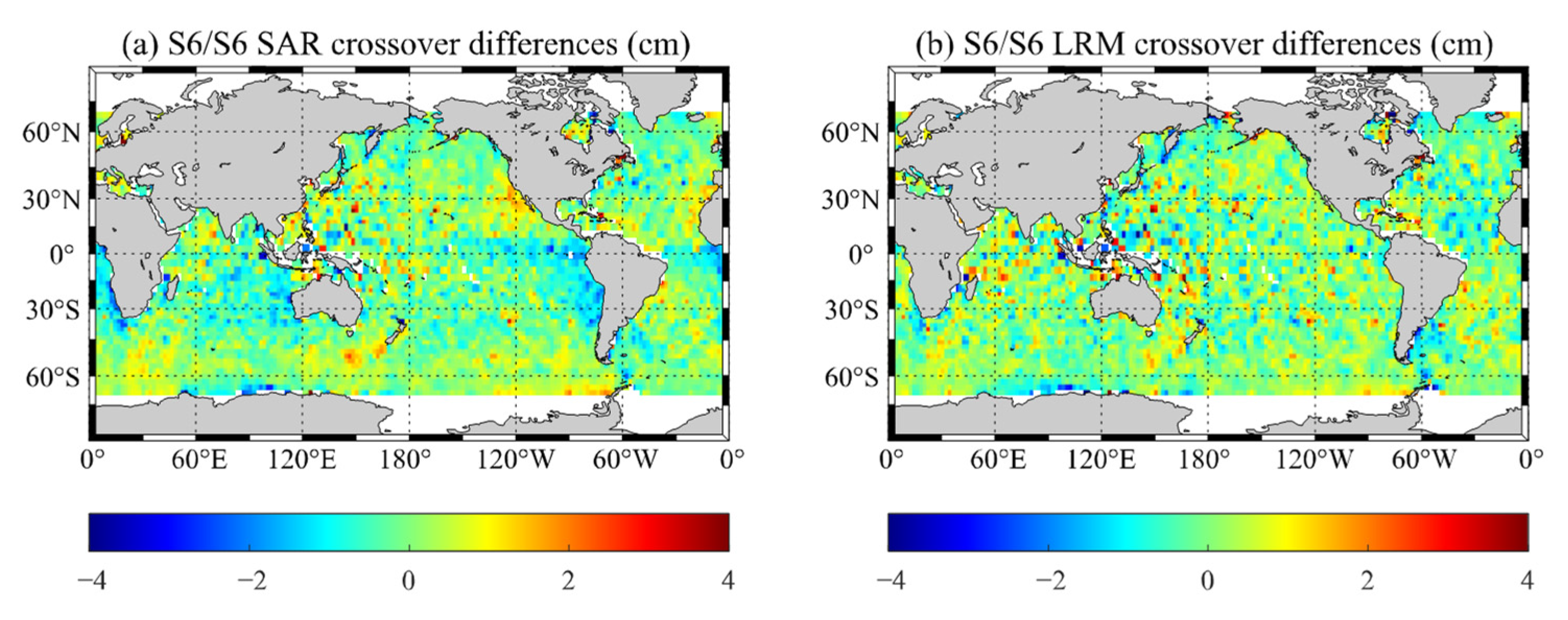
3.1.3. SSH Crossover Analysis

The global SSH crossover analysis is widely applied to evaluate the SSH measurements derived from altimetry data [36]. Mono-mission crossover analysis can be applied to evaluate the consistency of ascending and descending orbits.

The Sentinel-6 SSH crossover differences are averaged to generate gridded maps and shown in Figure 4. The SSH crossover differences are mainly between −2 and 2 cm. Sentinel-6 SARM and LRM maps have similar features in mid- and high-latitude areas. However, there is a clear difference in the figures in a stripe across the equator. The SARM SSH may be affected by wave motion and related wave direction.

The mean and STD of the SSH crossover differences are calculated month per month. To eliminate the influence of sea ice, we only used the data within 50° of north and south latitude. The time window for the crossover differences used in this study is 3 days. As shown in Figure 5a, the SSH biases between ascending and descending tracks for different altimeters are no higher than 1cm and the mean biases are close to zero. Sentinel-6 SARM and LRM have relatively consistent results.

The STD of the SSH differences at mono-mission crossovers can be used to assess the overall altimeter system performance. As shown in Figure 5b, the SARM data have a lower STD than the LRM data on the whole. Sentinel-6 SARM (3.76 cm) has a slightly lower mean STD than Sentinel-3A SARM (4.00 cm) and Sentinel-3B SARM (3.96 cm). The mean STD of SSH crossover differences for Sentinel-6 LRM (4.27 cm) is very close to the values for Jason-3 (4.29 cm for MLE4 re-tracking and 4.27 cm for adaptive re-tracking). The SSH system error could be estimated through the STD of the SSH crossover differences and divided by $\sqrt{2}$ because of the cumulation of ascending and descending errors (which leads 2.66 cm for Sentinel-6 SARM, 2.83 cm for Sentinel-3A SARM, 2.80 cm for Sentinel-3B SARM, 3.03 cm for Sentinel-6 LRM and Jason-3). Both crossover analysis and SLA PSD analysis can be used to estimate the SSH error. However, the SSH error estimated from crossover analysis may be affected by the time window (3 days used in this study) due to the impact of oceanic variability.

Crossover analysis is also widely used to conduct cross-comparison between different altimetry missions. Temporal variations of the mean and STD of the SSH differences between Sentinel-6 SARM and other missions are presented in Figure 6. The mean value of the SSH differences between Sentinel-6 SARM and Jason-3 has a jump from April 2022 to May 2022 due to the change in the Sentinel-6 processing baseline (from F05 to F06). There is a bias more than 2 cm between Jason-3 MLE4 and adaptive re-tracking. The mean value of the SSH differences between Sentinel-6 SARM and Sentinel-3A/B SARM has a jump from June 2022 to July 2022 because the processing baseline of Sentinel-3 changed from P2.68 to P2.79. The STDs of the SSH differences between Sentinel-6 SARM and other missions are all lower than 4.4 cm and the mean STD is 4.08 cm for Sentinel-3A SARM, 4.03 cm for Sentinel-3B SARM, 4.22 cm for Jason-3 MLE4 re-tracking and 4.18 cm for Jason-3 adaptive re-tracking. Figure 7 shows the results for the Sentinel-6 LRM data. As show in Figure 7a, the Sentinel-6 processing baseline changing from F05 to F06 does not change the Sentinel-6 LRM SSH biases. The mean SSH differences between Sentinel-6 LRM and Jason-3 are stable with a mean bias of 0.89 cm for Jason-3 MLE4 re-tracking and 3.42 cm for Jason-3 adaptive re-tracking. The mean STD of the SSH differences between Sentinel-6 LRM and Sentinel-3A/B SARM is around 4.3 cm, slightly lower than that for Jason-3 (around 4.45 cm).

3.2. Assessment of SWH and Wind Speed

3.2.1. SWH and Sigma0 Noise Analysis

SWH and wind speed provided by Sentinel-6 are important products for ocean applications. In addition, the sea state bias correction for the calculation of the SSH is usually computed using the SWH and wind speed measurements. The altimeter measured wind speed is computed using the SWH and backscatter coefficient (sigma0) measurements. Therefore, we first analyze the SWH and sigma0 noises. The 20 Hz SWH or sigma0 noise is obtained by computing the STD of the 20 Hz SWH or sigma0 measurements within one second.

Figure 8 presents the noises of 20 Hz SWH and sigma0 noises. The data from November 2021 to October 2022 (Sentinel-6 Cycle 37 to Cycle 71) over the global ocean (latitude < |50|°) were used to calculate the SWH and sigma0 noises. Sentinel-6 SARM has lower SWH noise than Sentinel-3A/B SARM and Jason-3 MLE4 re-tracking. Sentinel-6 SARM has higher SWH noise than Sentinel-6 LRM only when SWH is above 8 m. Jason-3 adaptive re-tracking has the lowest SWH noise, even lower than Sentinel-6 SARM. When SWH is 2 m, the 20 Hz SWH noise is 23.04 cm for Sentinel-6 SARM, 41.53 cm for Sentinel-6 LRM, 37.82 cm for Sentinel-3A SARM, 37.67 cm for Sentinel-3B SARM, 48.89 cm for Jason-3 MLE4 re-tracking and 22.01 cm for Jason-3 adaptive re-tracking.

As shown in Figure 8b, the SARM data have lower sigma0 noise than the LRM data. Sentinel-6 SARM has much lower 20 Hz sigma0 noise than Sentinel-6 LRM and slightly lower noise than Sentinel-3A/B SARM. The 20 Hz sigma0 noise of Sentinel-6 LRM is lower than Jason-3 MLE4 re-tracking but higher than Jason-3 adaptive re-tracking. When SWH is 2 m, the 20 Hz sigma0 noise is 0.06 dB for Sentinel-6 SARM, 0.27 dB for Sentinel-6 LRM, 0.09 dB for Sentinel-3A SARM, 0.09 dB for Sentinel-3B SARM, 0.37 dB for Jason-3 MLE4 re-tracking and 0.12 dB for Jason-3 adaptive re-tracking.

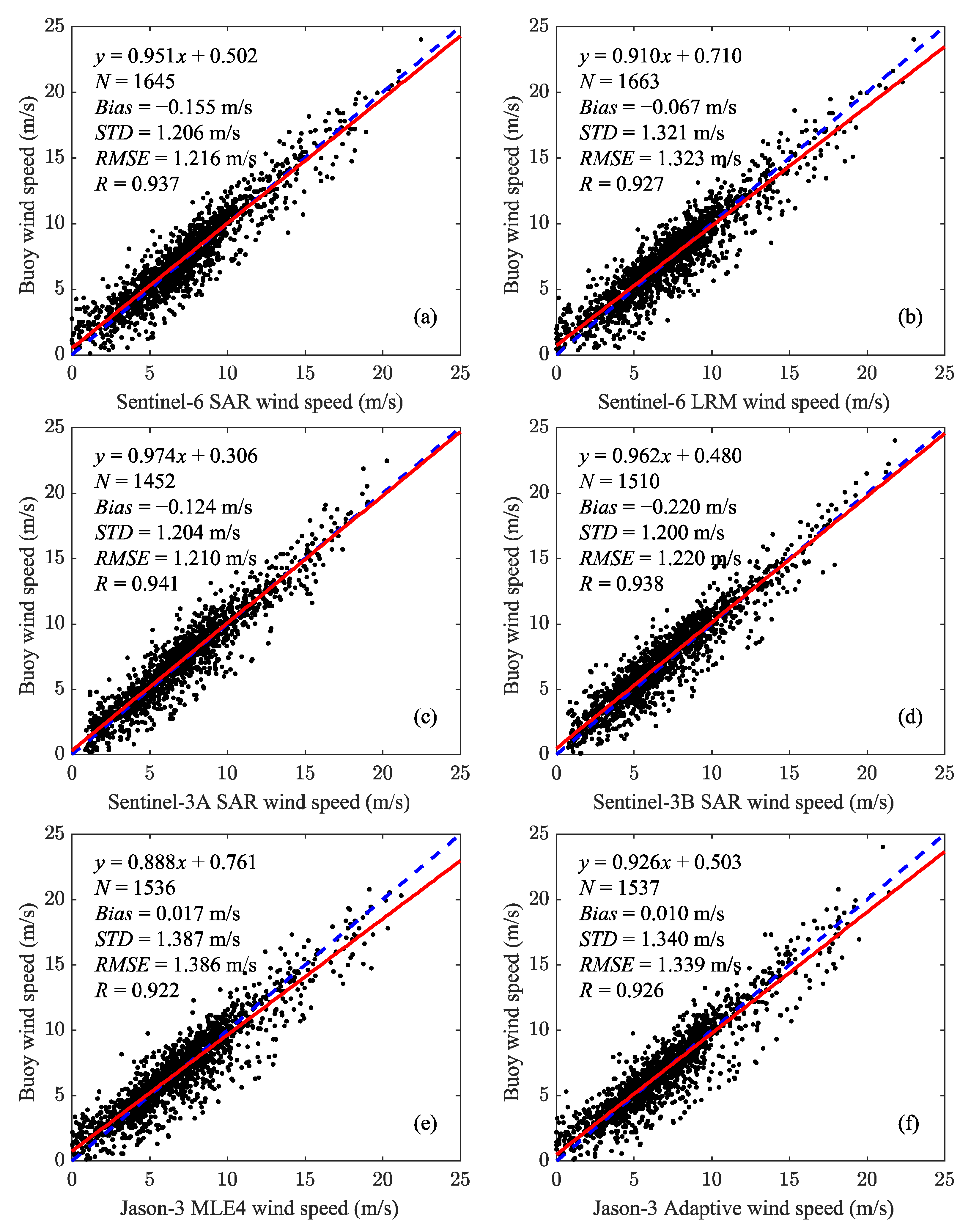
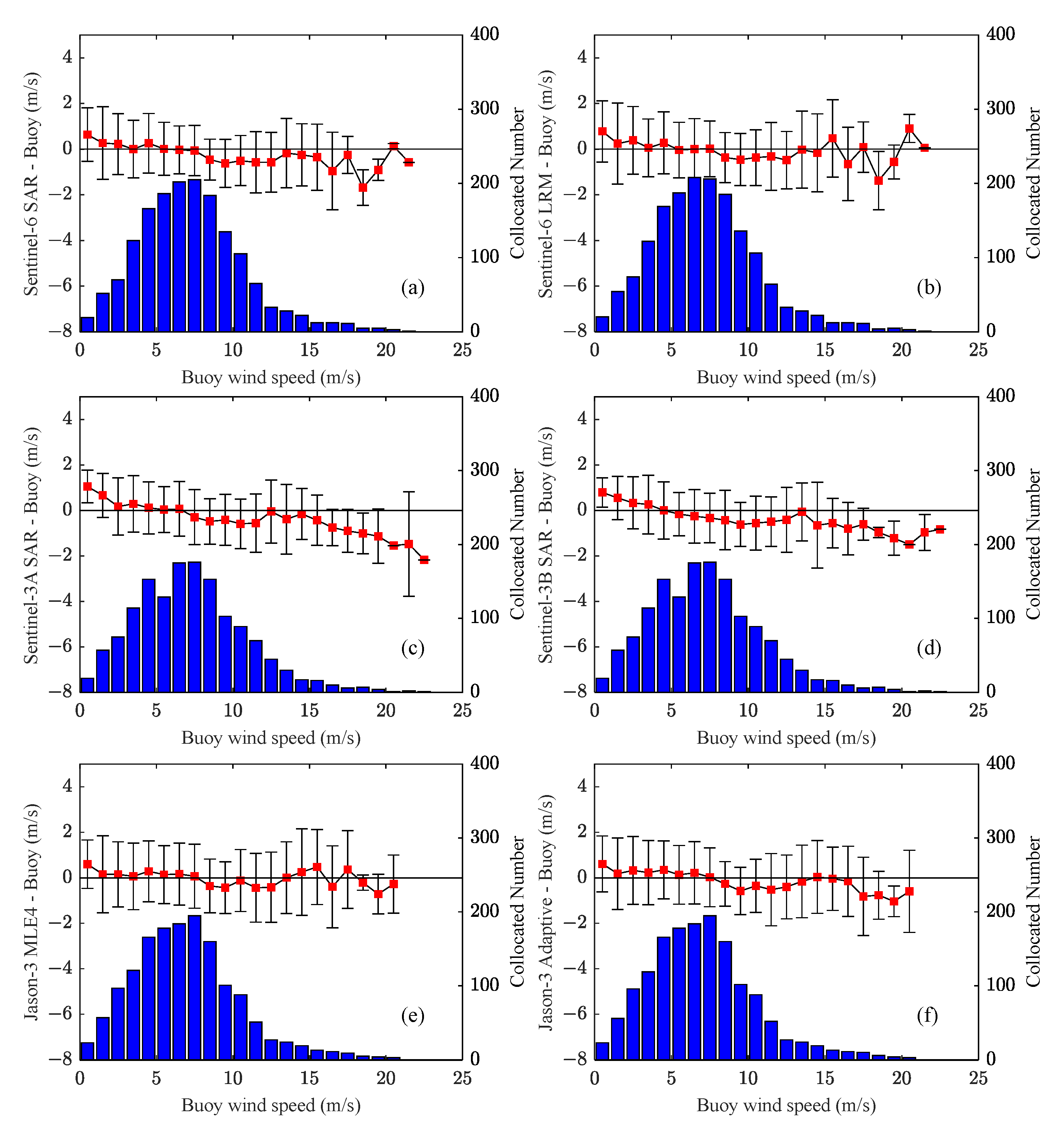
3.2.2. Comparison against NDBC Data

Figure 9 shows the scatterplots of Sentinel-6, Sentinel-3A/B and Jason-3 SWH measurements against the NDBC buoys. The red solid lines show the linear regressions obtained from the measurements. The valid number of the collocations is 1631 for the Sentinel-6 SARM, 1652 for Sentinel-6 LRM, 1523 for Sentinel-3A SARM and 1587 for Sentinel-3B SARM, 1617 for Jason-3 MLE4 re-tracking and 1620 for Jason-3 adaptive re-tracking. Sentinel-6 SARM SWH measurements have an RMSE of 0.361 m with a positive bias of 0.254 m, which is higher than Sentinel-6 LRM (RMSE: 0.225 m, bias: 0.004 m). The results for Sentinel-3A SARM measurements (RMSE: 0.284 m, bias: 0.093 m) are close to those for the Sentinel-3B SARM measurements (RMSE: 0.271 m, bias: 0.104 m). Jason-3 adaptive re-tracking measurements have the lowest RMSE (0.192 m) among the six data sets and almost no bias. The RMSE (0.241 m) of the Jason-3 MLE4 re-tracking measurements is close to the that of Sentinel-6 LRM measurements. The biases and STDs for the SARM measurements are higher than those for the LRM measurements on the whole.

To examine the dependency of the bias (altimeter minus buoy) between altimeter and buoy measurements, the number of collocations, bias and STDs are calculated within each 1 m buoy SWH bin from 0 to 10 m and presented in Figure 10. The histogram shows the number of collocations, the dotted line represents the trend of the bias and the error bar indicates the STD in each bin. Sentinel-6 SARM has positive biases at all SWH ranges. When SWH is below 4.5 m, the biases and STDs of Sentinel-6 SARM SWH increase with the increase in SWH. The SWH biases for Sentinel-6 LRM are close to 0 when SWH is below 4.5 m. Jason-3 MLE4 and Jason-3 adaptive re-tracking SWH measurements have similar results as Sentinel-6 LRM. Sentinel-3A and Sentinel-3B SWH measurements have higher biases than Sentinel-6 LRM but lower biases than Sentinel-6 SARM. When SWH is above 4.5 m, both Sentinel-6 SARM and Sentinel-6 LRM have relatively large biases.

Figure 11 shows the scatterplots of Sentinel-6, Sentinel-3A/B and Jason-3 wind speed measurements against the collocated NDBC buoys. There are 1645, 1663, 1452, 1510, 1536 and 1537 collocations for Sentinel-6 SARM, Sentinel-6 LRM, Sentinel-3A SARM, Sentinel-3B SARM, Jason-3 MLE4 re-tracking and Jason-3 adaptive re-tracking, respectively. The bias, STD, RMSE and R for the Sentinel-6 SARM measurements are -0.155 m/s, 1.206 m/s, 1.216 m/s and 0.937, respectively. The results for Sentinel-3A SARM (bias: −0.124 m/s, STD: 1.204 m/s, RMSE: 1.210 m/s) and Sentinel-3B SARM (bias: -0.220 m/s, STD: 1.200 m/s, RMSE: 1.220 m/s) are close to Sentinel-6 SARM. The bias, STD and RMSE of the Sentinel-6 LRM measurements are -0.067 m/s, 1.321 m/s and 1.323 m/s, respectively. Jason-3 MLE4 re-tracking measurements have a slightly higher RMSE (1.386 m/s) than Jason-3 adaptive re-tracking (1.339 m/s) but their biases are very close to each other. The biases and STDs for the SARM measurements are lower than those for the LRM measurements on the whole. Results in Yang et al. [40] also show that Sentinel-3A/3B (1.23 m/s) SARM wind speed measurements have lower RMSEs than Jason-3 (1.43 m/s) when compared against NDBC buoy measurements.

The differences in wind speed between of the altimeters and the buoys were analyzed as a function of wind speed, and the biases and STDs of the wind speed differences are illustrated with intervals of 1 m/s in Figure 12. The STDs for the SARM measurements are slightly lower than those for the LRM measurements. When wind speed is above 7.5 m/s, Sentinel-6 SARM and Sentinel-3A/B SARM have negative biases. The biases for Sentinel-6 LRM, Jason-3 MLE4 re-tracking and Jason-3 adaptive re-tracking are close to zero.

3.2.3. Comparison against Other Satellites

As shown in Figure 1, the spatial coverage of the NDBC buoys is poor and irregular, especially for the open ocean areas. Therefore, cross-comparison with other altimeters over the global ocean is necessary. In this study, we conducted a crossover comparison between Sentinel-6 and Sentinel-3A/B and Jason-3. To derive the collocated data, we computed the crossovers and then selected the crossovers, the time differences of which are no more than 0.5 h.

Figure 13 and Figure 14 show the SWH comparisons of Sentinel-6 against three other altimetry missions. Figure 13 presents the results for Sentinel-6 SARM measurements while Figure 14 presents Sentinel-6 LRM measurements. The agreement between Sentinel-6, Sentienl-3 and Jason-3 SWH measurements is very good and the correlation coefficients are all higher than 0.99. After 25 April 2022, there is no crossover whose time difference between Sentinel-6 and Jason-3 is less than 0.5 h because Jason-3 has changed to the interleaved position on the reference orbit. We can see that the Sentinel-6 LRM SWH data are more consistent with other missions than the Sentinel-6 SARM data. When compared to the Sentinel-6 SARM data, the RMSE is 0.315 m for Sentinel-3A SARM, 0.309 m for Sentinel-3B SARM, 0.489 m for Jason-3 MLE4 re-tracking and 0.524 m for Jason-3 adaptive re-tracking. As for the Sentinel-6 LRM data, the RMSE is reduced to 0.215 m for Sentinel-3A SARM, 0.224 m for Sentinel-3B SARM, 0.135 m for Jason-3 MLE4 re-tracking and 0.122 m for Jason-3 adaptive re-tracking.

Figure 15 and Figure 16 show wind speed comparisons of Sentinel-6 against three other altimetry missions. Figure 15 and Figure 16 are for Sentinel-6 SARM and LRM, respectively. When compared to the Sentinel-6 SARM, Jason-3 adaptive re-tracking (0.381 m/s) has the lowest RMSE while Jason-3 MLE4 re-tracking (0.811 m/s) has the largest RMSE among the four data sets. The biases and RMSEs for Sentinel-3A SARM (0.685 m/s) and Sentinel-3B SARM (0.647 m/s) are similar. As for the Sentinel-6 LRM, the RMSE is 0.839 m/s for Sentinel-3A SARM, 0.886 m/s for Sentinel-3B SARM, 0.423 m/s for Jason-3 MLE4 re-tracking and 0.682 m/s for Jason-3 adaptive re-tracking.

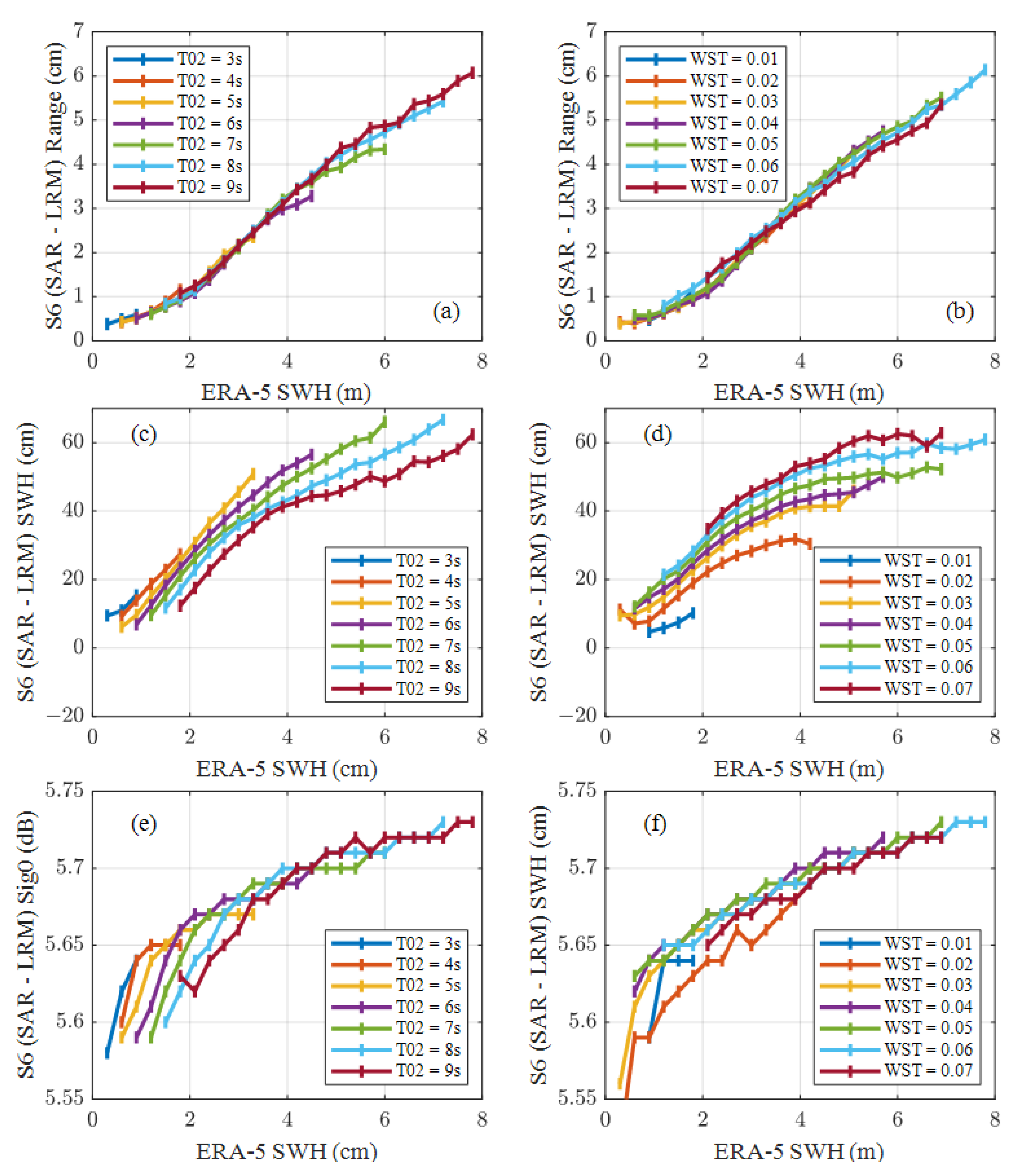
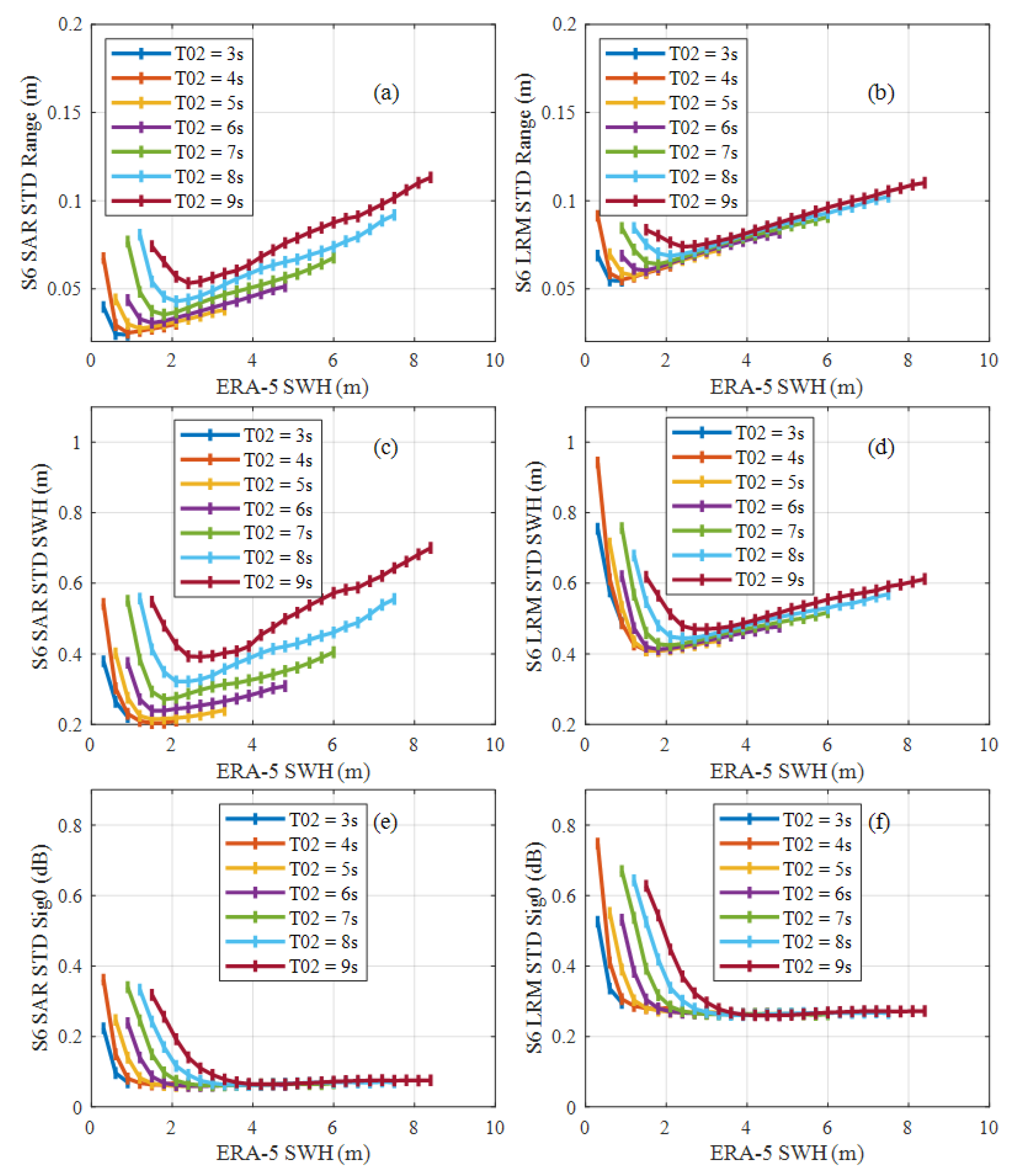
3.3. Impact of Ocean Waves on Parameter Retrievals from Sentinel-6 SARM Data

SARM has much higher along-track resolution (~300 m) than LRM. The ocean waves whose wavelength is a few hundred meters are not able to be fully measured in a ground strip. Therefore, the shape of the SARM waveforms may be distorted. This affects the final retrievals of parameters for the SAR altimeter. Moreau et al. [41] found that the long wavelength ocean wave can affect the SWH retrieval for the SAR altimeter through CryoSat-2 and simulation data analysis. In addition, the Doppler frequency of the radar signal can be affected by the ocean waves’ motion [42]. Egido et al. [43] analyzed the impact of the ocean waves’ motion on the SAR altimeters measurements using theoretical analysis and simulations. Surface motion increases the SWH bias. The noise in the range and SWH increases with the wavelength even if the surface is static. Amarouche et al. [44] analyzed the impact of waves’ motion on the SAR altimeters using Sentinel-3 real data analysis. Very good agreement has been found between the Sentinel-3 data analysis and theoretical analysis and simulations.

In this study, we aim to analyze the impact of ocean waves on range, SWH and sigma0 retrievals from Sentinel-6 SARM data. Several wave parameters (SWH, T02 and MWD) are derived from ERA5 re-analysis to assess the impact linked to time evolution of the short and long wavelengths but also to significant slope (correlated with vertical velocity).

The spectral moments are defined as [44,45]

$$m_x={\displaystyle \iint f^{x}S(f,\varphi )}dfd\varphi$$

(7)

where $S(f,\varphi )$ is the wave direction spectrum.

SWH is the mean of the highest third of wave heights and defined as

$$SWH=4\sqrt{m_0}$$

(8)

T02 is the mean time interval between zero up-crossings and defined as

$$T_{02}=2\pi \sqrt{\frac{m_0}{m_2}}$$

(9)

The spectral wave steepness (WST) is calculated using SWH and T02:

$$WST=\frac{2\pi SWH}{g{T}_{02}{}^2}$$

(10)

Figure 17 shows the Sentinel-6 range, SWH and sigma0 differences between the SARM and LRM estimations. The range difference increases with the increase in SWH but variations with T02 and WST are not clearly visible. The SWH difference increases with the increase in SWH and variations with T02 and WST are clearly visible. For a given SWH, the SWH differences with T02 and WST may vary by as much as 5–20 cm. When SWH is less than 3 m, the sigma0 difference increases with SWH and variations with T02 and WST are clearly visible. Above 3 m of SWH, the sigma0 difference increases with the increase in SWH but variations with T02 and WST are not obvious. As shown in Amarouche et al. [44], effects of vertical velocity are dominant at high wave steepness values or low wave period values while effects of long wavelengths are dominant at low wave steepness values and high wave period values. For a given SWH value, when the wave period increases, the wavelength also increases, then the SWH bias decreases. On the other hand, when the wave steepness increases, the vertical velocity increases, which leads to the increase in the horizontal Doppler shift, then the SWH bias increases.

Figure 18 and Figure 19 show the STDs of 20 Hz range, SWH and sigma0 measurements derived from Sentinel-6 SARM and LRM data. For small SWH values (<3 m), the STDs of the 20 Hz range, SWH and sigma0 measurements derived from SARM and LRM depend on SWH, T02 and WST. Large variations with respect to T02 and WST are observed. Above 3 m of SWH, the STDs of the 20 Hz range and SWH measurements derived from SARM depend on SWH, T02 and WST and variations with T02 and WST are clearly visible. For the LRM data, variations of the STDs of the range and SWH measurements with T02 and WST are not clearly visible. The STDs of the 20 Hz sigma0 measurements have nearly no variations with SWH and T02 for both SARM and LRM data. For a given SWH value, when the wave period increases, the wavelength and swell effects also increase, then the range noise and SWH variability increase. On the other hand, when the wave steepness increases, the vertical velocity increases and swell effects decrease, then the range noise and SWH variability decrease.

Figure 20 shows the STDs of the 20 Hz range, SWH and sigma0 measurements for different relative azimuth directions and T02 values. The relative azimuth direction is computed by subtracting the satellite flight direction from the ERA5 mean wave direction [46]. A second-order harmonic fit ($\mathrm{a}0+\mathrm{a}1\cos \left(\mathrm{z}\right)+\mathrm{a}2\cos \left(2\mathrm{z}\right)$) is conducted and presented in the figure. Besides SWH and T02, the STDs of the 20 Hz SARM range and SWH measurements also depend on the relative azimuth direction. The STDs of the 20 Hz SARM range and SWH measurements are higher when the wave propagation direction is parallel to the satellite flight direction than those when the two directions are perpendicular. The reason for this phenomenon is that the footprint of SARM is asymmetric. The 20 Hz STDs of Sentinel-6 LRM range and SWH are less sensitive to the relative azimuth direction because the footprint of LRM is circularly symmetric. Unlike range and SWH, variations of the STDs of the 20 Hz SARM and LRM sigma0 measurements with the relative azimuth direction are not clearly visible. Similar results can be found in Xu et al. [46], which analyzes the influence of the anisotropic effects of the ocean wave surface on SAR altimetry backscatter coefficient measurements.

4. Discussion

Poseidon-4 onboard S6-MF is the first SAR altimeter that uses an interleaved mode. In this study, we assessed the Sentinel-6 SARM and LRM products for the SSH, SWH and wind speed measurements.

We first assessed the SSH measurements using range noise, SLA PSD and crossover analysis. The 20 Hz range noise at 2 m SWH is 3.07 cm for Sentinel-6 SARM data and 6.40 cm for Sentinel-6 LRM data. A value of 0.70 cm is obtained for the Sentinel-6 SARM 1 Hz range noise, which is better than the value for Sentinel-3A/B SARM (1.08 cm), Jason-3 MLE4 re-tracking (1.59 cm) and Jason-3 adaptive re-tracking (1.46 cm) at 2 m SWH. The SLA PSD analysis shows that the Sentinel-6 SARM data have lower range noise than the other three missions. Crossover analysis results also show that the Sentinel-6 SARM data have good performance. The STD of the Sentinel-6 SARM SSH differences at crossovers over the ocean is 3.76 cm, which is slightly lower than those for Sentinel-3A SARM (4.00 cm) and Sentinel-3B SARM (3.96 cm). The STD of the SSH crossover difference for Sentinel-6 LRM (4.27 cm) is very close to the value for Jason-3 MLE4 re-tracking (4.29 cm) and Jason-3 adaptive re-tracking (4.27 cm).

We then assessed the SWH and wind speed measurements in terms of noise, comparison against NDBC buoy data and other altimetry missions. The SWH noise for Sentinel-6 SARM data is better than the value for Sentinel-3A SARM and Sentinel-3B SARM but higher than Jason-3 adaptive re-tracking data. When compared to the NBDC SWH measurements, the Sentinel-6 SARM has an RMSE of 0.361 m with a positive bias of 0.254 m. The RMSE for Sentinel-6 SARM data is higher than Sentinel-3A SARM (RMSE: 0.284 m, bias: 0.093 m) and Sentine-3B SARM (RMSE: 0.271 m, bias: 0.104 m) data due to its higher bias. The Sentinel-6 LRM data have an RMSE of 0.225 m with a bias of 0.004 m, which is close to the Jason-3 MLE4 re-tracking (RMSE: 0.241 m, bias: 0.026 m) and higher than the Jason-3 adaptive re-tracking (RMSE: 0.192 m, bias: 0.006 m) data. The sigma0 noise for the Sentinel-6 SARM data is the lowest among the six data sets. When compared to the NBDC wind speed measurements, the Sentinel-6 SARM has an RMSE of 1.216 m/s with a negative bias of 0.155 m/s, which is close to the value for Sentinel-3A SARM data (RMSE: 1.210 m/s, bias: −0.124 m/s) and Sentinel-3B SARM (RMSE: 1.220 m/s, bias: −0.220 m/s), Sentinel-6 LRM (RMSE: 1.323 m/s, bias: -0.067 m/s), Jason-3 MLE4 re-tracking (RMSE: 1.386 m/s, bias: 0.017 m/s) and Jason-3 adaptive re-tracking (RMSE: 1.339 m/s, bias: 0.010 m/s) data. Comparison against other missions indicates that the SWH and wind speed measurements derived from the Sentinel-6 SARM and LRM data have good consistency with those derived from other altimetry missions.

We also analyzed the impacts of ocean waves on range, SWH and sigma0 retrievals from Sentinel-6 SARM data. SWH and sigma0 differences between the SARM and LRM data both highly depend on SWH, T02 and WST while the range difference is highly dependent on SWH but not highly dependent on T02 and WST. The 20 Hz SARM range and SWH STDs are highly dependent on SWH, T02 and WST. Furthermore, the 20 Hz SARM range and SWH also depend on the relative azimuth direction (higher range and SWH STDs are observed when the wave propagation direction is parallel to the satellite flight direction).

5. Conclusions

The S6-MF satellite was launched on 21st November 2020. Poseidon-4 onboard S6-MF is the first SAR altimeter that uses an interleaved mode. The interleaved mode performs a near continuous transmission of Ku-band pulses, that allows SAR and pulse limited data to be gathered simultaneously. In this study, we assessed the Sentinel-6 SARM and LRM products for the SSH, SWH and wind speed measurements. Results show the good performance of the Sentinel-6 SSH measurements. The Sentinel-6 SARM data have a lower 20 Hz range noise level than Sentinel-3A/B SARM, Sentinel-6 LRM and Jason-3 data. The STD of the SSH differences at crossovers for Sentinel-6 SARM is lower than the value for Sentinel-3A/B SARM, Sentinel-6 LRM and Jason-3. Comparison against NDBC SWH measurements shows that the Sentinel-6 SARM has a higher RMSE with respect to Sentinel-3A/B SARM, Sentinel-6 LRM and Jason-3. Comparison against NDBC wind speed measurements shows that the RMSE for Sentinel-6 SARM is close to Sentinel-3A/B SARM and lower than Sentinel-6 LRM and Jason-3. However, the range, SWH and sigma0 retrievals from Sentinel-6 SARM data are sensitive to SWH, T02, WST and relative azimuth direction. The Sentinel-6 SARM data’s sensitivity to long wavelength and vertical velocity should be paid attention to in the future.

References

1. Legeais, J.; Ablain, M.; Zawadzki, L.; Zuo, H.; Johannessen, J.A.; Scharffenberg, M.G.; Fenoglio-Marc, L.; Fernandes, M.J.; Andersen, O.B.; Rudenko, S.; et al. An improved and homogeneous altimeter sea level record from the ESA Climate Change Initiative. Earth Syst. Sci. Data 2018, 10, 281–301. [Google Scholar] [CrossRef] [Green Version]
2. Karimi, A.A.; Ghobadi-Far, K.; Passaro, M. Barystatic and steric sea level variations in the Baltic Sea and implications of water exchange with the North Sea in the satellite era. Front. Mar. Sci. 2022, 9, 963564. [Google Scholar] [CrossRef]
3. Li, Z.; Guo, J.; Ji, B.; Wan, X.; Zhang, S. A Review of Marine Gravity Field Recovery from Satellite Altimetry. Remote Sens. 2022, 14, 4790. [Google Scholar] [CrossRef]
4. Wang, Z.; Chao, N.; Chao, D. Using satellite altimetry leveling to assess the marine geoid. Geod. Geodyn. 2020, 11, 106–111. [Google Scholar] [CrossRef]
5. Fan, D.; Li, S.; Li, X.; Yang, J.; Wan, X. Seafloor Topography Estimation from Gravity Anomaly and Vertical Gravity Gradient Using Nonlinear Iterative Least Square Method. Remote Sens. 2021, 13, 64. [Google Scholar] [CrossRef]
6. Lyard, F.H.; Allain, D.J.; Cancet, M.; Carrère, L.; Picot, N. FES2014 global ocean tide atlas: Design and performance. Ocean Sci. 2021, 17, 615–649. [Google Scholar] [CrossRef]
7. Quartly, G.D. Removal of Covariant Errors from Altimetric Wave Height Data. Remote Sens. 2019, 11, 2319. [Google Scholar] [CrossRef] [Green Version]
8. Yu, F.; Qi, J.; Jia, Y.; Chen, G. Evaluation of HY-2 Series Satellites Mapping Capability on Mesoscale Eddies. Remote Sens. 2022, 14, 4262. [Google Scholar] [CrossRef]
9. Jiang, L.; Schneider, R.; Andersen, O.; Bauer-Gottwein, P. CryoSat-2 Altimetry Applications over Rivers and Lakes. Water 2017, 9, 211. [Google Scholar] [CrossRef]
10. Jiang, L.; Nielsen, K.; Dinardo, S.; Andersen, O.B.; Bauer-Gottwein, P. Evaluation of Sentinel-3 SRAL SAR altimetry over Chinese rivers. Remote Sens. Environ. 2020, 237, 111546. [Google Scholar] [CrossRef]
11. Jiang, L.; Nielsen, K.; Andersen, O.B.; Bauer-Gottwein, P. Monitoring recent lake level variations on the Tibetan Plateau using CryoSat-2 SARIn mode data. J. Hydrol. 2017, 544, 109–124. [Google Scholar] [CrossRef] [Green Version]
12. Laxon, S.W.; Giles, K.A.; Ridout, A.L.; Wingham, D.J.; Willatt, R.; Cullen, R.; Kwok, R.; Schweiger, A.; Zhang, J.; Haas, C.; et al. CryoSat-2 estimates of Arctic sea ice thickness and volume. Geophys. Res. Lett. 2013, 40, 732–737. [Google Scholar] [CrossRef] [Green Version]
13. Lawrence, I.R.; Armitage, T.W.K.; Tsamados, M.C.; Stroeve, J.C.; Dinardo, S.; Ridout, A.L.; Muir, A.; Tilling, R.L.; Shepherd, A. Extending the Arctic sea ice freeboard and sea level record with the Sentinel-3 radar altimeters. Adv. Space Res. 2021, 68, 711–723. [Google Scholar] [CrossRef]
14. Kwok, R.; Cunningham, G.F. Variability of Arctic sea ice thickness and volume from CryoSat-2. Philos. Trans. A Math Phys. Eng. Sci. 2015, 373, 20140157. [Google Scholar] [CrossRef]
15. Shepherd, A.; Ivins, E.R.; Geruo, A.; Barletta, V.R.; Bentley, M.J.; Bettadpur, S.; Briggs, K.H.; Bromwich, D.H.; Forsberg, R.; Galin, N.; et al. A Reconciled Estimate of Ice-Sheet Mass Balance. Science 2012, 338, 1183–1189. [Google Scholar] [CrossRef] [Green Version]
16. Shepherd, A.; Gilbert, L.; Muir, A.S.; Konrad, H.; McMillan, M.; Slater, T.; Briggs, K.H.; Sundal, A.V.; Hogg, A.E.; Engdahl, M.E. Trends in Antarctic Ice Sheet Elevation and Mass. Geophys. Res. Lett. 2019, 46, 8174–8183. [Google Scholar] [CrossRef] [Green Version]
17. Su, X.; Shum, C.K.; Guo, J.; Duan, J.; Howat, I.; Yi, Y. High resolution Greenland ice sheet inter-annual mass variations combining GRACE gravimetry and Envisat altimetry. Earth Planet. Sc. Lett. 2015, 422, 11–17. [Google Scholar] [CrossRef]
18. Raney, R.K. The Delay/Doppler Radar Altimeter. IEEE T. Geosci. Remote 1998, 5, 1578–1588. [Google Scholar] [CrossRef]
19. Peng, F.; Deng, X. Validation of Sentinel-3A SAR mode sea level anomalies around the Australian coastal region. Remote Sens. Environ. 2020, 237, 111548. [Google Scholar] [CrossRef]
20. Boy, F.; Desjonqueres, J.; Picot, N.; Moreau, T.; Raynal, M. CryoSat-2 SAR-Mode Over Oceans: Processing Methods, Global Assessment, and Benefits. Ieee T. Geosci. Remote. 2017, 55, 148–158. [Google Scholar] [CrossRef]
21. Raynal, M.; Labroue, S.; Moreau, T.; Boy, F.; Picot, N. From conventional to Delay Doppler altimetry: A demonstration of continuity and improvements with the Cryosat-2 mission. Adv. Space Res. 2018, 62, 1564–1575. [Google Scholar] [CrossRef]
22. Laforge, A.; Fleury, S.; Dinardo, S.; Garnier, F.; Remy, F.; Benveniste, J.; Bouffard, J.; Verley, J. Toward improved sea ice freeboard observation with SAR altimetry using the physical retracker SAMOSA+. Adv. Space Res. 2021, 68, 732–745. [Google Scholar] [CrossRef]
23. McMillan, M.; Muir, A.; Shepherd, A.; Escolà, R.; Roca, M.; Aublanc, J.; Thibaut, P.; Restano, M.; Ambrozio, A.; Benveniste, J. Sentinel-3 Delay-Doppler altimetry over Antarctica. Cryosphere 2019, 13, 709–722. [Google Scholar] [CrossRef] [Green Version]
24. Abileah, R.; Vignudelli, S. Precise inland surface altimetry (PISA) with nadir specular echoes from Sentinel-3: Algorithm and performance assessment. Remote Sens. Environ. 2021, 264, 112580. [Google Scholar] [CrossRef]
25. Wingham, D.J.; Francis, C.R.; Baker, S.; Bouzinac, C.; Brockley, D.; Cullen, R.; de Chateau-Thierry, P.; Laxon, S.W.; Mallow, U.; Mavrocordatos, C.; et al. CryoSat: A mission to determine the fluctuations in Earth’s land and marine ice fields. Adv. Space Res. 2006, 37, 841–871. [Google Scholar] [CrossRef]
26. Donlon, C.; Berruti, B.; Buongiorno, A.; Ferreira, M.H.; Féménias, P.; Frerick, J.; Goryl, P.; Klein, U.; Laur, H.; Mavrocordatos, C.; et al. The Global Monitoring for Environment and Security (GMES) Sentinel-3 mission. Remote Sens. Environ. 2012, 120, 37–57. [Google Scholar] [CrossRef]
27. Donlon, C.J.; Cullen, R.; Giulicchi, L.; Vuilleumier, P.; Francis, C.R.; Kuschnerus, M.; Simpson, W.; Bouridah, A.; Caleno, M.; Bertoni, R.; et al. The Copernicus Sentinel-6 mission: Enhanced continuity of satellite sea level measurements from space. Remote Sens. Environ. 2021, 258, 112395. [Google Scholar] [CrossRef]
28. Yang, J.; Zhang, J. Validation of Sentinel-3A/3B Satellite Altimetry Wave Heights with Buoy and Jason-3 Data. Sensors 2019, 19, 2914. [Google Scholar] [CrossRef] [Green Version]
29. Li, X.; Xu, Y.; Liu, B.; Lin, W.; He, Y.; Liu, J. Validation and Calibration of Nadir SWH Products From CFOSAT and HY-2B With Satellites and In Situ Observations. J. Geophys. Res. Ocean. 2021, 126, e2020JC016689. [Google Scholar] [CrossRef]
30. Durden, S.; Vesecky, J. A physical radar cross-section model for a wind-driven sea with swell. Ieee J. Ocean. Eng. 1985, 10, 445–451. [Google Scholar] [CrossRef]
31. Hersbach, H.; Bell, B.; Berrisford, P.; Hirahara, S.; Horányi, A.; Muñoz Sabater, J.; Nicolas, J.; Peubey, C.; Radu, R.; Schepers, D.; et al. The ERA5 global reanalysis. Q. J. Roy. Meteor. Soc. 2020, 146, 1999–2049. [Google Scholar] [CrossRef]
32. Bignalet-Cazalet, F.; Picot, N.; Desai, S.; Scharroo, R.; Egido, A. Jason-3 Products Handbook. Available online: https://www.aviso.altimetry.fr/fileadmin/documents/data/tools/hdbk_j3.pdf (accessed on 29 November 2022).
33. Calafat, F.M.; Cipollini, P.; Bouffard, J.; Snaith, H.; Féménias, P. Evaluation of new CryoSat-2 products over the ocean. Remote Sens. Environ. 2017, 191, 131–144. [Google Scholar] [CrossRef]
34. Jiang, M.; Xu, K.; Liu, Y. Calibration and Validation of Reprocessed HY-2A Altimeter Wave Height Measurements Using Data from Buoys, Jason-2, Cryosat-2, and SARAL/AltiKa. J. Atmos. Ocean. Tech. 2018, 35, 1331–1352. [Google Scholar] [CrossRef]
35. Bronner, E.; Picot, N.; Carrère, L.; Desai, S.; Desjonquères, J.; Tran, N. Jason-1 Products Handbook. Available online: https://www.aviso.altimetry.fr/fileadmin/documents/data/tools/hdbk_j1_gdr.pdf (accessed on 29 November 2022).
36. Jia, Y.; Yang, J.; Lin, M.; Zhang, Y.; Ma, C.; Fan, C. Global Assessments of the HY-2B Measurements and Cross-Calibrations with Jason-3. Remote Sens. 2020, 12, 2470. [Google Scholar] [CrossRef]
37. Dibarboure, G.; Boy, F.; Desjonqueres, J.D.; Labroue, S.; Lasne, Y.; Picot, N.; Poisson, J.C.; Thibaut, P. Investigating Short-Wavelength Correlated Errors on Low-Resolution Mode Altimetry. J. Atmos. Ocean. Tech. 2014, 31, 1337–1362. [Google Scholar] [CrossRef] [Green Version]
38. Ablain, M.; Philipps, S.; Picot, N.; Bronner, E. Jason-2 Global Statistical Assessment and Cross-Calibration with Jason-1. Mar. Geod. 2010, 33, 162–185. [Google Scholar] [CrossRef]
39. Zanifé, O.Z.; Vincent, P.; Amarouche, L.; Dumont, J.P.; Thibaut, P.; Labroue, S. Comparison of the Ku-Band Range Noise Level and the Relative Sea-State Bias of the Jason-1, TOPEX, and Poseidon-1 Radar Altimeters. Mar. Geod. 2003, 26, 201–238. [Google Scholar] [CrossRef]
40. Yang, J.; Zhang, J.; Jia, Y.; Fan, C.; Cui, W. Validation of Sentinel-3A/3B and Jason-3 Altimeter Wind Speeds and Significant Wave Heights Using Buoy and ASCAT Data. Remote Sens. 2020, 12, 2079. [Google Scholar] [CrossRef]
41. Moreau, T.; Tran, N.; Aublanc, J.; Tison, C.; Le Gac, S.; Boy, F. Impact of long ocean waves on wave height retrieval from SAR altimetry data. Adv. Space Res. 2018, 62, 1434–1444. [Google Scholar] [CrossRef]
42. Boisot, O.; Amarouche, L.; Lalaurie, J.; Guérin, C. Dynamical Properties of Sea Surface Microwave Backscatter at Low-Incidence: Correlation Time and Doppler Shift. Ieee T. Geosci. Remote. 2016, 54, 7385–7395. [Google Scholar] [CrossRef]
43. Egido, A.; Ray, C. Impact of the Ocean Waves Motion on the Delay-Doppler Altimeters Measurements. Available online: https://ostst.aviso.altimetry.fr/fileadmin/user_upload/2019/IPM_03_Egido20191022_-_OSTST_-_AEE.pdf (accessed on 29 November 2022).
44. Amarouche, L.; Tran, N.; Boy, F. Impact of the Ocean Waves on the Delay/Doppler Altimeters: Analysis Using Real Sentinel-3 Data. Available online: https://ostst.aviso.altimetry.fr/fileadmin/user_upload/tx_ausyclsseminar/files/TranetAl_DopplerWaves_DataAnalysis_OSTST_2020.pdf (accessed on 29 November 2022).
45. Buchhaupt, C.; Fenoglio, L.; Becker, M.; Kusche, J.R. Impact of vertical water particle motions on focused SAR altimetry. Adv. Space Res. 2021, 68, 853–874. [Google Scholar] [CrossRef]
46. Xu, X.; Xu, K.; Jiang, M.; Geng, B.; Shi, L. Investigation of the Anisotropic Patterns in the Altimeter Backscatter Measurements Over Ocean Wave Surfaces. Front. Earth Sci. 2021, 9, 1–14. [Google Scholar] [CrossRef]
Figure 1. Locations of the NDBC buoys used in this study.
Remotesensing 15 00012 g001
Figure 2. Sentinel-6 (a) 20 Hz and (b) 1 Hz range noises and their comparisons with Sentinel-3A/B and Jason-3 missions.
Remotesensing 15 00012 g002
Figure 3. Sea level anomaly spectra of Sentinel-6 (a) 20-Hz SLA and (b) 1 Hz SLA and their comparisons with Jason-3 and Sentinel-3A/B missions.
Remotesensing 15 00012 g003
Figure 4. Maps of Sentinel-6 SSH crossover differences for (a) SARM and (b) LRM from November 2021 to October 2022 (Cycle 37 to Cycle 71).
Remotesensing 15 00012 g004
Figure 5. Month per month monitoring of (a) mean and (b) STD of SSH crossover differences for Sentinel-6, Sentinel-3A/B and Jason-3.
Remotesensing 15 00012 g005
Figure 6. Month per month monitoring of the (a) mean and (b) STD of the SSH differences computed at Sentinel-6 (SARM) and Sentinel-3A/B and Jason-3 crossovers.
Remotesensing 15 00012 g006
Figure 7. Month per month monitoring of the (a) mean and (b) STD of the SSH differences computed at Sentinel-6 (LRM) and Sentinel-3A/B and Jason-3 crossovers.
Remotesensing 15 00012 g007
Figure 8. Sentinel-6 20 Hz (a) SWH noise and (b) sigma0 noise and their comparisons with Sentinel-3A/B and Jason-3 missions.
Remotesensing 15 00012 g008
Figure 9. Scatterplots of (a) Sentinel-6 SARM, (b) Sentinel-6 LRM, (c) Sentinel-3A SARM, (d) Sentinel-3B SARM, (e) Jason-3 MLE4 and (f) Jason-3 adaptive SWH measurements against the collocated NDBC buoys.
Remotesensing 15 00012 g009
Figure 10. Bias dependency of altimeters and buoy SWH measurements for (a) Sentinel-6 SARM, (b) Sentinel-6 LRM, (c) Sentinel-3A SARM, (d) Sentinel-3B SARM, (e) Jason-3 MLE4 and (f) Jason-3 adaptive SWH measurements.
Remotesensing 15 00012 g010
Figure 11. Scatterplots of (a) Sentinel-6 SARM, (b) Sentinel-6 LRM, (c) Sentinel-3A SARM, (d) Sentinel-3B SARM, (e) Jason-3 MLE4 and (f) Jason-3 adaptive wind speed measurements against the collocated NDBC buoys.
Remotesensing 15 00012 g011
Figure 12. Bias dependency of altimeters and buoy wind speed measurements for (a) Sentinel-6 SARM, (b) Sentinel-6 LRM, (c) Sentinel-3A SARM, (d) Sentinel-3B SARM, (e) Jason-3 MLE4 and (f) Jason-3 adaptive wind speed measurements.
Remotesensing 15 00012 g012
Figure 13. Scatterplots of Sentinel-6 SWH measurements in SARM against (a) Sentinel-3A SARM, (b) Sentinel-3B SARM, (c) Jason-3 MLE-4 and (d) Jason-3 adaptive re-tracking measurements.
Remotesensing 15 00012 g013
Figure 14. Scatterplots of Sentinel-6 SWH measurements in LRM against (a) Sentinel-3A SARM, (b) Sentinel-3B SARM, (c) Jason-3 MLE-4 and (d) Jason-3 adaptive re-tracking measurements.
Remotesensing 15 00012 g014
Figure 15. Scatterplots of Sentinel-6 wind speed measurements in SARM against (a) Sentinel-3A SARM, (b) Sentinel-3B SARM, (c) Jason-3 MLE-4 and (d) Jason-3 adaptive re-tracking measurements.
Remotesensing 15 00012 g015
Figure 16. Scatterplots of Sentinel-6 wind speed measurements in LRM against (a) Sentinel-3A SARM, (b) Sentinel-3B SARM, (c) Jason-3 MLE-4 and (d) Jason-3 adaptive re-tracking measurements.
Remotesensing 15 00012 g016
Figure 17. Bin-averaged values of Sentinel-6 (SARM minus LRM) (a,b) range, (c,d) SWH and (e,f) sigma0 against ERA5 SWH estimates for different T02 (left) and WST (right) values.
Remotesensing 15 00012 g017
Figure 18. STDs of 20 Hz Sentinel-6 SARM (left) and LRM (right) range, SWH and sigma0 against ERA5 SWH estimates for seven different T02 values.
Remotesensing 15 00012 g018
Figure 19. STDs of 20 Hz Sentinel-6 SARM (left) and LRM (right) range, SWH and sigma0 against ERA5 SWH estimates for seven different WST values.
Remotesensing 15 00012 g019
Figure 20. STDs of 20 Hz Sentinel-6 SARM (left) and LRM (right) range, SWH and sigma0 against ERA5 SWH estimates for different relative azimuth direction and T02 values.
Remotesensing 15 00012 g020