Deep Unfolded Gridless DOA Estimation Networks Based on Atomic Norm Minimization

Abstract

Deep unfolded networks have recently been regarded as an essential way to direction of arrival (DOA) estimation due to the fast convergence speed and high interpretability. However, few consider gridless DOA estimation. This paper proposes two deep unfolded gridless DOA estimation networks to resolve the above problem. We first consider the atomic norm-based 1D and decoupled atomic norm-based 2D gridless DOA models solved by the alternating iterative minimization of variables, respectively. Then, the corresponding deep networks are trained offline after constructing the corresponding complete training datasets. At last, the trained networks are applied to realize the 1D DOA and 2D estimation, respectively. Simulation results reveal that the proposed networks can secure higher 1D and 2D DOA estimation performances while maintaining a lower computational expenditure than typical methods.

1. Introduction

The Direction of Arrival (DOA) estimation technique is widely used in radar, sonar, and other fields, and is an important research direction in array signal processing [1,2]. Typical DOA estimation methods include MUSIC (Multiple Signal Classification) [3] and ESPRIT (Estimation of Signal Parameters via Rotational Invariance Technique) [4]. Thanks to the successful application of 1D DOA estimation problems, the subspace super-resolution algorithms are successfully extended to 2D DOA estimation problems, such as 2D unitary estimation of signal parameters via rotational invariance techniques (U-ESPRIT) [5] and the 2D multiple signal classification (2D MUSIC) algorithm [6]. These algorithms can obtain high angular resolution under the requirement of multiple snapshot reception data and known coherent signal sources, but any of the conditions not satisfied will cause its estimation performance to degrade or even fail.

In recent years, effective alternative algorithms based on compressive sensing techniques have been introduced into the field of DOA estimation, and fruitful research results have been achieved. The traditional compressed sensing algorithms, for example, orthogonal matching pursuit (OMP) [7], sparse Bayesian learning (SBL) [8], and other algorithms, divide the possible space of the signal source into a finite number of grid points by dimension. It shows excellent estimation performance when the target angle falls exactly on the established grid, which can be applied to complex scenarios such as single snapshot, signal coherence, and missing data. On the contrary, if the real signal source does not fall on the established grid, it will cause a grid mismatch problem, and the estimation performance will be degraded or even fail. In addition, traditional compressed sensing algorithms must satisfy the pairwise isometry property (PIP) [9] and high-density gridding.

A gridless continuous compressive sensing technique based on the atomic norm theory and the Vandermonde decomposition theorem is proposed to overcome these problems, called atomic norm minimization (ANM) [10,11,12,13,14]. ANM projects the Vandermonde structure of the steering matrix from the observed data to the corresponding semi-definite programming (SDP) model using the Toeplitz matrix and obtains the recovered signal by solving the SDP optimization model to achieve super-resolution. Compared with the conventional compressed sensing algorithm, it does not need to mesh the space domain, and effectively avoids the grid mismatch problem and the PIP limitation. By solving the SDP optimization model using the SDPT3-based CVX/alternating direction method of multipliers (ADMM), the ANM-based method can obtain the recovered signal to achieve super-resolution 1D DOA estimation. However, computational budgets of the CVX solver SDPT3-based method increase with the scale of the problem. The performance of the model-driven ADMM method also depends on the selected regularization parameters, and improper initial values of the parameters affect its convergence speed and accuracy.

According to Caratheodory’s theory, the Vandermonde decomposition of the Toeplitz matrix does not hold in higher dimensional spaces, so the 1D ANM cannot be directly extended to the 2D DOA estimation problem. Fortunately, Chi et al. successfully apply vectorized ANM (VANM) to 2D DOA estimation with a dual Toeplitz matrix with a 2-dimensional Vandermonde structure [15]. However, the vectorization operations increase computational complexity. They cannot be applied to real-world scenarios. The dual 2D ANM starts from the dual problem of the VANM, but does not reduce the high computational costs of the VANM [16]. Luckily, Tian et al. proposed a new decoupled atomic norm minimization algorithm (DANM) [17,18,19] to reduce the heavy computational burden. DANM first replaces the vector atomic set in VANM with the matrix atomic set and then derives the corresponding SDP model, which naturally decouples the dual Toeplitz matrix in VANM into two Toeplitz matrices containing one-dimensional Vandermonde structures. Thereby, the 2D DOA estimation problem is converted to two 1D DOA estimation problems. This algorithm significantly reduces the computational complexity and is several orders of magnitude lower than VANM, which can also be solved by SDPT3-based CVX and ADMM algorithms [20,21]. However, ADMM algorithms are suffering from difficulties of parameter setting in practical applications. Meanwhile, inappropriate parameter settings will decrease the convergence speed and accuracy of the ADMM algorithm, thus adding to the computing complexity and degrading the DOA estimation performance. Even if the proper parameters can be chosen by theoretical analysis and cross-validation method, the fixed parameter settings fail to guarantee optimal convergence.

Recently, the Deep Unfolding/Unrolling (DU) method has been proposed as a solution to the above problems of model-driven SR algorithms inspired by deep learning techniques. With the DU method, a specific SR algorithm is unrolled into a deep neural network by taking the number of iterations of the algorithm as the number of layers and the algorithm’s parameters as the network’s learning parameters. SR-Net is trained on the training data set to determine the optimal parameters, thus improving the convergence speed and accuracy of the SR algorithm [22,23,24,25,26,27,28,29,30,31]. Some deep unfolding networks have successfully solved different DOA estimation problems. For example, The paper implemented fast DOA estimation under array deficiencies using the learned ISTA (LISTA) algorithm based on the iterative soft thresholding algorithm (ISTA) [32]; The paper proposed (position-enabled complex Toeplitz learned iterative shrinkage thresholding algorithm) PACT-LISTA algorithm, which integrates the intrinsic Toeplitz structure of the signal into LISTA, ignores the amplitude and phase information of the signal to be recovered and solves the mutual coupling problem between the antenna array elements using data [33]; In the paper [34], the iterative fixed-point continuation (FPC) algorithm was expanded into a deep neural network DeepFPC, to achieve single-bit DOA estimation. The paper in [35] modeled the 2D-DOA estimation problem for unmanned vehicles as a block sparse recovery problem and then used sparse bayesian learning network (SBLNet) to learn nonlinear features from data received by a large-scale (Multi-Input Multi-Output) MIMO multiple-input system or (Reconfigurable Intelligent Surface) RIS to achieve 2D-DOA and polarization parameter estimation at lower computational complexity. Our group extended the smoothed (SL0) algorithm into SL0-Net to achieve super-resolution DOA estimation [36]. By combining model-driven and data-driven approaches effectively, these DU methods reduce computational complexity dramatically and provide high DOA performance compared with corresponding SR algorithms.

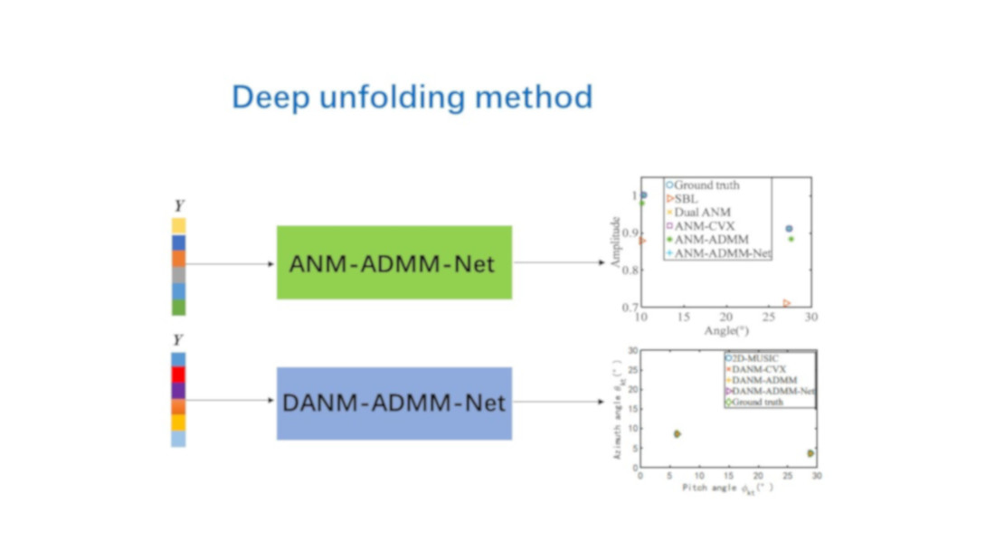
Based on the ideas above, this paper proposes the DU gridless DOA estimation method, and the main ideas and contributions are as follows:

➀

The ANM-ADMM and DANM-ADMM algorithms are implemented to solve the 1D ANM and 2D DANM gridless DOA model, respectively, based on sparse optimization theory to reduce the computational burden of the existing SDPT3-based CVX method to a certain extent.

➁

Aiming to reduce the high computational cost and tackle the problems of intractable parameter presettings of the algorithms, we unfold the algorithms to the multi-layer deep neural network named ANM-ADMM-Net and DANM-ADMM-Net, respectively, based on the DU method. They include several types of network layers and parameters. Depending on the ANM and DANM estimation models, the complete and reasonable dataset construction methods are proposed to train the network with suitable training methods to achieve fast and accurate 1D and 2D DOA estimation, respectively.

➂

Traditional DU methods, such as FISTA and LAMP, are challenging to solve the ANM and DANM models. The proposed ANM-ADMM-Net and DANM-ADMM-Net as the novel DU-DOA framework is the only DU method that can optimize the above models and secure better gridless 1D and 2D DOA estimation performances with lower operational complexity.

The rest of this paper is structured as follows: In Section 2, the array received signal model and gridless DOA model, including the ANM and DANM models, are established briefly. Section 3 introduces the 1D ANM-ADMM and 2D DANM-ADMM algorithms first, then, the network structure, datasets construction method, and training methods of ANM-ADMM-Net and DANM-ADMM-Net are provided in detail. Section 4 verifies the performance and advantages of DU-DOA through simulation experiments compared with the SDPT3-based CVX and ADMM methods. Conclusions are drawn in Section 5.

2. Signal Model and ANM-DOA Model

2.1. 1D Signal Model and Its ANM-DOA Model

Assume that $K_t$ far-field narrow-band signals incident into a uniform linear array (ULA) composed of $M$ array elements. Then, the array received signal can be characterized as

$$\begin{array}{cc}\mathit{Y}\hfill & =\mathit{X}+N\hfill \\ & ={\displaystyle {\sum }_{k_t=1}^{K_t}\mathit{a}\left(f_{k_t}\right){\mathit{s}}_{k_t}}+N\hfill \\ & ={\displaystyle {\sum }_{k_t=1}^{K_t}{c}_{k_t}\mathit{a}\left(f_{k_t}\right){\mathit{b}}_{k_t}}+N\hfill \end{array}$$

(1)

where $\mathit{a}(f_{k_t})={[1,\exp (\mathrm{j}2\pi f_{k_t}),\cdots ,\exp (\mathrm{j}2\pi (M-1)f_{k_t})]}^{\mathrm{T}}$ is the steering vector, $f_{k_t}=d\sin {\theta }_{k_t}/\lambda$$=\sin {\theta }_{k_t}/2$, $\lambda$ is the signal wavelength, $d=\lambda /2$ is the array spacing, ${\theta }_{k_t}$ is the angle between the $k_t$-th signal source and the array, and ${[\cdot ]}^{\mathrm{T}}$ represents the transposition; ${\mathit{s}}_{k_t}=[s_{k_{t}1},s_{k_{t}2},\cdots ,s_{k_{t}L}]\in {ℂ}^{1\times L}$ is the complex amplitude matrix; $c_{k_t}=||{\mathit{s}}_{k_t}|{|}_2>0$ and ${\mathit{b}}_{k_t}=c_{k_t}^{-1}{\mathit{s}}_{k_t}$ with $||{\mathit{b}}_{k_t}|{|}_2=1$; $N$ is the zero-mean Gaussian matrix white noise.

According to ANM theory [10], the received signal $\mathit{X}$ can be seen as a linear combination of some $K_t$ atoms in the set ${\mathit{A}}_M$. The set ${\mathit{A}}_M$ of atoms can be defined as

$${\mathit{A}}_M\triangleq \left\{\mathit{A}\right(f_{k_t},{\mathit{b}}_{k_t})=\mathit{a}\left(f_{k_t}\right){\mathit{b}}_{k_t},f_{k_t}\in [0,0.5]\}$$

(2)

Then, the atomic norm ${\mathit{l}}_0$ of $\mathit{X}$ is defined as

$$||\mathit{X}|{|}_{{\mathit{A}}_M,0}=\underset{K_t}{\inf }\left\{K_t|\mathit{X}={\displaystyle \sum _{k_t=1}^{K_t}{c}_{k_t}\mathit{A}(f_{k_t},{\mathit{b}}_{k_t})},f_{k_t}\in {\mathit{A}}_M,c_{k_t}\ge 0\right\}$$

(3)

So, the frequency can be recovered by dealing with the following optimization problem

$$\underset{\mathit{X}}{\mathrm{argmin}}||\mathit{X}|{|}_{{\mathit{A}}_M,0}s.t.||\mathit{Y}-\mathit{X}|{|}_2^2\le \epsilon$$

(4)

Usually, the solution of (4) can be obtained by its dual problem [34,37]. By exploiting the semi-positive, Toeplitz, and low-rank properties of the array covariance matrix $\mathit{R}=\mathrm{E}\{\mathit{Y}{\mathit{Y}}^{\mathrm{H}}\}=T\left(\mathit{u}\right)$ [10], also (4) can be formulated into the following SDP problem.

$$\underset{\mathit{W},\mathit{u},\mathit{X}}{\min }\frac{1}{2}[\mathrm{Tr}(\mathit{W})+\mathrm{Tr}(T(\mathit{u}))]s.t.\left[\begin{array}{cc}T(\mathit{u})& \mathit{X}\\ {\mathit{X}}^{\mathrm{H}}& \mathit{W}\end{array}\right]\ge 0,||\mathit{Y}-\mathit{X}|{|}_{\mathrm{F}}^2\le \epsilon$$

(5)

where $\mathrm{E}\{\cdot \}$ and $\mathrm{Tr}(\cdot )$ denote the expectation operator and the trace operation, and $T(\cdot )$ denotes a mapping operation from a vector $\mathit{u}\in {ℂ}^{M\times 1}$ to a Hermitian Toeplitz matrix $T(\mathit{u})\in {ℂ}^{M\times M}$, and $\mathit{W}\in {ℂ}^{L\times L}$ denotes an auxiliary variable matrix.

For problem (5), CVX solver SDPT3 can be utilized to secure optimal $T(\mathit{u})$ efficiently [38]. Then, the results of DOA are estimated by Vandermonde composition of $T(\mathit{u})$ [34,37]. Although completely avoiding gridding, the dual ANM and ANM-CVX methods have extensive computational complexity, failing to meet real-time requirements.

2.2. 2D Signal Model and Its DANM-DOA Model

Consider $K_t$ spatial far-field narrowband signals acting on a $N\times M$ uniform rectangular array (URA) with array element spacing of half wavelength, as shown in Figure 1. The pitch angle ${\varphi }_{k_t}$ and azimuth angle ${\theta }_{k_t}$ of the $k_t$-th incident signals are related to the angles ${\alpha }_{k_t}$ and ${\beta }_{k_t}$ between the $x$ and $y$ axes as follows:

$${\varphi }_{k_t}=\arcsin (\sqrt{\sin {}_2({\alpha }_{k_t})+\sin {}_2({\beta }_{k_t})})$$

(6)

$${\theta }_{k_t}=\arctan (\frac{\sin ({\beta }_{k_t})}{\sin ({\alpha }_{k_t})}$$

(7)

By finding the angles ${\alpha }_{k_t}$ and ${\beta }_{k_t}$, we can obtain ${\theta }_{k_t}$ and ${\varphi }_{k_t}$ according to Equations (6) and (7). Therefore, this paper uses ${\alpha }_{k_t}$ and ${\beta }_{k_t}$ for signal modeling analysis. Then, the array guiding vector, the guiding matrix of dimensions $x$ and $y$ are

$$\{\begin{array}{l}{\mathit{a}}_x(w_{x,k_t})={[1,{\mathrm{e}}^{-\mathrm{j}{w}_{x,k_t}},\cdots ,{\mathrm{e}}^{-\mathrm{j}(N-1)w_{x,k_t}}]}^{\mathrm{T}}\\ {\mathit{a}}_y(w_{y,k_t})={[1,{\mathrm{e}}^{-\mathrm{j}{w}_{y,k_t}},\cdots ,{\mathrm{e}}^{-\mathrm{j}(M-1)w_{y,k_t}}]}^{\mathrm{T}}\end{array}$$

(8)

$$\{\begin{array}{l}{\mathit{A}}_x=[{\mathit{a}}_x(w_{x,1}),{\mathit{a}}_x(w_{x,2}),\cdots ,{\mathit{a}}_x(w_{x,K_t})]\\ {\mathit{A}}_y=[{\mathit{a}}_y(w_{y,1}),{\mathit{a}}_y(w_{y,2}),\cdots ,{\mathit{a}}_y(w_{y,K_t})]\end{array}$$

(9)

The single snapshot data can be expressed as:

$$\mathit{X}={\displaystyle \sum _{k_t=1}^{K_t}{\mathit{s}}_{k_t}{\mathit{a}}_x(w_{x,k_t}){\mathit{a}}_y^{\mathrm{T}}(w_{y,k_t})}={\mathit{A}}_x\mathit{S}{\mathit{A}}_y^{\mathrm{T}}$$

(10)

where $\mathit{S}=\mathrm{diag}(s_1,s_2,\cdots ,s_{K_t})$ is a diagonal amplitude matrix, and $s_{k_t}$ is the amplitude of the $k_t$-th target signal corresponding to the true frequencies of interest $w_{x,k_t}=\pi \sin {\varphi }_{k_t}\cos {\theta }_{k_t}=\pi \sin {\alpha }_{k_t}$ and $w_{y,k_t}=\pi \sin {\varphi }_{k_t}\sin {\theta }_{k_t}=\pi \sin {\beta }_{k_t}$. Two dimensional frequencies sets are ${\mathit{w}}_x=(w_{x,1},w_{x,2},\cdots ,w_{x,K_t})$, ${\mathit{w}}_y=(w_{y,1},w_{y,2},\cdots ,w_{y,K_t})$, and the corresponding angles are $\widehat{\mathit{\alpha }}=({\alpha }_1,{\alpha }_2,\cdots ,{\alpha }_{K_t})$, $\widehat{\mathit{\beta }}=({\beta }_1,{\beta }_2,\cdots ,{\beta }_{K_t})$.

2D DOA estimation means that $w_{x,k_t}$ and $w_{y,k_t}$ are first recovered from the observations data $\mathit{X}$, then arriving at the angles ${\alpha }_{k_t}$ and ${\beta }_{k_t}$ for acquiring pitch angle ${\varphi }_{k_t}$ and azimuth angle ${\theta }_{k_t}$.

According to [17], the set of atoms ${\mathit{A}}_V$ in a matrix form of the received signal data $\mathit{X}$ can be expressed as

$$\begin{array}{cc}\hfill {\mathit{A}}_M& =\{{\mathit{a}}_x(w_{x,k_t}){\mathit{a}}_y^{\mathrm{T}}(w_{y,k_t}),w_{x,k_t},w_{y,k_t}\in [-\pi ,\pi ]\}\hfill \\ & =\{{\mathit{A}}_{\gamma },\gamma \in [-\pi ,\pi ]\times [-\pi ,\pi ]\}\hfill \end{array}$$

(11)

where each atom is a rank l matrix. The atomic norm ${\mathit{l}}_1$ of $\mathit{X}$ is defined as

$$||\mathit{X}|{|}_{{\mathit{A}}_M}=\inf \left\{{\displaystyle \sum _{k_t}^{K_t}|{\mathit{s}}_{k_t,p}|}|\mathit{X}={\displaystyle \sum _{k_t}^{K_t}\mathit{A}(\gamma ){\mathit{s}}_{k_t}},\mathit{A}(\gamma )\in {\mathit{A}}_M\right\}$$

(12)

Define the one-level Toeplitz matrices $T({\mathit{u}}_x)$ and $T({\mathit{u}}_y)$ constructed by their first rows ${\mathit{u}}_x\in {ℂ}^{M\times 1}$, and ${\mathit{u}}_y\in {ℂ}^{N\times 1}$, respectively. The problem of minimizing Equation (12) can be transformed into addressing the following semidefinite programming (SDP) problem [19]

$$\begin{array}{l}\underset{{\mathit{u}}_x,{\mathit{u}}_y,\mathit{X}}{\arg \min }\frac{\lambda }{2\sqrt{NM}}\mathrm{Tr}(T({\mathit{u}}_x))+\mathrm{Tr}(T({\mathit{u}}_y))\\ s.t.\mathit{\Theta }=\left[\begin{array}{cc}T({\mathit{u}}_x)& {\mathit{X}}_{}^{\mathrm{H}}\\ {\mathit{X}}_{}& T({\mathit{u}}_y)\end{array}\right]\ge 0,||\mathit{Y}-\mathit{X}|{|}_{\mathrm{F}}^2\le \epsilon \end{array}$$

(13)

where $\mathit{Y}$ denotes the received data with noise.

After obtaining $T({\mathit{u}}_x)$ and $T({\mathit{u}}_y)$, the $x$ and $y$-dimensional DOA can be obtained by the following decomposition

$$T({\mathit{u}}_x)={\mathit{A}}_x{\mathit{D}}_x{\mathit{A}}_x^{\mathrm{H}},T({\mathit{u}}_y)={\mathit{A}}_y{\mathit{D}}_y{\mathit{A}}_y^{\mathrm{H}}$$

(14)

where ${\mathit{D}}_x$ and ${\mathit{D}}_y$ are diagonal matrices. The final 2D DOA is obtained by the pairing procedure after obtaining the DOA in each dimension [39].

For the DANM optimization model (13), an off-the-shelf CVX solver SDPT3 can be utilized to secure $T({\mathit{u}}_x)$ and $T({\mathit{u}}_y)$, where the dimensionality of the semi-definite constraint matrix is $(N+M)\times (N+M)$ [21]. The above directly leads to high computational costs when the dimensions $N$ and $M$ are unacceptably large. Although the ADMM algorithm in [20,40] is an alternative to solving (13), computational load still needs reconsidered.

3. DU-DOA Estimation

In order to lighten the computational load and enhance the estimation performance efficiently, this paper intends to the DU-DOA method to solve (5) for 1D DOA and (13) for the 2D DOA estimations in this section. According to [22], the DU approach can be seen as an iterative step based on the SR algorithm for designing the structure and parameters of the deep neural network. DU methods such as LISTA, LAMP, and LePOM [22,23,24] can all theoretically achieve the 2D DOA estimation. However, these methods are unsuitable for solving the AMM-DOA and DAMM-DOA models, i.e., (5) and (13). This paper analyzes the ANM-ADMM and the DANM-ADMM algorithms to address the above problem in Section 3.1 and Section 3.3, respectively. The algorithms are expanded into the deep neural network ANM-ADMM-Net and DANM-ADMM-Net to achieve fast and accurate 1D and 2D DOA estimation in Section 3.2 and Section 3.4, respectively.

3.1. 1D ANM-ADMM DOA

To facilitate the solution, (5) is rewritten as (15).

$$\begin{array}{l}[\mathit{X},\mathit{u}]=\underset{\mathit{X},\mathit{W},\mathit{u},\mathit{\Theta }}{\arg \min }\frac{\tau }{2}[\mathrm{Tr}(\mathit{W})+\mathrm{Tr}(T(\mathit{u}))]+\frac{1}{2}||\mathit{Y}-\mathit{X}|{|}_{\mathrm{F}}^2\\ s.t.\mathit{\Theta }=\left[\begin{array}{cc}T(\mathit{u})& \mathit{X}\\ {\mathit{X}}^{\mathrm{H}}& \mathit{W}\end{array}\right]\ge 0\end{array}$$

(15)

where $\tau \in ℝ$ is the regularization factor.

The augmented Lagrangian function of the problem (15) can be defined via [41].

$$\begin{array}{l}\underset{\mathit{X},\mathit{W},\mathit{u},\mathit{\Theta }\ge 0,\mathbf{\Lambda }}{\arg \min }\frac{\tau }{2}[\mathrm{Tr}(\mathit{W})+\mathrm{Tr}(T(\mathit{u}))]+\frac{1}{2}||\mathit{Y}-\mathit{X}|{|}_{\mathrm{F}}^2\\ +\langle \mathbf{\Lambda },\mathit{\Theta }-\left[\begin{array}{cc}T(\mathit{u})& \mathit{X}\\ {\mathit{X}}^{\mathrm{H}}& \mathit{W}\end{array}\right]\rangle +\frac{\rho }{2}{\Vert \mathit{\Theta }-\left[\begin{array}{cc}T(\mathit{u})& \mathit{X}\\ {\mathit{X}}^{\mathrm{H}}& \mathit{W}\end{array}\right]\Vert }_{\mathrm{F}}^2\\ =\underset{\mathit{X},\mathit{W},\mathit{u},\mathit{\Theta }\ge 0,\mathbf{\Lambda }}{\arg \min }\frac{\tau }{2}[\mathrm{Tr}(\mathit{W})+\mathrm{Tr}(T(\mathit{u}))]+\frac{1}{2}||\mathit{Y}-\mathit{X}|{|}_2^2+\Delta \end{array}$$

(16)

where $\mathbf{\Lambda }\in {ℂ}^{(M+L)\times (M+L)}$ is the Lagrangian multiplier, and $\rho >0$ is the penalty factor.

Note (16) is an unconstrained optimization problem, so that given the received signal $\mathit{Y}$, unknown signal components $\mathit{X}$, and vector $\mathit{u}$ can be estimated by alternatively minimizing the cost function of $\mathit{X}$, $\mathit{W}$, $\mathit{u}$, $\mathit{\Theta }$ and $\mathbf{\Lambda }$ [14]. The specific iterative process can be found in Appendix A.

In conclusion, the ADMM algorithm for solving (5) is provided in Algorithm 1.

Algorithm 1: ANM-ADMM-DOA algorithm.

Input:$\mathit{Y}$, iterations $K$, penalty factor $\rho$, regularization factor $\tau$. Initialization:${\mathit{\Theta }}^{(0)}={\mathbf{0}}_{M+L}$ and ${\mathbf{\Lambda }}^{(0)}={\mathbf{0}}_{M+L}$. For $k=0:K-1$ do  (1) ${\mathit{X}}^{(k+1)}=1/(1+2\rho )(\mathit{Y}+2{\mathbf{\Lambda }}_{\mathit{X}}^{(k)}+2\rho {\mathit{\Theta }}_{\mathit{X}}^{(k)})$;  (2) ${\mathit{W}}^{(k+1)}={\rho }^{-1}{\mathbf{\Lambda }}_{\mathit{W}}^{(k)}+{\mathit{\Theta }}_{\mathit{W}}^{(k)}-\tau /(2\rho ){\mathbf{I}}_L$;  (3) ${\mathit{u}}^{(k+1)}=\mathbf{\Gamma }(T^{\ast }({\rho }^{-1}{\mathbf{\Lambda }}_{T(\mathit{u})}^{(k)}+{\mathit{\Theta }}_{T(\mathit{u})}^{(k)})-\tau /(2\rho )M{\mathit{e}}_1)$;  (4) $\{\begin{array}{l}{\widehat{\mathit{\Theta }}}^{(k+1)}=\left[\begin{array}{cc}T({\mathit{u}}^{(k+1)})& {\mathit{X}}^{(k+1)}\\ {({\mathit{X}}^{(k+1)})}^{\mathrm{H}}& {\mathit{W}}^{(k+1)}\end{array}\right]-{\rho }^{-1}{\mathbf{\Lambda }}^{(k)}\\ {\widehat{\mathit{\Theta }}}^{(k+1)}=\mathit{G}\mathrm{diag}(\{{\delta }_g\}){\mathit{G}}^{-1},{\mathit{\Theta }}^{(k+1)}=\mathit{G}\mathrm{diag}({\{{\delta }_g\}}_{+}){\mathit{G}}^{-1}\end{array}$;  (5) ${\mathbf{\Lambda }}^{(k+1)}={\mathbf{\Lambda }}^{(k)}+\rho \left({\mathit{\Theta }}^{(k+1)}-\left[\begin{array}{cc}T({\mathit{u}}^{(k+1)})& {\mathit{X}}^{(k+1)}\\ {({\mathit{X}}^{(k+1)})}^{\mathrm{H}}& {\mathit{W}}^{(k+1)}\end{array}\right]\right)$; End Output: Recovered signal of interest ${\mathit{X}}^{(K)}$, the optimal estimate ${\mathit{u}}^{(K)}$. Then: Estimate $f_{k_t}$ and ${\mathit{s}}_{k_t}$ by Vandermonde decomposition of $T({\mathit{u}}^{(K)}\sqrt{M}/2)$ and compute DOA by ${\theta }_{k_t}=\mathrm{asind}(2f_{k_t})$.

According to the above derivation, the parameters of the model-driven ADMM algorithm, including the penalty factor $\rho$ and the regularization factor $\tau$, need to be set in advance, which is a challenge for practical applications. Meanwhile, inappropriate parameter settings will decrease the convergence speed and accuracy of the ADMM algorithm, thus adding to the computing complexity of (5) and degrading the DOA estimation performance. Even if the proper parameters can be chosen by theoretical analysis and cross-validation method [41], the fixed parameter settings fail to guarantee the optimal convergence of the ANM-ADMM algorithm. Based on the idea of the DU method, this paper expands the algorithm into a deep neural network ANM-ADMM-Net and learns its optimal parameters from the constructed data obeying a particular distribution, thus solving the above problems.

It is necessary to note that the optimal estimates $T({\mathit{u}}^{(K)})$ of the algorithm are the critical points of the following estimation. Therefore, we can consider the output as a label and construct a proper loss function in the next subsection.

3.2. 1D ANM-ADMM-Net DOA

For the optimization problem shown in (5), when the system parameters are given and the complex amplitude and noise all obey a particular distribution, the received data $\mathit{Y}$ will also have a particular distribution. At this point, assume that an optimal set of parameter sequences exists so that (5) can be solved quickly and accurately by the ADMM algorithm for all received signals, with the DOA obeying a specific distribution. Therefore, this subsection constructs the network ANM-ADMM-Net to tackle the problems of the ADMM algorithm based on its iterative steps. This network couples the interpretability of the model-driven algorithm and the nonlinear fitting capability of the data-driven deep learning method. Training networks based on a sufficient and complete training data set can obtain optimal iterative parameters, thereby reducing the number of iterations and further enabling higher speed and ameliorated performance of DOA estimation. In the following, the four parts of ANM-ADMM-Net: network structures, dataset construction, network initialization, and training are described thoroughly.

3.2.1. Network Structure

According to the steps in Algorithm 1, the ANM-ADMM algorithm can be mapped to a $K$ layer network ANM-ADMM-Net shown in Figure 2, whose inputs are $\mathit{Y}$, ${\mathit{\Theta }}^{(\mathbf{0})}={\mathbf{0}}_{M+L}$, and ${\mathbf{\Lambda }}^{(0)}=0_{M+L}$, and the learnable parameters are $\mathbf{\Omega }={\left\{{\mathbf{\Omega }}^{(k+1)}\right\}}_{k=0}^{K-1}={\{{\rho }_{k+1},{\tau }_{k+1},{\eta }_{k+1}\}}_{k=0}^{K-1}$, to arrive at the signal components ${\mathit{X}}^{(K)}$ and the Toeplitz matrix $T({\mathit{u}}^{(K)})$. The $(k+1)$-th layer operation of ANM-ADMM-Net can be expressed as

$$[{\mathit{X}}^{(k+1)},{\mathit{u}}^{(k+1)}]=F_{k+1}\{\mathit{Y},{\mathit{X}}^{(k)},{\mathit{W}}^{(k)},{\mathit{u}}^{(k)},{\theta }^{(k)},{\mathbf{\Lambda }}^{(k)},{\mathbf{\Omega }}^{(k+1)}\}$$

(17)

where $F_{k+1}\{\cdot \}$ contains five main structural sub-layers, including reconstruction sub-layer ${\mathbf{A}}^{(k+1)}$, the auxiliary variable update sub-layer ${\mathbf{B}}^{(k+1)}$, the Toeplitz transform sub-layer ${\mathbf{C}}^{(k+1)}$, the nonlinear sub-layer ${\mathbf{D}}^{(k+1)}$, and the multiplier update sub-layer ${\mathbf{E}}^{(k+1)}$ corresponding to (17). The specific description is as follows.

(1)

Reconstruction sub-layer ${\mathbf{A}}^{(k+1)}$: Taking the output ${\mathbf{\Lambda }}_x^{(k)}$ of the sub-layer ${\mathbf{E}}^{(k)}$ and ${\mathit{\Theta }}_x^{(k)}$ of the sub-layer ${\mathbf{D}}^{(k)}$ of $k$-th layer and received signal $\mathit{Y}$ as the input, the output ${\mathit{X}}^{(k+1)}$ is updated as

$${\mathit{X}}^{(k+1)}=1/(1+2{\rho }_{k+1})(\mathit{Y}+2{\mathbf{\Lambda }}_{\mathit{X}}^{(k)}+2{\rho }_{k+1}{\mathit{\Theta }}_x^{(k)})$$

(18)

where ${\rho }_{k+1}$ is the learnable parameter. The output ${\mathit{X}}^{(k+1)}$ of ${\mathbf{A}}^{(k+1)}$ can be used as the input of the sub-layer ${\mathbf{D}}^{(k+1)}$ and ${\mathbf{E}}^{(k+1)}$ in the $(k+1)$-th layer.

(2)

Auxiliary variable update sub-layer ${\mathbf{B}}^{(k+1)}$: Taking the output ${\mathit{\Theta }}_{\mathit{W}}^{(k)}$ of the sub-layer ${\mathbf{D}}^{(k+1)}$ and ${\mathbf{\Lambda }}_{\mathit{W}}^{(k)}$ of the sub-layer ${\mathbf{E}}^{(k)}$ in the $k$-th layer are used as inputs, the output of ${\mathbf{B}}^{(k+1)}$ is given by

$${\mathit{W}}^{(k+1)}={\rho }_{k+1}^{-1}{\mathbf{\Lambda }}_{\mathit{W}}^{(k)}+{\mathit{\Theta }}_{\mathit{W}}^{(k)}-{\tau }_{k+1}/(2{\rho }_{k+1}){\mathbf{I}}_L$$

(19)

where ${\tau }_{k+1}$ is the learnable parameter. The output ${\mathit{W}}^{(k+1)}$ is the input of the sub-layer ${\mathbf{D}}^{(k+1)}$ and ${\mathbf{E}}^{(k+1)}$ in the $(k+1)$-th layer.

(3)

Toeplitz transform sub-layer ${\mathbf{C}}^{(k+1)}$: The output ${\mathit{\Theta }}_{T(\mathit{u})}^{(k)}$ of the sub-layer ${\mathbf{D}}^{(k+1)}$ and ${\mathbf{\Lambda }}_{T(\mathit{u})}^{(k)}$ of the sub-layer ${\mathbf{E}}^{(k)}$ in the $k$-th layer are used as inputs, and the output is represented by

$${\mathit{u}}^{(k+1)}=\mathbf{\Gamma }(T^{\ast }({\rho }_{k+1}^{-1}{\mathbf{\Lambda }}_{T(\mathit{u})}^{(k)}+{\mathit{\Theta }}_{T(\mathit{u})}^{(k)})-{\tau }_{k+1}/(2{\rho }_{k+1})M{\mathit{e}}_1)$$

(20)

where ${\mathit{u}}^{(k+1)}$ can be the input of the sub-layer ${\mathbf{D}}^{(k+1)}$ and ${\mathbf{E}}^{(k+1)}$ in the $(k+1)$-th layer.

(4)

Nonlinear sub-layer ${\mathbf{D}}^{(k+1)}$: Taking the output ${\mathbf{\Lambda }}_{T(\mathit{u})}^{(k)}$ of the sub-layer ${\mathbf{E}}^{(k)}$ of the $k$-th layer, the output ${\mathit{X}}^{(k+1)}$ of the sub-layer ${\mathbf{A}}^{(k)}$, and the output ${\mathit{u}}^{(k+1)}$ of the sub-layer ${\mathbf{B}}^{(k+1)}$ as the input, the output of ${\mathbf{D}}^{(k+1)}$ can be given as

$$\{\begin{array}{l}{\widehat{\mathit{\Theta }}}^{(k+1)}=\left[\begin{array}{cc}T({\mathit{u}}^{(k+1)})& {\mathit{X}}^{(k+1)}\\ {({\mathit{X}}^{(k+1)})}^{\mathrm{H}}& {\mathit{W}}^{(k+1)}\end{array}\right]-{\rho }_{k+1}^{-1}{\mathbf{\Lambda }}^{(k)}\\ {\widehat{\mathit{\Theta }}}^{(k+1)}=\mathit{G}\mathrm{diag}(\{{\delta }_g\}){\mathit{G}}^{-1},{\mathit{\Theta }}^{(k+1)}=\mathit{G}\mathrm{diag}({\left\{{\delta }_g\right\}}_{+}){\mathit{G}}^{-1}\end{array}$$

(21)

where the output ${\mathit{\Theta }}^{(k+1)}$ of ${\mathbf{D}}^{(k+1)}$ can be used as the input of the sub-layer ${\mathbf{A}}^{(k+2)}$, ${\mathbf{B}}^{(k+2)}$, and ${\mathbf{C}}^{(k+2)}$ in the $(K+2)$-th layer.

(5)

Multiplier update sub-layer ${\mathbf{E}}^{(k+1)}$: Taking the output ${\mathbf{\Lambda }}^{(k)}$ of the sub-layer ${\mathbf{D}}^{(k)}$ of the $k$-th layer, the output ${\mathit{X}}^{(k+1)}$, ${\mathit{W}}^{(k+1)}$, ${\mathit{u}}^{(k+1)}$ and ${\mathit{\Theta }}^{(k+1)}$ of the sub-layer ${\mathbf{A}}^{(k+1)}$, ${\mathbf{B}}^{(k+1)}$, ${\mathbf{C}}^{(k+1)}$ and ${\mathbf{D}}^{(k+1)}$ respectively as input, the output of ${\mathbf{E}}^{(k+1)}$ can be updated by

$${\mathbf{\Lambda }}^{(k+1)}={\mathbf{\Lambda }}^{(k)}+{\eta }_{k+1}\left({\mathit{\Theta }}^{(k+1)}-\left[\begin{array}{cc}T({\mathit{u}}^{(k+1)})& {\mathit{X}}^{(k+1)}\\ {({\mathit{X}}^{(k+1)})}^{\mathrm{H}}& {\mathit{W}}^{(k+1)}\end{array}\right]\right)$$

(22)

where the multiplier update rate ${\eta }_{k+1}$ is the learnable parameter, and the output ${\mathbf{\Lambda }}^{(k+1)}$ of ${\mathbf{E}}^{(k+1)}$ can be used as the input in the $(k+2)$-th layer. It is essential to emphasize that the new parameters ${\eta }_{k+1}$ are added to enhance the learning capability further and the performance of ANM-ADMM-Net compared to updating multipliers by $\rho$ of ANM-ADMM (as shown in Algorithm 1).

Considering that each sub-layer’s parameters are learned and tuned, there will be $3K$ parameters for $K$ layer ANM-ADMM-Net generally, i.e., $\{{\rho }_1,\cdots ,{\rho }_k\}$, $\{{\tau }_1,\cdots ,{\tau }_k\}$, $\{{\eta }_1,\cdots ,{\eta }_k\}$. Compared with the ANM-ADMM algorithm, where the parameters ${\rho }_1=\cdots ={\rho }_k$ and ${\tau }_1=\cdots ={\tau }_k$ are fixed, this parameter learning strategy of ANM-ADMM-Net has the advantages of superior flexibility and brilliant nonlinear fitting capability [36]. More importantly, the design of the network is guided by the model and is highly interpretable.

3.2.2. Data Construction

The proposed ANM-ADMM-Net is a sparse recovery approach jointly driven by model and data. The key to its effectiveness is constructing a reasonable dataset with generalization capability. By building an adequate and complete dataset, ANM-ADMM-Net is less prone to overfitting during the training process, performing better DOA estimation. Thus, this paper randomly generates the signal data $\mathit{Y}$ obeying a particular distribution and forms the received data $\mathit{X}$. Specifically:

(1)

Given the array element number $M$, the frequency range $(f_{\min },f_{\max }]$, corresponding angle range $({\theta }_{\min },{\theta }_{\max }]=$$(\mathrm{asind}(2f_{\min }),\mathrm{asind}(2f_{\max })]$, number of snapshots $L$.

(2)

Given the maximum value of the number of sources $K_t$ and randomly generate the sources number $k_t$.

(3)

For each $k_t(1,2,\cdots ,K_t)$, its frequency $f_{1:K_t}$ has a uniform distribution U ($f_{\min },f_{\max }$), and the frequency interval between any two sources in the case of multiple sources needs to satisfy $\underset{i\ne j}{\min }|f_i-f_j|>1/M$ [38], then the angle of the source can be obtained as ${\theta }_{1:K_t}$. The received signal $\mathit{Y}$ is generated according to (1), where $\mathit{X}=\mathit{A}\mathit{S}$, $\mathit{A}=[\mathit{a}(f_1),\mathit{a}(f_2),\cdots ,\mathit{a}(f_{K_t})]$, the complex amplitude matrix $\mathit{S}=\left[{\mathit{s}}_1,{\mathit{s}}_2,\cdots ,{\mathit{s}}_{K_t}\right]\in {ℂ}^{K_t\times L}$ obeys the standard normal distribution and $N$ is Gaussian noise with SNR.

(4)

Repeat the above to obtain the set of $D$ received signals ${\{{\mathit{Y}}_d,{\mathit{X}}_d\}}_{d=1}^D$, the set of the frequencies and the angles ${\left\{{\{f_{1:K_t},{\theta }_{1:K_t}\}}_d\right\}}_{d=1}^D$. The ideal label set vector ${\left\{{\mathit{u}}_d\right\}}_{d=1}^D$ can be obtained according to Vandermonde decomposition after the dual atomic norm minimization method [34,37].

(5)

Divide randomly the above set into a training dataset ${\{{\mathit{Y}}_q^{\mathrm{train}},{\mathit{u}}_q^{\mathrm{train}}\}}_{q=1}^{Q=0.8D}$ and a testing dataset ${\{{\mathit{Y}}_o^{\mathrm{test}},{\mathit{u}}_o^{\mathrm{test}}\}}_{o=1}^{O=0.2D}$.

3.2.3. Network Initialization and Training

Consider the difficulty of mapping $T(\cdot )$ in (5), $T^{\ast }(\cdot )$ and eigen-decomposition in Algorithm 1 when training ANM-ADMM-Net. Proper initialization of the parameters $\mathbf{\Omega }={\{{\rho }_{k+1},{\lambda }_{k+1},{\gamma }_{k+1}\}}_{k=0}^{K-1}$ and an appropriate training method, including loss function, optimizer, and learning schedules, will make it easier to reach convergence and avoid falling into a locally optimal solution to a certain extent.

(1)

Network initialization

The initial values of the parameters in each layer are set as ${\rho }_{1:K}={\rho }_0$, ${\tau }_{1:K}={\tau }_0$, and ${\eta }_{1:K}={\eta }_0$ to enhance the proposed method’s flexibility based on the theoretical analysis [41]. Compared with the ANM-ADMM algorithm with fixed parameter settings, ANM-ADMM-Net will substantially increase the convergence rate (i.e., reduce the number of iterations) and shorten the time to solve (5), with guaranteed convergence performance.

(2)

Network training

The Adam algorithm is adopted for learning and tuning the parameters with an initial learning rate of 1 × 10⁻³ to achieve the possible global optimum rapidly. Based on the training dataset ${\{{\mathit{Y}}_q^{\mathrm{train}},{\mathit{u}}_q^{\mathrm{train}}\}}_{q=1}^{Q=0.8D}$ constructed in Section 3.2.2 and given the network layer $K$, the optimal parameters ${\mathbf{\Omega }}^{\ast }={\{{\rho }_{k+1}^{\ast },{\tau }_{k+1}^{\ast },{\eta }_{k+1}^{\ast }\}}_{k=0}^{K-1}$ can be obtained by minimizing the following normalized mean square error (NMSE) loss function using the principle of Back Propagation (BP) [42], i.e.,

$${\mathbf{\Omega }}^{\ast }=\arg \min ({\displaystyle {\sum }_{q=1}^Q{L}_{\mathit{u}}^q})/Q$$

(23)

where $L_{\mathit{u}}^q=||{\mathit{u}}^{(K)}(\mathbf{\Omega },{\mathit{\Theta }}^{(0)},{\mathbf{\Lambda }}^{(0)},{\mathit{Y}}_q^{\mathrm{train}})\sqrt{M}/2-{\mathit{u}}_q^{\mathrm{train}}|{|}_{\mathrm{F}}^2/||{\mathit{u}}_q^{\mathrm{train}}|{|}_{\mathrm{F}}^2$, ${\mathit{u}}^{(K)}(\mathbf{\Omega },{\mathit{\Theta }}^{(0)},{\mathbf{\Lambda }}^{(0)},{\mathit{Y}}_q^{\mathrm{train}})\sqrt{M}/2$ denotes the estimated components of the $K$-th Toeplitz transform sub-layer output of the network with parameters $\mathbf{\Omega }$, ${\mathit{\Theta }}^{(0)}=0_{M+L}$, ${\mathbf{\Lambda }}^{(0)}=0_{M+L}$ and ${\mathit{Y}}_q^{\mathrm{train}}$ as inputs, respectively.

Then, according to the given testing dataset ${\{{\mathit{Y}}_o^{\mathrm{test}},{\mathit{u}}_o^{\mathrm{test}}\}}_{o=1}^{O=0.2D}$, after obtaining the optimal parameters ${\mathbf{\Omega }}^{\ast }$, the recovered signal ${\mathit{X}}_o^{\mathrm{test}}$ and the Toeplitz matrix $T({\mathit{u}}_o^{\mathrm{test}})$ can be estimated online by

$$\{\begin{array}{l}{\mathit{X}}_o^{\mathrm{test}}={\mathit{X}}^{(K)}\{{\mathbf{\Omega }}^{\ast },{\mathit{\Theta }}^{(0)},{\mathbf{\Lambda }}^{(0)},{\mathit{Y}}_o^{\mathrm{test}}\}\\ {\mathit{u}}_o^{\mathrm{test}}={\mathit{u}}^{(K)}\{{\mathbf{\Omega }}^{\ast },{\mathit{\Theta }}^{(0)},{\mathbf{\Lambda }}^{(0)},{\mathit{Y}}_o^{\mathrm{test}}\}\end{array}$$

(24)

At the end of the ANM-ADMM-Net DOA method, $T({\mathit{u}}_o^{\mathrm{test}}\sqrt{M}/2)$ can be the input of the Vandermonde decomposition to obtain the frequency $f_{k_t}$ and amplitude values ${\mathit{s}}_{k_t}$, thereby achieving the estimated DOA ${\theta }_{k_t}=\mathrm{asind}(2f_{k_t})$.

3.3. 2D DANM-ADMM DOA

To facilitate the solution, (13) is rewritten as (25):

$$\begin{array}{cc}\hfill [T({\mathit{u}}_x),T({\mathit{u}}_y)]=& \arg \underset{{\mathit{u}}_x,{\mathit{u}}_y,\mathit{X}}{\min }\frac{\lambda }{2\sqrt{NM}}\mathrm{Tr}(T({\mathit{u}}_x))+\mathrm{Tr}(T({\mathit{u}}_y))\hfill \\ & +\frac{1}{2}||\mathit{Y}-\mathit{X}|{|}_2^{2}s.t.\mathit{\Theta }=\left[\begin{array}{cc}T({\mathit{u}}_x)& {\mathit{X}}_{}^{\mathrm{H}}\\ \mathit{X}& T({\mathit{u}}_y)\end{array}\right]\ge 0\hfill \end{array}$$

(25)

where $\lambda \in ℝ$ is the regularization factor.

Then, the augmented Lagrangian function of the problem (25) can be defined via [41]

$$\begin{array}{l}\underset{\mathit{X},{\mathit{u}}_x,{\mathit{u}}_y,\mathit{\Theta },\mathbf{\Lambda }}{\arg \min }\prod (\mathit{X},{\mathit{u}}_x,{\mathit{u}}_y,\mathit{\Theta },\mathbf{\Lambda })\\ =\underset{\mathit{X},{\mathit{u}}_x,{\mathit{u}}_y,\mathit{\Theta },\mathbf{\Lambda }}{\arg \min }\frac{\lambda }{2\sqrt{NM}}\mathrm{Tr}(T({\mathit{u}}_x))+\mathrm{Tr}(T({\mathit{u}}_y))+\frac{1}{2}||\mathit{Y}-\mathit{X}|{|}_{\mathrm{F}}^2\\ +\langle \mathbf{\Lambda },\mathit{\Theta }-\left[\begin{array}{cc}T({\mathit{u}}_{\mathit{X}})& {\mathit{X}}_{}^{\mathrm{H}}\\ \mathit{X}& T({\mathit{u}}_y)\end{array}\right]\rangle +\frac{\rho }{2}{\Vert \mathit{\Theta }-\left[\begin{array}{cc}T({\mathit{u}}_x)& {\mathit{X}}_{}^{\mathrm{H}}\\ \mathit{X}& T({\mathit{u}}_y)\end{array}\right]\Vert }_{\mathrm{F}}^2\\ =\underset{\mathit{X},{\mathit{u}}_x,{\mathit{u}}_y,\mathit{\Theta },\mathbf{\Lambda }}{\arg \min }\frac{\lambda }{2\sqrt{NM}}\mathrm{Tr}(T({\mathit{u}}_x))+\mathrm{Tr}(T({\mathit{u}}_y))+\frac{1}{2}||\mathit{Y}-\mathit{X}|{|}_{\mathrm{F}}^2+\Delta \end{array}$$

(26)

where $\mathbf{\Lambda }\in {ℂ}^{(N+M)\times (N+M)}$ is the Lagrangian multiplier, and $\rho >0$ is the penalty factor. Note (26) is an unconstrained optimization problem, so that, given the received signal $\mathit{Y}$, unknown signal components $\mathit{X}$ and Toeplitz matrix $T({\mathit{u}}_x)$ and $T({\mathit{u}}_y)$ can be estimated by minimizing the objective function of $\mathit{X},{\mathit{u}}_x,{\mathit{u}}_y,\mathit{\Theta },\mathbf{\Lambda }$ alternatively.

By the same token as in Algorithm 1, the ADMM algorithm for solving (13) is provided in Algorithm 2.

Algorithm 2: DANM-ADMM DOA algorithm.

Input:$\mathit{Y}$, number of iterations $K$, penalty factor $\rho$, regularization factor $\lambda$. Initialization:${\mathit{\Theta }}_{}^{(0)}=0_{M+N}$ and ${\lambda }_{}^{(0)}=0_{M+N}$. For $k=0:K-1$ do  (1) ${\mathit{X}}_{}^{(k+1)}=1/(1+\rho )(\mathit{Y}+{\mathbf{\Lambda }}_{\mathit{X}}^{(k)}+\rho {\mathit{\Theta }}_{\mathit{X}}^{(k)})$;  (2)$\{\begin{array}{l}{(T({\mathit{u}}_x))}^{+}={\rho }^{-1}{\mathbf{\Lambda }}_{T({\mathit{u}}_x)}^{(k)}+{\mathit{\Theta }}_{T({\mathit{u}}_x)}^{(k)}-\lambda /(2\sqrt{NM})N{\mathbf{I}}_N\\ {\mathit{u}}_x^{(k+1)}=\mathbf{\Gamma }(T^{\ast }({\mathbf{\Lambda }}_{T({\mathit{u}}_x)}^{(k)}+\rho {\mathit{\Theta }}_{T({\mathit{u}}_x)}^{(k)})-\lambda /(2\sqrt{NM})N{e}_1)/\rho \end{array}$;  (3) $\{\begin{array}{l}{(T({\mathit{u}}_y))}^{+}={\rho }^{-1}{\mathbf{\Lambda }}_{T({\mathit{u}}_y)}^{(k)}+{\mathit{\Theta }}_{T({\mathit{u}}_y)}^{(k)}-\lambda /(2\sqrt{NM})M{\mathbf{I}}_M\\ {\mathit{u}}_y^{(k+1)}=\mathbf{\Gamma }(T^{\ast }({\mathbf{\Lambda }}_{T({\mathit{u}}_y)}^{(k)}+\rho {\mathit{\Theta }}_{T({\mathit{u}}_y)}^{(k)})-\lambda /(2\sqrt{NM})M{e}_1)/\rho \end{array}$;  (4) $\{\begin{array}{l}{\widehat{\mathit{\Theta }}}^{(k+1)}=\left[\begin{array}{cc}T({\mathit{u}}_x^{(k+1)})& {({\mathit{X}}^{(k+1)})}^{\mathrm{H}}\\ {\mathit{X}}^{(k+1)}& T({\mathit{u}}_y^{(k+1)})\end{array}\right]-{\rho }^{-1}{\mathbf{\Lambda }}^{(k)}\\ {\widehat{\mathit{\Theta }}}^{(k+1)}=\mathit{P}\mathrm{diag}(\{{\delta }_g\}){\mathit{P}}^{-1},{\mathit{\Theta }}^{(k+1)}=\mathit{P}\mathrm{diag}({\left\{{\delta }_g\right\}}_{+}){\mathit{P}}^{-1}\end{array}$;  (5) ${\mathbf{\Lambda }}^{(k+1)}={\mathbf{\Lambda }}^{(k)}+\rho \left({\mathit{\Theta }}^{(k+1)}-\left[\begin{array}{cc}T({\mathit{u}}_x^{(k+1)})& {({\mathit{X}}_{}^{(k+1)})}^{\mathrm{H}}\\ {\mathit{X}}_{}^{(k+1)}& T({\mathit{u}}_y^{(k+1)})\end{array}\right]\right)$; End Output: Recovered signal of interest ${\mathit{X}}_{}^{(K)}$, the optimal estimate ${\mathit{u}}_x^{(K)}$ and ${\mathit{u}}_y^{(K)}$. Then: Compute matrix $T({\mathit{u}}_x^{(K)})$ and $T({\mathit{u}}_y^{(K)})$; Retrieve two dimensional frequencies $({\widehat{\mathit{w}}}_x,{\widehat{\mathit{w}}}_y)$ without pairing by root music algorithm or matrix pencil method [38]. Then, final 2D DOA estimation can be obtained by following pairing technique.  $j_i=\underset{j}{\arg \max }|{\mathit{a}}_x^{\mathrm{T}}({\widehat{\mathit{w}}}_{x,i}){\mathit{X}}_{}^{(K)}{\mathit{a}}_y^{\ast }({\widehat{w}}_{y,j})|$, where $j_i$ denotes the frequency index of ${\widehat{\mathit{w}}}_y$ that matched to ${\widehat{w}}_{x,i}$, i.e., ${\widehat{\mathit{w}}}_{\mathit{y}}^{\ast }$. Finally: Obtain the pared $({\widehat{\mathit{w}}}_x,{\widehat{\mathit{w}}}_y^{\ast })$ and compute the corresponding angles $({\widehat{\mathit{\alpha }}}_x,{\widehat{\mathit{\beta }}}_y^{\ast })$, final pitch angle ${\varphi }_{k_t}$ and azimuth angle ${\theta }_{k_t}$ can be calculated by (6) and (7).

where $\mathit{\Theta }$ are $\mathbf{\Lambda }$ Hermitian matrices, and ${\mathit{\Theta }}_{\mathit{X}}$, ${\mathbf{\Lambda }}_{\mathit{X}}\in {ℂ}^{N\times M}$, ${\mathit{\Theta }}_{T({\mathit{u}}_x)}\in {ℂ}^{N\times N}$, ${\mathbf{\Lambda }}_{T({\mathit{u}}_y)}\in {ℂ}^{M\times M}$,$\mathit{\Theta }=\left[\begin{array}{cc}{\mathit{\Theta }}_{T({\mathit{u}}_x)}& {\mathit{\Theta }}_{\mathit{X}}{}^{\mathrm{H}}\\ {\mathit{\Theta }}_{\mathit{X}}& {\mathit{\Theta }}_{T({\mathit{u}}_y)}\end{array}\right]$, $\mathbf{\Lambda }=\left[\begin{array}{cc}{\mathbf{\Lambda }}_{T({\mathit{u}}_x)}& {\mathbf{\Lambda }}_{\mathit{X}}{}^{\mathrm{H}}\\ {\mathbf{\Lambda }}_{\mathit{X}}& {\mathbf{\Lambda }}_{T({\mathit{u}}_y)}\end{array}\right]\in {ℂ}^{(N+M)\times (N+M)}$; $g=1,2\cdots ,M+N$, ${\left\{{\delta }_g\right\}}_{+}$ denotes that all elements smaller than zero are set to zero; and $\mathit{P}$ is an orthogonal matrix satisfying $\mathit{P}{\mathit{P}}^{\mathrm{T}}={\mathbf{I}}_{M+N}$.

According to the above derivation, the parameters of the model-driven ADMM algorithm, including the penalty factor $\rho$ and the regularization factor $\lambda$, need to be set in advance, which is a challenge for practical applications. Based on the idea of the DU method, this paper also expands the algorithm into a deep neural network DANM-ADMM-Net as Section 3.2, thus solving the above problems. The optimal estimates $T({\mathit{u}}_x^{(K)})$ and $T({\mathit{u}}_y^{(K)})$ can be considered as labels and construct a proper loss function in the next subsection.

3.4. 2D DANM-ADMM-Net DOA

In the following, the four parts of DANM-ADMM-Net: network structures, dataset construction, network initialization, and training, are described thoroughly.

3.4.1. Network Structure

According to the steps in Algorithm 2, the ADMM algorithm can be mapped to a $K$ layer network DANM-ADMM-Net, shown in Figure 3, whose inputs are $\mathit{Y}$, ${\mathit{\Theta }}^{(0)}=0_{M+N}$ and ${\mathbf{\Lambda }}^{(0)}=0_{M+N}$, and the learnable parameters are $\mathbf{\Omega }={\left\{{\mathbf{\Omega }}^{(k+1)}\right\}}_{k=0}^{K-1}={\{{\rho }_{k+1},{\lambda }_{k+1},{\gamma }_{k+1}\}}_{k=0}^{K-1}$, to arrive at the signal components ${\mathit{X}}_{}^{(K)}$ and two Toeplitz matrixes $T({\mathit{u}}_x^{(K)})$, $T({\mathit{u}}_y^{(K)})$. The $(k+1)$-th layer operation of DANM-ADMM-Net can be expressed as

$$[{\mathit{X}}_{}^{(k+1)},{\mathit{u}}_x^{(k+1)},{\mathit{u}}_y^{(k+1)}]=F_{k+1}\{\mathit{Y},{\mathit{\Theta }}^{(k)},{\mathbf{\Lambda }}^{(k)},{\mathbf{\Omega }}^{(k+1)}\}$$

(27)

where $F_{k+1}\{\cdot \}$ contains five main structure sub-layers, including reconstruction sub-layer ${\mathbf{A}}^{(k+1)}$, the Toeplitz transform sub-layer ${\mathbf{B}}^{(k+1)}$, the Toeplitz transform sub-layer ${\mathbf{C}}^{(k+1)}$, the nonlinear sub-layer ${\mathbf{D}}^{(k+1)}$, and the multiplier update sub-layer ${\mathbf{E}}^{(k+1)}$. The specific description is as follows.

(1)

Reconstruction sub-layer ${\mathbf{A}}^{(k+1)}$: Taking the output ${\mathbf{\Lambda }}_{\mathit{X}}^{(k)}$ of the sub-layer ${\mathbf{E}}^{(k)}$ and ${\mathit{\Theta }}_x^{(k)}$ of the sub-layer ${\mathbf{D}}^{(k)}$ of $k$-th layer and received signal $\mathit{Y}$ as the inputs, the output ${\mathit{X}}_{}^{(k+1)}$ is updated as

$${\mathit{X}}_{}^{(k+1)}=1/(1+{\rho }_{k+1})(\mathit{Y}+{\mathbf{\Lambda }}_{\mathit{X}}^{(k)}+{\rho }_{k+1}{\mathit{\Theta }}_x^{(k)})$$

(28)

where ${\rho }_{k+1}$ is the learnable parameter. The output ${\mathit{X}}_{}^{(k+1)}$ of ${\mathbf{A}}^{(k+1)}$ can be used as the input of the sub-layer ${\mathbf{D}}^{(k+1)}$ and ${\mathbf{E}}^{(k+1)}$ in the $(k+1)$-th layer.

(2)

Toeplitz transform sub-layer ${\mathbf{B}}^{(k+1)}$: Taking the output ${\mathit{\Theta }}_{T({\mathit{u}}_x)}^{(k)}$ of the sub-layer ${\mathbf{D}}^{(k+1)}$ and ${\mathbf{\Lambda }}_{T({\mathit{u}}_x)}^{(k)}$ of the sub-layer ${\mathbf{E}}^{(k)}$ in the $k$-th layer as inputs, the output of ${\mathbf{B}}^{(k+1)}$ is represented by

$${\mathit{u}}_x^{(k+1)}=\mathbf{\Gamma }(T^{\ast }({\mathbf{\Lambda }}_{T({\mathit{u}}_x)}^{(k)}+{\rho }_{k+1}{\mathit{\Theta }}_{T({\mathit{u}}_x)}^{(k)})-{\lambda }_{k+1}/(2\sqrt{NM})N{\mathit{e}}_1)/{\rho }_{k+1}$$

(29)

where ${\lambda }_{k+1}$ is the learnable parameter. The output ${\mathit{u}}_x^{(k+1)}$ is the input of the sub-layer ${\mathbf{D}}^{(k+1)}$ and ${\mathbf{E}}^{(k+1)}$ in the $(k+1)$-th layer.

(3)

Toeplitz transform sub-layer ${\mathbf{C}}^{(k+1)}$: Taking the output ${\mathit{\Theta }}_{T({\mathit{u}}_y)}^{(k)}$ of the sub-layer ${\mathbf{D}}^{(k+1)}$ and ${\mathbf{\Lambda }}_{T({\mathit{u}}_y)}^{(k)}$ of the sub-layer ${\mathbf{E}}^{(k)}$ in the $k$-th layer as inputs, the output of ${\mathbf{C}}^{(k+1)}$ can be expressed as

$${\mathit{u}}_y^{(k+1)}=\mathbf{\Gamma }(T^{\ast }({\mathbf{\Lambda }}_{T({\mathit{u}}_y)}^{(k)}+{\rho }_{k+1}{\mathit{\Theta }}_{T({\mathit{u}}_y)}^{(k)})-{\lambda }_{k+1}/(2\sqrt{NM})M{e}_1)/{\rho }_{k+1}$$

(30)

where the output ${\mathit{u}}_y^{(k+1)}$ can be used as the input of the sub-layer ${\mathbf{D}}^{(k+1)}$ and ${\mathbf{E}}^{(k+1)}$ in the $(k+1)$-th layer.

(4)

Nonlinear sub-layer ${\mathbf{D}}^{(k+1)}$: Taking the output ${\mathbf{\Lambda }}_{T({\mathit{u}}_x)}^{(k)}$ of the sub-layer ${\mathbf{E}}^{(k)}$ of the $k$-th layer, the output ${\mathit{X}}^{(k+1)}$ of the sub-layer ${\mathbf{A}}^{(k)}$, the output ${\mathit{u}}_x{}^{(k+1)}$ of the sub-layer ${\mathbf{B}}^{(k+1)}$ and the output ${\mathit{u}}_y{}^{(k+1)}$ of the sub-layer ${\mathbf{C}}^{(k+1)}$ as inputs, the output of ${\mathbf{D}}^{(k+1)}$ can be given as

$$\{\begin{array}{l}{\widehat{\mathit{\Theta }}}^{(k+1)}=\left[\begin{array}{cc}T({\mathit{u}}_x^{(k+1)})& {({\mathit{X}}_{}^{(k+1)})}^{\mathrm{H}}\\ {\mathit{X}}_{}^{(k+1)}& T({\mathit{u}}_y^{(k+1)})\end{array}\right]-{\rho }_{k+1}^{-1}{\mathbf{\Lambda }}^{(k)}\\ {\widehat{\mathit{\Theta }}}^{(k+1)}=\mathit{P}\mathrm{diag}(\{{\delta }_g\}){\mathit{P}}^{-1},{\mathit{\Theta }}^{(k+1)}=\mathit{P}\mathrm{diag}({\left\{{\delta }_g\right\}}_{+}){\mathit{P}}^{-1}\end{array}$$

(31)

where the output ${\mathit{\Theta }}^{(k+1)}$ of ${\mathbf{D}}^{(k+1)}$ can be used as the input of the sub-layer ${\mathbf{A}}^{(k+2)}$, ${\mathbf{B}}^{(k+2)}$, and ${\mathbf{C}}^{(k+2)}$ in the $(K+2)$-th layer.

(5)

Multiplier update sub-layer ${\mathbf{E}}^{(k+1)}$: Taking the output ${\mathbf{\Lambda }}^{(k)}$ of the sub-layer ${\mathbf{E}}^{(k)}$ of the $k$-th layer, the output ${\mathit{X}}_{}^{(k+1)}$, ${\mathit{u}}_x^{(k+1)}$, ${\mathit{u}}_y^{(k+1)}$, ${\mathit{\Theta }}^{(k+1)}$ of the sub-layer ${\mathbf{A}}^{(k+1)}$, ${\mathbf{B}}^{(k+1)}$, ${\mathbf{C}}^{(k+1)}$, ${\mathbf{D}}^{(k+1)}$ respectively, as inputs, the output of ${\mathbf{E}}^{(k+1)}$ can be updated by

$${\mathbf{\Lambda }}^{(k+1)}={\mathbf{\Lambda }}^{(k)}+{\gamma }_{k+1}\left({\mathit{\Theta }}^{(k+1)}-\left[\begin{array}{cc}T({\mathit{u}}_x^{(k+1)})& {({\mathit{X}}_{}^{(k+1)})}^{\mathrm{H}}\\ {\mathit{X}}_{}^{(k+1)}& T({\mathit{u}}_y^{(k+1)})\end{array}\right]\right)$$

(32)

where multiplier update rate ${\gamma }_{k+1}$ is the learnable parameter, the output ${\mathbf{\Lambda }}^{(k+1)}$ of ${\mathbf{E}}^{(k+1)}$ can be used as the input in the $(k+2)$-th layer. The new parameters ${\gamma }_{k+1}$ are also added to enhance the learning capability further and the performance of DANM-ADMM-Net compared to updating multipliers by $\rho$ of DANM-ADMM (as shown in Algorithm 2).

Considering that each sub-layer’s parameters are learned and tuned, there will be $3K$ parameters for $K$ layer DANM-ADMM-Net generally, i.e., $\{{\rho }_1,\cdots ,{\rho }_k\}$, $\{{\lambda }_1,\cdots ,{\lambda }_k\}$, $\{{\gamma }_1,\cdots ,{\gamma }_k\}$. The parameters ${\rho }_1=\cdots ={\rho }_k$ and ${\lambda }_1=\cdots ={\lambda }_k$ of the DANM-ADMM algorithm are fixed.

3.4.2. Data Construction

This subsection randomly generates the received data ${\mathit{Y}}^{k_t}$ and constructs the dataset. Specifically:

(1)

Given the array element number $M$, the pulse number $N$, pitch angle ${\varphi }_k\in [{\varphi }_{\min },{\varphi }_{\max }]$, azimuth angle ${\theta }_k\in [{\theta }_{\min },{\theta }_{\max }]$, and number of samples $D$.

(2)

Given the maximum value of the number of sources $K_t$ and randomly generate the sources number $k_t$.

(3)

For each $k_t(1,2,\cdots ,K_t)$, compute $w_{x,k_t}=\pi \sin {\varphi }_{k_t}\cos {\theta }_{k_t}$ and $w_{y,k_t}=\pi \sin {\varphi }_{k_t}\sin {\theta }_{k_t}$ satisfying $\underset{i\ne j}{\min }|w_{x,i}-w_{x,j}|\ge 1/\lfloor 4(N-1)\rfloor$ and $\underset{i\ne j}{\min }|w_{y,i}-w_{y,j}|\ge 1/\lfloor 4(M-1)\rfloor$ [19]. Then received signal ${\{{\{{\mathit{Y}}_p^{k_t},{\mathit{X}}_p^{k_t}\}}_{p=1}^P\}}_{k_t=1}^{K_t}={\{{\mathit{Y}}^d,{\mathit{X}}^d\}}_{d=1}^{D=K_t*P}$ is produced by ${\mathit{Y}}_p^{k_t}={\mathit{X}}_p^{k_t}+N_p$, where ${\mathit{X}}_p^{k_t}={\displaystyle \sum _{k_t}^{}{\mathit{s}}_{k_t}{\mathit{a}}_x(w_{x,k_t}){\mathit{a}}_y^{\mathrm{T}}(w_{y,k_t})}={\mathit{A}}_x\mathit{S}{\mathit{A}}_y^{\mathrm{T}}$, and amplitude $s_{k_t}$ obeys complex standard normal distribution. $N_p$ is the complex Gaussian white noise with SNR.

(4)

Randomly divide the received signal data ${\{{\mathit{Y}}^d,{\mathit{X}}^d\}}_{d=1}^D$ into $Q$ training data ${\{{\mathit{Y}}_q^{\mathrm{train}},{\mathit{X}}_q^{\mathrm{train}}\}}_{q=1}^{Q=0.8D}$ and $O(D-Q)$ testing data ${\{{\mathit{Y}}_o^{\mathrm{test}},{\mathit{X}}_o^{\mathrm{test}}\}}_{o=1}^{O=0.2D}$.

(5)

Use the DANM-CVX method to address (13), thereby obtaining the training label set ${\{{\mathit{X}}_q^{\mathrm{train}},T({\mathit{u}}_{x,q}^{\mathrm{train}}),T({\mathit{u}}_{y,q}^{\mathrm{train}})\}}_{q=1}^Q$, the testing label set ${\{{\mathit{X}}_o^{\mathrm{test}},T({\mathit{u}}_{x,o}^{\mathrm{test}}),T({\mathit{u}}_{x,o}^{\mathrm{test}})\}}_{o=1}^O$ according to the pairing technique in Algorithm 2.

3.4.3. Network Initialization and Training

The initial values of the parameters in each layer are set as ${\rho }_{1:K}={\rho }_0$, ${\lambda }_{1:K}={\lambda }_0$, and ${\gamma }_{1:K}={\gamma }_0$. The Adam algorithm is adopted for learning and tuning the parameters with an initial learning rate of 2 × 10⁻³ to achieve the possible global optimum rapidly. Based on the training dataset ${\{{\mathit{X}}_q^{\mathrm{train}},T({\mathit{u}}_{x,q}^{\mathrm{train}}),T({\mathit{u}}_{y,q}^{\mathrm{train}})\}}_{q=1}^Q$ constructed in Section 3.4.2 and given the number of network layers $K$, the optimal parameters ${\mathbf{\Omega }}^{\ast }={\{{\rho }_{k+1}^{\ast },{\lambda }_{k+1}^{\ast },{\gamma }_{k+1}^{\ast }\}}_{k=0}^{K-1}$ can be obtained by minimizing the following NMSE loss function, i.e.,

$${\mathbf{\Omega }}^{\ast }=\arg \min \frac{1}{Q}{\displaystyle {\sum }_{q=1}^{Q}0.5L_{T({\mathit{u}}_x)}^q+0.5L_{T({\mathit{u}}_y)}^q}$$

(33)

where $\{\begin{array}{l}{L}_{T({\mathit{u}}_x)}^q=||T{({\mathit{u}}_x)}^{(K)}(\mathbf{\Omega },{\mathit{\Theta }}^{(0)},{\mathbf{\Lambda }}^{(0)},{\mathit{X}}_q^{\mathrm{train}})-T{({\mathit{u}}_x)}_q^{\mathrm{train}}|{|}_2^2/||T{({\mathit{u}}_x)}_q^{\mathrm{train}}|{|}_{\mathrm{F}}^2\\ L_{T({\mathit{u}}_y)}^q=||T{({\mathit{u}}_y)}^{(K)}(\mathbf{\Omega },{\mathit{\Theta }}^{(0)},{\mathbf{\Lambda }}^{(0)},{\mathit{X}}_q^{\mathrm{train}})-T{({\mathit{u}}_y)}_q^{\mathrm{train}}|{|}_{\mathrm{F}}^2/||T{({\mathit{u}}_y)}_q^{\mathrm{train}}|{|}_{\mathrm{F}}^2\end{array}$,

$T{({\mathit{u}}_x)}^{(K)}(\mathbf{\Omega },{\mathit{\Theta }}^{(0)},{\mathbf{\Lambda }}^{(0)},{\mathit{X}}_q^{\mathrm{train}})$, and $T{({\mathit{u}}_y)}^{(K)}(\mathbf{\Omega },{\mathit{\Theta }}^{(0)},{\mathbf{\Lambda }}^{(0)},{\mathit{X}}_q^{\mathrm{train}})$ denotes the estimated components of the $K$-th Toeplitz transform sub-layer output of the network with parameters $\mathbf{\Omega }$, ${\mathit{\Theta }}^{(0)}=0_{M+N}$, ${\mathbf{\Lambda }}^{(0)}=0_{M+N}$ and ${\mathit{X}}_q^{\mathrm{train}}$ as inputs, respectively.

Then, according to the given testing dataset ${\{{\mathit{X}}_o^{\mathrm{test}},T({\mathit{u}}_{x,o}^{\mathrm{test}}),T({\mathit{u}}_{y,o}^{\mathrm{test}})\}}_{o=1}^O$, after obtaining the optimal parameters ${\mathbf{\Omega }}^{\ast }$, the recovered signal ${\mathit{X}}_o^{\mathrm{test}}$ and the Toeplitz matrix $T({\mathit{u}}_{x,o}^{\mathrm{test}})$, $T({\mathit{u}}_{y,o}^{\mathrm{test}})$ can be estimated online by

$$\{\begin{array}{l}{\mathit{X}}_o^{\mathrm{test}}={\mathit{X}}^{(K)}\{{\mathbf{\Omega }}^{\ast },{\mathit{X}}_o^{\mathrm{test}},{\mathit{\Theta }}^{(0)},{\mathbf{\Lambda }}^{(0)}\}\\ T{({\mathit{u}}_{x,o}^{\mathrm{test}})}^{(K)}=T{({\mathit{u}}_x)}^{(K)}\{{\mathbf{\Omega }}^{\ast },{\mathit{X}}_o^{\mathrm{test}},{\mathit{\Theta }}^{(0)},{\mathbf{\Lambda }}^{(0)}\}\\ T{({\mathit{u}}_{y,o}^{\mathrm{test}})}^{(K)}=T{({\mathit{u}}_y)}^{(K)}\{{\mathbf{\Omega }}^{\ast },{\mathit{X}}_o^{\mathrm{test}},{\mathit{\Theta }}^{(0)},{\mathbf{\Lambda }}^{(0)}\}\end{array}$$

(34)

Follow the procedures of the DANM-ADMM algorithm in Algorithm 2 and thereby achieve 2D DOA estimation perfectly at the end of the DANM-ADMM-Net method.

4. Experiment Results

In this section, we evaluate the DU-DOA method based on the ANM-ADMM-Net and DANM-ADMM-Net through simulation experiments. Considering that the ADMM algorithm is the only iterative algorithm for solving the ANM and DANM models, we compare it to traditional 1D and 2D DOA estimation methods with fixed parameters. For the convenience of training and testing, all offline training procedures are implemented based on Python 3.8 with the configuration of Intel(R) Core i7-6246 3.30GHz CPU and NVIDIA Quadro GV100 GPU. Once the optimal parameters after training obtaining, all testing simulations will be implemented based on MATLAB 2020b online.

Since the noise level is generally unknown in the practical application, only the training data without noise are used in the training process of the ADMM network in this paper. Then noise is added to the data in the test data to verify the ADMM algorithm’s performance under different SNRs. Therefore, the training and testing datasets for DOA estimation can be constructed with parameters in

Table 1. Simulation parameters of 1D DOA estimation.

Parameter	Notation	Value
Antenna elements number	$M$	10
Frequency range	$[f_{\min },f_{\max }]$	(0,0.5]
Maximum signal sources	$K_t$	3
Number of snapshots	$L$	1/3/5
Number of samples	$D$	600
Signal-to-noise Ratio	SNR	Inf
Number of training samples	$Q$	480
Number of validation samples	$O$	120

and

Table 2. Simulation parameters of 2D DOA estimation.

Parameter	Notation	Value
Antenna elements number	$N\times M$	$\times$20
Pitch angle range	${\varphi }_{k_t}$	[0°,90°]
Azimuth angle range	${\theta }_{k_t}$	[0°,90°]
Maximum signal sources	$K_t$	3
Number of samples in each source	$P$	200
Number of samples	$D$	600
Signal-to-noise Ratio	SNR	Inf
Number of training samples	$Q$	480
Number of validation samples	$O$	120

according to Section 3.2.2 and Section 3.4.2, respectively.

4.1. Network Convergence Analysis

This subsection investigates the convergence performance of the ANM-ADMM-Net and DANM-ADMM-Net under different layers and compares it with the traditional algorithms with fixed iterative parameters.

The iteration parameters of ANM-ADMM are set as ${\rho }_0=0.5$, ${\tau }_0=0.01$, ${\eta }_0=0.5$. Set different network layers $K=10~40$, initialize and train network (450 epochs), and the results are shown in Figure 4. Among them, Figure 4a,b shows training NMSEs and testing NMSEs when $K=40$, and Figure 4c shows the NMSEs of two methods. Based on Figure 4a,b, the training and testing NMSEs of the proposed method decrease with the increase in training time and effectively reach convergence. 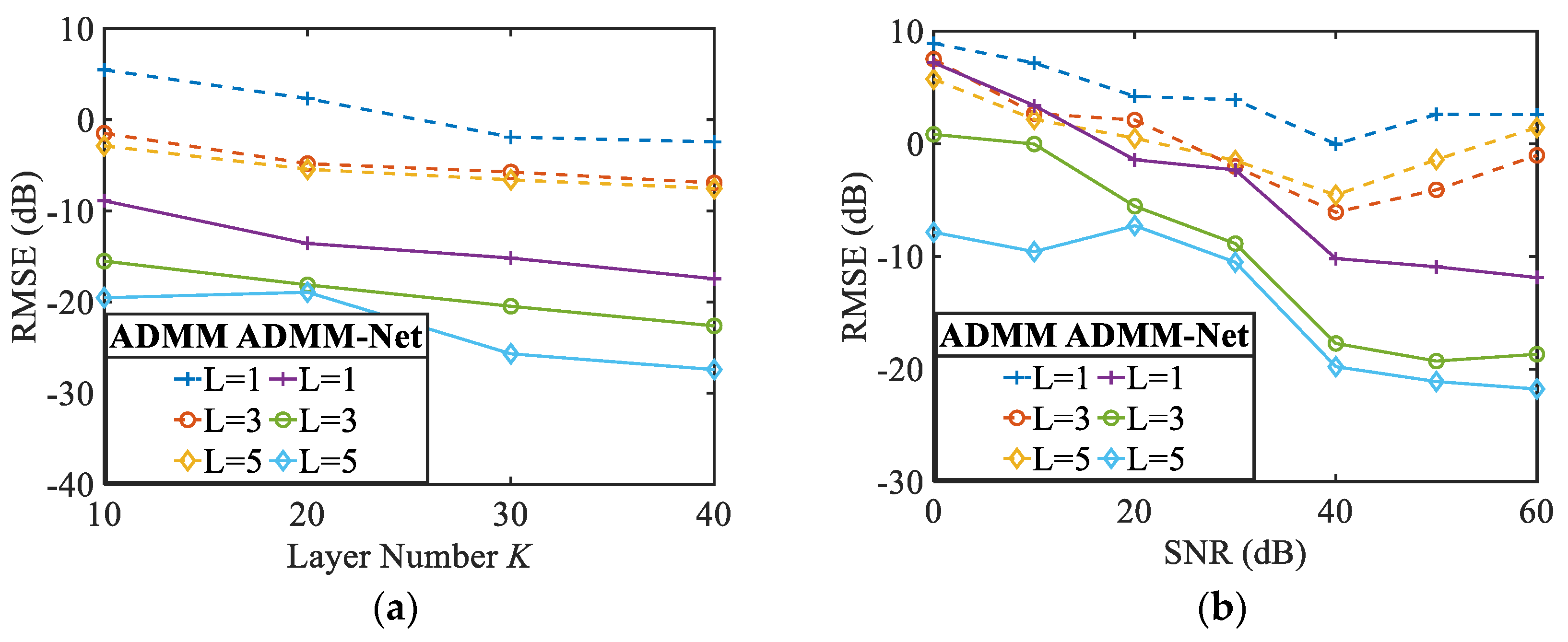Figure 4c shows that, as the number of network layers (the number of iterations) increases, the NMSEs of both ANM-ADMM-Net and ANM-ADMM algorithms gradually decrease, and the former is much smaller than the latter. In addition, only when the number of iterations of the ANM-ADMM algorithm is at least fifty to sixty times higher than the ANM-ADMM-Net, their NMSE is equal, which implies the computing complexity required for convergence is reduced.

The iteration parameters of DANM-ADMM algorithm are set as ${\rho }_0=0.1$, ${\lambda }_0=0.1$, and ${\gamma }_0=0.1$. Set different network layers $K=5~25$, initialize and train DANM-ADMM-Net (600 epochs), and the results are shown in Figure 5. Among them, Figure 5a,b is the training NMSEs and testing NMSEs of DANM-ADMM-Net when $K=5/10$, and Figure 5c shows the NMSEs of both when the number of network layers (iterations) $K=5~25$. Figure 5d reveals the NMSEs of algorithm when iterations $K=5~300$. Based on Figure 5a,b, the training and testing NMSEs of DANM-ADMM-Net decrease with the increase in training time and effectively reach convergence after 500 training epochs. In addition, Figure 5c shows that as the number of network layers (the number of iterations) increases, the NMSEs of both the DANM-ADMM-Net and DANM-ADMM algorithm decrease. However, the NMSE of the former is much smaller than that of the latter. From Figure 5c,d, the two have similar NMSE only when the number of iterations of the algorithm is fifty times higher than that of network when $K=10$. Therefore, it can be concluded that the proposed can learn the optimal iteration parameters from the constructed dataset and obtain better convergence performance.

In practical applications, the networks can be trained offline based on different simulation conditions to determine the range of network layers that can obtain better DOA estimation performance and lower computational complexity. Then, the network layers can be selected according to the actual situation.

4.2. DOA Estimation Results Analysis

4.2.1. 1D DOA Estimation Results Analysis

This subsection investigates the performance of ANM-ADMM-Net for DOA estimation and its upsides over the SBL algorithm, dual ANM, ANM-CVX and ANM-ADMM methods with simulation experiments. The root mean square error (RMSE) is evaluated by $M_c=100$ Monte Carlo trials.

$$\mathrm{RMSE}=\frac{1}{O}{\displaystyle \sum _{o=1}^O\sqrt{\frac{1}{K_t{M}_c}{\displaystyle \sum _{j=1}^{M_c}{\displaystyle \sum _{k_t=1}^{K_t}{({\widehat{\theta }}_{o,k_t}-{\theta }_{o,k_t})}^2}}}}$$

(35)

The results of different methods are shown in Figure 6, where grid numbers $N=100$, $K=200$ and $\lambda =1\mathrm{e}-3$ for the SBL algorithm [8]; $K=30$, $L=5$ for ANM-ADMM and ANM-ADMM-Net. The results indicate that unsuitable grid division inevitably causes the estimated DOA offset of the SBL algorithm. dual ANM and ANM-CVX methods are always the optimal estimation results. ANM-ADMM cannot recover the amplitude and degree of the signal perfectly due to limited iterations. However, the proposed ANM-ADMM-Net has a better estimation of amplitude and degree than the ANM-ADMM algorithm with fixed parameters, demonstrating the effectiveness of the combination of model-driven and data-driven DU methods.

Figure 7 shows the test RMSEs when the number of network layers $K=10~40$. The RMSEs of ANM-ADMM and ANM-ADMM-Net gradually decrease as the number of network layers increases (number of iterations), and the latter is much smaller than the former with fixed parameters. The above results demonstrate that the more layers of the network, the more optimal iterative parameters can be learned from the constructed dataset due to its powerful nonlinear fitting capability and superior flexibility, resulting in better DOA estimation performance. In other words, the DU-gridless DOA method based on ANM-ADMM-Net is suitable for efficiently resolving the different sparsity problems (different target signal problems) at a lower computational cost.

The testing dataset when SNR = 0~60dB is constructed to verify the noise robustness according to Section 3.2.2 (i.e., generate testing data for every SNR and noise regularization factor of dual ANM is 0.1), and the test results when $K=40$ are shown in Figure 7b. It can be seen that when $\mathrm{SNR}<20\mathrm{dB}$, ANM-ADMM is unable to be implemented for estimation. However, the proposed method still performs better under limited network layers/iterations, demonstrating the higher noise robustness of the latter with the optimal parameters. In addition, when $\mathrm{SNR}>40\mathrm{dB}$, the test RMSE of ANM-ADMM-Net tends to be stable and close to the results obtained in the noise-free case. The above implies that even if noise-free data train the network, the proposed method still obtains better parameter results and can perform DOA estimation for the actual array received data containing noise.

4.2.2. 2D DOA Estimation Results Analysis

This subsection investigates the performance of DANM-ADMM-Net for 2D DOA estimation and its upsides over the conventional 2D DOA methods with simulation experiments. The root mean square error (RMSE) is also evaluated by $M_c=100$ Monte Carlo trials.

$$\mathrm{RMSE}=\frac{1}{O}{\displaystyle \sum _{o=1}^O\sqrt{\frac{1}{K_t{M}_c}{\displaystyle \sum _{j=1}^{M_c}{\displaystyle \sum _{k_t=1}^{K_t}{({\widehat{\varphi }}_{o,k_t}-{\varphi }_{o,k_t})}^2+{({\widehat{\theta }}_{o,k_t}-{\theta }_{o,k_t})}^2}}}}$$

(36)

The 2D DOA results estimated by different methods when $M=20$, $K=20$ are shown in Figure 8, where the parameters of the 2D-MUSIC method are set to $\mathrm{SNR}=20\mathrm{dB}$, and the number of snapshots $L=20$. The results in Figure 8b show that the DANM-ADMM algorithm fails to precisely converge to the ground truth precisely at a finite number of iterations due to improper parameter settings, resulting in some deviations in both azimuth and pitch angles estimated for individual targets. In contrast, the parameters of the proposed method are optimized for data and networks, thus converging to a better result completely at a finite number of layers.

Figure 9a gives the results of the test RMSEs when the number of array elements $M=20$ and the number of network layers $K=5~25$. The RMSEs of DANM-ADMM and DANM-ADMM-Net gradually decrease as the number of network layers increases (number of iterations). When $K=25$, the RMSE of the latter is reduced by 20dB compared to the former with fixed parameters, which indicates that the more layers of the network, the more optimal iterative parameters can be learned from the constructed dataset, resulting in better 2D DOA estimation performance.

The test dataset is constructed by Section 3.4.3 when SNR = 0~60dB (i.e., test data are generated for each SNR) to verify the noise robustness of DANM-ADMM-Net. The results when $K=25$ are shown in Figure 9b. The tested RMSE of both methods decreased with increased SNR under a limited number of network layers/iterations. If we train the network with data when noise exists, for example, SNR = 10 dB, DANM-ADMM-Net performs better than DANM-ADMM under any circumstances. Therefore, to ensure higher noise robustness, one can estimate the signal-to-noise ratio first, and then use the corresponding data containing the noise to train the network.

4.3. Computational Complexity and Running Time Comparsion

This subsection analyzes the computational complexity and running time of SDPT3 based ANM-CVX method and ANM-ADMM-Net at different array elements when network layers $K=40$. The running time results when $M=10~50$, $L=5$ and $M=10$, $L=1~15$ are shown in Figure 10. The results of the comparison of DANM-CVX and DANM-ADMM-Net when network layers $K=25$ are also shown in Figure 11.

From the paper [43], it is known that the computational complexity of the solver SDPT3-based CVX method is $q_1^2{q}_2^2$, where $q_1$ denotes the number of variables and $q_2$ denotes the dimensionality of the SDP matrix. Therefore, the computational complexity of the CVX method for solving the ANM model is $O\{Q{(M+L)}^2{(ML+M+L)}^2\}$ and $O\{Q{(M+N)}^2{(MN+M+N)}^2\}$ for solving the DANM model. In contrast, while that of the ADMM method is $O\{Q{(M+L)}^3\}$ and $O\{Q{(M+N)}^3\}$, respectively, where $Q$ denotes the number of iterations, which indicates that when the matrix size is large, the computational complexity of the ANM-ADMM and DANM-ADMM methods to solve the ANM model and DANM model, respectively, is much smaller than that of the ANM-CVX and DANM-CVX methods, respectively.

It is important to emphasize that the computational complexity analysis of ANM/DANM-ADMM-Net in this paper does not include the computational costs required for network training, since it is possible to train offline and apply online. Moreover, after training to obtain the optimal parameters, the computational complexity of networks and its ADMM algorithms are identical and differ in the iterative parameters. Therefore, networks and ANM/DANM-ADMM algorithms will have the same computational complexity when applied with the same network layers (number of iterations). However, considering the reduced iterations requirements of networks, the computational complexity is further decreased compared to algorithms.

The results in Figure 10 show that the growth rate of the proposed method’s running time is much lower than that of the ANM-CVX and dual ANM methods, as the number of array elements or snapshots increases. In conclusion, ANM-ADMM-Net can be an alternative in the presence of larger-scale arrays or snapshots and high real-time requirements, and it is consistent with the above theoretical analysis. The same conclusion also can be drawn for DANM-CVX and DANM-ADMM-Net in Figure 11.

5. Conclusions

In this paper, a DU-based gridless DOA method is proposed. ANM-ADMM and DANM-ADMM algorithms are examined in the continuous domain, and the deep neural networks ANM-ADMM-Net and DANM-ADMM-Net are constructed for their problems. Their network structure, data set construction method, network initialization, and training method are introduced. Then, their performance is validated by simulation experiments. The results show that: compared with the existing methods, model-plus-data-driven ANM-ADMM-Net and DNM-ADMM-Net can learn the optimal iteration parameters from the data and quickly obtain more accurate 1D and 2D DOA estimation. The required computational complexity is reduced by 50~60 times and 20 times, respectively.