A Parallel Principal Skewness Analysis and Its Application in Radar Target Detection

Abstract

Radar is often affected by various clutter backgrounds in complex environments, so clutter suppression has important practical significance for radar target detection. The clutter suppression process conforms to the blind source separation (BSS) model. The principal skewness analysis (PSA) algorithm is a BSS algorithm with third-order statistics as the objective function, and its running speed is faster than the conventional BSS algorithm. Still, the PSA algorithm has the problem of error accumulation. This paper improves the PSA algorithm and proposes a parallel PSA (PPSA) algorithm. PPSA can estimate the directions corresponding to each independent component simultaneously and avoid the problem of error accumulation. PPSA uses parallel instead of serial computing, significantly improving the running speed. In this paper, the PPSA algorithm is applied to radar target detection. The simulation data and real data experiments verify the effectiveness and superiority of the PPSA algorithm in suppressing clutter.

1. Introduction

The moving targets of interest are often obscured by solid clutter and cannot be easily detected. Clutter suppression processing must be performed to improve the detection performance of the radar system for moving targets. There are many radar clutter suppression technologies, mainly multi-antenna cancellation technology [1,2,3,4,5], multi-dimensional domain filtering technology [6,7,8], dual-parameter constant false alarm rate detection technology [9], etc. Space-time adaptive processing (STAP) is a technique to distinguish moving objects and clutter from space-time two-dimensional, and it can effectively suppress clutter [10], so it is widely used. However, the traditional STAP method usually needs to select a certain number of range unit echo data around the unit to be detected as training samples. According to the well-known RMB criterion [9], to obtain the clutter suppression performance with an average performance loss of no more than 3dB relative to the optimal processing, it requires at least twice the system degrees of freedom of IID training samples. However, the number of samples obtained in actual radar operating scenarios is usually less than twice the system degrees of freedom, so this will seriously reduce the clutter suppression effect.

To solve the problem of insufficient training samples, Qian et al. applied the blind source separation (BBS) algorithm to clutter suppression [11]. The radar echo signal can be regarded as a linear combination of target echo and clutter echo [12]. Clutter suppression separates the radar target signal from the mixed data, a process that conforms to the BSS model [13]. Since the clutter signal and the target signal are independent, the BSS method can be used to distinguish the target signal and the clutter signal.

In the research field of BSS, independent component analysis (ICA) has become a critical signal-processing method in recent years. ICA is a higher-order statistical data analysis that seeks to maximize non-Gaussian quantities to separate independent signal sources [14]. Heranlt and Jutten first proposed the idea in 1986. FastICA is an improved algorithm of ICA, which can select indicators such as skewness, negentropy, and kurtosis as non-Gaussian metrics [15]. The FastICA algorithm can achieve three times the convergence speed, which is better than most commonly used ICA algorithms [16]. However, each iteration of FastICA needs to involve all pixels to find the optimal projection direction, which is time-consuming when dealing with high-dimensional data. To solve this problem, Geng [17] proposed a principal skewness analysis (PSA) method. PSA can be thought of as a third-order generalization of PCA. Meanwhile, it is also equivalent to FastICA when choosing skewness as the non-Gaussian metric. On this basis, Geng et al. further proposed momentum PSA (MPSA) [18] and principal kurtosis analysis (PKA) [19]. PSA and MPSA use the orthogonal complement strategy in the solution process, but supersymmetric tensors do not have natural orthogonality [20]. Thus, except for the first eigenpair, all other solutions obtained by PSA inevitably deviate from the exact eigenpair of the co-skewness tensor. To alleviate this problem, Geng et al. [21] proposed a new non-orthogonal PSA (NPSA) algorithm. NPSA offers a unique search strategy by introducing the Kronecker product, which can search for solutions in a larger space and obtain more precise solutions for each eigenpair. Unfortunately, the NPSA algorithm still obtains approximate solutions of eigenpairs.

Regarding the issue above, this paper proposes a new parallel principle of skewness analysis (PPSA) algorithm. Different from the random initialization of the existing PSA algorithm, PPSA uses the eigenvector of the co-skewness tensor slice as the initial value. Unlike the existing PSA algorithm that imposes constraints and solves each eigenpair in turn, PPSA no longer imposes restrictions and solves each eigenpair in parallel. Compared with the existing PSA method, which can only obtain approximate solutions, the PPSA algorithm can accurately obtain real solutions.

Finally, this paper applies the PPSA algorithm to radar target detection. The PPSA algorithm uses the skewness value to decompose the radar echo to separate radar clutter and target. We compared our method to other well-known methods in the literature to demonstrate its superiority. The signal-to-noise ratio (SNR) in simulation datasets and visual results in real datasets are used to demonstrate the performance analysis. The experimental results show that the PPSA method is superior.

2. Background

2.1. Preliminaries

Following [22], an Nth-order tensor is defined as $\mathfrak{R}\in {ℝ}^{I_1\times I_2\times \dots I_N}$, where is the order of $\mathfrak{R}$, also called the way or mode. For $N$ = 1, it is a vector. For $N$ = 2, it is a matrix. For $N\ge 3$, it is a higher order tensor. The element of $\mathfrak{R}$ is denoted by $R_{i_1,i_2,\dots i_N}$, $i_N\in \{1,2,\dots ,I_n\},1\le n\le N$. Fibers, the higher-order analogue of matrix rows and columns, are defined by fixing every index except one. Slices are two-dimensional sections of a tensor, defined by fixing all except two indices. For a third-order tensor $\mathfrak{R}\in {ℝ}^{I_1\times I_2\times I_3}$, as shown in Figure 1, its three different slices are called horizontal, lateral and frontal slices, which can be denoted by $R_{i::}$, $R_{:j:}$, and $R_{::k}$, respectively. A tensor is called supersymmetric if its elements remain invariant under any permutation of the indices. The co-skewness tensor is supersymmetric.

2.2. PSA Algorithm

In the PSA algorithm, the co-skewness tensor is constructed, similar to constructing the covariance matrix in PCA, to calculate the skewness of the image in the direction. We assume that the image dataset is $\mathit{X}=[{\mathit{x}}_1,{\mathit{x}}_{i2},\dots ,{\mathit{x}}_{iN}]\in {\mathit{R}}^{L\times N}$, where ${\mathit{x}}_i$ is the $L\times 1$ vector and $N$ is the number of pixels. The image should first be centered and whitened by $\mathit{R}={\mathit{F}}^{\mathrm{T}}(\mathit{X}-\mathit{m})$, where $\mathit{m}=(1/N){\displaystyle {\sum }_{i=1}^N{\mathit{x}}_i}$ is the mean vector and $\mathit{R}=[{\mathit{r}}_1,{\mathit{r}}_2,\cdots ,{\mathit{r}}_N]$ is the whitened image. $\mathit{F}=\mathit{E}{\mathit{D}}^{-0.5}$ is called the whitening operator, where $\mathit{E}$ is the eigenvector matrix of the covariance matrix, and $\mathit{D}$ is the corresponding eigenvalue diagonal matrix. Then, the co-skewness tensor is calculated by the following formula:

$$\mathit{S}=\frac{1}{N}{\displaystyle \sum _{i=1}^N\mathit{r}\circ \mathit{r}\circ \mathit{r}}$$

(1)

The above formula “◦” represents the outer product of two vectors. Clearly, $\mathit{S}$ is a supersymmetric tensor with a size of $L\times L\times L$. Then, the skewness of the image in any direction $\mathit{u}$ can be calculated by the following formula:

$$\mathrm{skew}(\mathit{u})=\mathit{S}{\times }_1\mathit{u}{\times }_2\mathit{u}{\times }_3\mathit{u}$$

(2)

where $\mathit{u}\in {\mathit{R}}^{L\times 1}$ is a unit vector, i.e., ${\mathit{u}}^{\mathrm{T}}\mathit{u}=1$. So the optimized model is the following:

$$\{\begin{array}{l}\underset{\mathit{u}}{\max }\hspace{1em}\hspace{1em}\mathit{S}{\times }_1\mathit{u}{\times }_2\mathit{u}{\times }_3\mathit{u}\\ s.t.\hspace{1em}\hspace{1em}{\mathit{u}}^{\mathrm{T}}\mathit{u}=1.\end{array}$$

(3)

Solving the above equation using the Lagrangian method:

$$\mathit{S}{\times }_1\mathit{u}{\times }_3\mathit{u}=\lambda \mathit{u}$$

(4)

Using the fixed-point method to calculate each $\mathit{u}$ for each unit, which can be expressed as follows:

$$\{\begin{array}{l}\mathit{u}=\mathit{S}{\times }_1\mathit{u}{\times }_3\mathit{u}\\ \mathit{u}=\mathit{u}/{\Vert \mathit{u}\Vert }_2\end{array}$$

(5)

If it has a fixed point, the solution $\mathit{u}$ is called the first principal skewness direction and $\lambda$ is its skewness. Likewise, $(\lambda ,\mathit{u})$ is also called the eigenvalue/eigenvector pair of a tensor, introduced by Lim [23] and Qi [24].

To prevent the second eigenvector from converging to the same eigenvector, the algorithm generates a new tensor calculation in the orthogonal complement space of $\mathit{u}$.

$$\mathit{S}=\mathit{S}{\times }_1{\mathit{P}}_u^{\perp }{\times }_2{\mathit{P}}_u^{\perp }{\times }_3{\mathit{P}}_u^{\perp }$$

(6)

where ${\mathit{P}}_u^{\perp }=\mathit{I}-\mathit{u}{({\mathit{u}}^{\mathrm{T}}\mathit{u})}^{-1}{\mathit{u}}^{\mathrm{T}}$ is the orthogonal complement projection operator of $\mathit{u}$ and $\mathit{I}$ is the $L\times L$ identity matrix.

Then, the same iterative method is used for the new tensor $\mathit{S}$ to obtain the second eigenvector, and the following process is also carried out in the same way until $L$ eigenpairs are obtained.

3. Parallel PSA Algorithm

3.1. Limitations of Existing PSA Algorithms

The existing PSA algorithm initialization adopts random generation of the initial value, which means that given different initialization, it may converge to other solutions (eigenpairs) [25]. And the existing PSA algorithm can only obtain the approximate solutions of eigenpairs.

We give a simple example here to illustrate these two phenomena more intuitively. Consider a supersymmetric tensor $\mathit{S}\in {ℝ}^{2\times 2\times 2}$, whose two frontal slices are as follows:

$${\mathit{S}}_1=\left[\begin{array}{cc}2& -1\\ -1& 0.8\end{array}\right],{\mathit{S}}_2=\left[\begin{array}{cc}-1& 0.8\\ 0.8& 0.3\end{array}\right]$$

Eventually, the obtained two eigenvectors are the following:

$${\mathit{u}}_1={\left[0.8812,-0.4727\right]}^{\mathrm{T}},{\mathit{u}}_2={[0.3757,0.9267]}^{\mathrm{T}}$$

and their inner product is ${\mathit{u}}_1^{\mathrm{T}}{\mathit{u}}_2=-0.1070$, which means that they are nonorthogonal.

However, when using the PSA and MPSA methods to solve when the initial value is closer to ${\mathit{u}}_1$, it will first converge to ${\mathit{u}}_1^{\mathrm{PSA}}$, and then generate the initial value ${\mathit{u}}_2^{\mathrm{PSA}}$, according to the orthogonal constraint principle. The final convergence result is the following:

$${\mathit{u}}_1^{\mathrm{PSA}}={[0.8812,-0.4727]}^{\mathrm{T}},{\mathit{u}}_2^{\mathrm{PSA}}={[0.4727,0.8812]}^{\mathrm{T}}$$

When the initial value is closer to ${\mathit{u}}_2$, it will first converge to ${\mathit{u}}_2^{\mathrm{PSA}}$, and then generate the initial value ${\mathit{u}}_1^{\mathrm{PSA}}$, according to the principle of orthogonal constraints. The final convergence result is the following:

$${\mathit{u}}_1^{\mathrm{PSA}}={[0.3756,0.9268]}^{\mathrm{T}},{\mathit{u}}_2^{\mathrm{PSA}}={[0.9268,-0.3756]}^{\mathrm{T}}$$

The above results are shown in Figure 2.

When using the NPSA methods to solve, when the initial value is closer to ${\mathit{u}}_1$, the results obtained by the NPSA algorithm are the following:

$${\mathit{u}}_1^{\mathrm{NPSA}}={[0.8812,-0.4727]}^{\mathrm{T}},{\mathit{u}}_2^{\mathrm{NPSA}}={[0.3351,0.9422]}^{\mathrm{T}}$$

When the initial value is closer to ${\mathit{u}}_2$, the results obtained by the NPSA algorithm are the following:

$${\mathit{u}}_1^{\mathrm{NPSA}}={[0.3756,0.9268]}^{\mathrm{T}},{\mathit{u}}_2^{\mathrm{NPSA}}={[0.8799,-0.4752]}^{\mathrm{T}}$$

The above results are shown in Figure 3.

This simple example intuitively illustrates that the existing PSA algorithm cannot accurately obtain the actual eigenpairs of the co-skewness tensors. It is also demonstrated that existing PSA algorithms randomly generate initial values, converging to different eigenpair for each run. What is more, these problems will become more obvious as the tensor dimension increases. The solution of a 3-order 2-dimensional supersymmetric tensor may connect to two different eigenpairs. However, the solution of a 3-order n-dimensional supersymmetric tensor may obtain $n!$ different eigenpairs. Computational errors arising from solving eigenpairs will accumulate in subsequent eigenpair computations, and this will cause computational errors to increase as the order of computation increases. Therefore, designing an accurate and stable method for calculating and solving is very important.

3.2. PPSA

Regarding the issue above, this paper improves the PSA algorithm and proposes a high-precision PPSA algorithm. PPSA uses the eigenvector of the co-skewness tensor slice as the initial value, which avoids the problem of different results each time caused by random initialization. PPSA uses parallel computing instead of serial computing, which avoids the problem of error accumulation.

Solving the actual eigenpair of the co-skewness tensor can be understood as solving the local maximum value solution of the tensor [25]. When we use the fixed-point iterative method to solve, as long as the initial value falls in each convergence region of the co-skewness tensor, we can obtain all maximal solutions accurately. Therefore, the problem of solving the eigenpair of the co-skewness tensor can be transformed into the problem of initial value selection. Standard initialization methods include random initialization and random initialization based on orthogonal constraints. Although methods of random initialization can be solved accurately, they are greatly affected by the initial value and are not repeatable. Therefore, it is crucial to design a method that can repeat the initial value and solve the eigenpair of the co-skewness tensor stably and accurately.

The PPSA algorithm fully considers the data structures and selects the eigenvector of the slice of the co-skewness tensor as the initial value of the iteration. First, this method is repeatable. Second, this approach is parallel because co-skewness tensor slices are real symmetric matrices. The eigenvectors corresponding to different eigenvalues of the symmetric matrix are orthogonal to each other. At last, this method produces a stable and accurate solution compared to the orthogonal random initialization method because we believe it will provide an initial guess around the optimal solution.

Next, we briefly prove this conjecture. Suppose $\mathit{S}\in {ℝ}^{[3,n]}$, if $\lambda$ is an eigenvalue of the co-skewness tensor $\mathit{S}$, let $\mathit{u}$ be the unit eigenvector of $\mathit{S}$ with respect to $\lambda$, $\mathit{u}={[a_1,a_2,\cdots ,a_n]}^{\mathrm{T}}$, and ${\mathit{u}}^{\mathrm{T}}\mathit{u}=1$. Solving $\mathit{S}{\times }_1\mathit{u}{\times }_3\mathit{u}=\lambda \mathit{u}$, it is equivalent to solve the following formula:

$$\{\begin{array}{l}{\mathit{u}}^{\mathrm{T}}\times {\mathit{S}}_{::1}\times \mathit{u}=\lambda a_1\\ {\mathit{u}}^{\mathrm{T}}\times {\mathit{S}}_{::2}\times \mathit{u}=\lambda a_2\\ ⋮\hspace{1em}\hspace{1em}⋮\hspace{1em}\hspace{1em}⋮ =\hspace{1em}⋮\\ {\mathit{u}}^{\mathrm{T}}\times {\mathit{S}}_{::n}\times \mathit{u}=\lambda a_n\end{array}$$

(7)

From Equation (7), it can be known that solving the local extremum solution of the co-skewness tensor is equivalent to finding the maxima and minima jointly by multiple principal component analyses. Taking the eigenvector of the slice of the co-skewness tensor as the initial value of the iteration can be understood as approximating the extreme point of the joint principal component from the extreme point of a single principal component. Therefore, the initial value generated by this initialization method is closer to the actual eigenpair than randomly selecting the initial value.

For convenience, the pseudo-code of PPSA is summarized in Algorithm 1.

Algorithm 1 PPSA

Input: Input data $\mathit{R}\in {\mathit{R}}^{L\times N}$.

Output: output transformation matrix $\mathit{U}$, $\mathit{Y}={\mathit{U}}^{\mathrm{T}}\tilde{\mathit{R}}$.

1: whiten the data to obtain $\tilde{\mathit{R}}$.

2: calculate the co-skewness tensor $\mathit{S}$ according to (1).

3: calculate all eigenvectors of slices of tensor (${\mathit{S}}_{1::}$), denoted as $\mathit{V}$

% main loop: %

4: $\mathrm{for} i=1:L \mathrm{do}$

5: k = 0

6: ${\mathit{u}}_i^{(k)}=\mathit{V}(:,i)$

7: while stop conditions are not meet do

8:  ${\mathit{u}}_i^{(k+1)}=\mathit{S}{\times }_1{\mathit{u}}_i^{(k+1)}{\times }_3{\mathit{u}}_i^{(k+1)}$

9:  ${\mathit{u}}_i^{(k+1)}={\mathit{u}}_i^{(k+1)}/{\Vert {\mathit{u}}_i^{(k+1)}\Vert }_2$

10: end while

11: ${\mathit{U}}_{:i}={\mathit{u}}_i^{(k+1)}$

12: end for

% output %

13: $\mathit{Y}={\mathit{U}}^{\mathrm{T}}\tilde{\mathit{R}}$;//$\mathit{U}$ is the final principal skewness transformation matrix, and $\mathit{Y}$ is the transformed image.

It should be noted that the loop termination condition in step 7 in the PPSA algorithm includes the minimum allowable error $\mathit{\epsilon }$ and the maximum number of loops $\mathit{K}$. In this paper, $\mathit{\epsilon }$ is set to 0.0001, and $\mathit{K}$ is set to 1000. $\mathit{U}$ is the final non-orthogonal principal skewness transformation matrix.

Also calculate the example in the above Section 3.1, repeat the above operation with the PPSA algorithm, and the results obtained are the following:

$${\mathit{u}}_1^{\mathrm{PPSA}}={[0.8812,-0.4727]}^{\mathrm{T}},{\mathit{u}}_2^{\mathrm{PPSA}}={[0.3756,0.9268]}^{\mathrm{T}}$$

As shown in Figure 4, it is obvious that the results obtained by PPSA are almost perfectly coincident with the actual eigenpairs ${\mathit{u}}_1$, ${\mathit{u}}_2$, and the solution results are unique.

3.3. Complexity Analysis

This section theoretically compares the computational complexity of the PSA algorithm and the PPSA algorithm. The difference between the PPSA and the PSA algorithm is the order of orthogonalization. PSA is solved iteratively first, and then the orthogonal constraints are imposed. The PPSA algorithm is orthogonalized first and then solved iteratively. Since the basic process of both methods is the same, only the computational complexity of the primary loop solution needs to be considered. For data of size $L\times M$, the PSA algorithm only needs to loop $L$ times. Assuming that each loop requires $K$ iterations, where $K$ is the average number of iterations, the PSA algorithm must perform $KL$ operations. Similarly, for data of size $L\times M$, the PPSA algorithm only needs to loop $L$ times, assuming that each loop needs to iterate $H$ times, so the PPSA algorithm eventually needs $HL$ operations, generally $H\le K$. Although the algorithm complexity of PPSA is at the same level as that of PSA, the main advantage of the PPSA algorithm over the PSA algorithm is that the PPSA algorithm is parallel, so it can use parallel computing to improve the running speed. It can be seen from the running speed comparison experiments that when processing high-dimensional data, the PPSA algorithm runs faster after parallel accelerated calculation.

4. Experiment

In this paper, the PPSA algorithm is applied to blind image separation (BIS) and radar target detection, and a comparative experiment is carried out with several classical methods. All algorithms are completed on a laptop with CPU AMD Ryzen 7 5800H, 16 GB RAM, @3.20 GHz, and all programs are programmed and implemented on MATLAB R2021a.

4.1. Experiment 1: Blind Image Separation

In this paper, the PPSA algorithm is firstly applied to the problem of blind image separation (BIS). The purpose of BIS is to estimate the mixing matrix, denoted as $\mathit{B}$. To evaluate the separation performance of the PPSA algorithm, we compare it with algorithms such as FastICA [15], PSA [17], MPSA [18], NPSA [21], and MSDP [25]. In this experiment, this paper selects $n$ grayscale images with a size of 256 × 256 pixels as the source image, where $n$ is 2~6 respectively. Since the real source image is known, we can compare it with the results obtained by each algorithm. Due to space limitations, we did not show all the experimental results, but only selected the case of $n=3$ for display. The results are shown in Figure 5. To ensure the reliability of the conclusions, we also conducted two other combinations of experiments, in each combination we randomly selected three different source images for the experiments.

From the experimental results, all the above algorithms can separate the source image from the mixed image. In order to quantitatively evaluate the performance of the above six algorithms, we use five evaluation indicators to evaluate the separation results obtained by the above six algorithms. The five evaluation indicators are intersymbol interference (ISI) [21], total mean square error (TMSE) [21], correlation coefficient ($\rho$) [21], peak signal-to-noise ratio (PSNR) [21] and running time (T). It is worth noting that except for the PPSA algorithm and the MSDP algorithm, the results obtained by the other four algorithms are random, so we take the average of 10 runs as the final result.

Table 1. Comparison of FastICA, PSA, MPSA, NPSA, MSDP and PPSA for the index of five different combinations. An average result of the runs is computed.

	Index	FastICA	PSA	MPSA	NPSA	MSDP	PPSA
1	ISI	0.6757	0.0681	0.0551	0.0253	0.0203	0.0203
	TMSE	3.2856 × 10−11	2.5547 × 10−11	2.5548 × 10−11	3.8168 × 10−11	1.8645 × 10−11	1.8645 × 10−11
	$\rho$	0.9544 0.9889 0.9968	0.9954 0.9992 1.0000	0.9954 0.9988 1.0000	0.9992 0.99997 1.0000	0.9998 0.9992 1.0000	0.9998 0.9992 1.0000
	PSNR/dB	66.1696 70.0325 79.2579	76.6105 72.6448 90.9901	77.7449 73.7954 90.4324	83.6350 74.4358 91.1667	85.9129 74.4870 91.3285	85.9129 74.4870 91.3285
	T/s	0.0042	0.0011	0.0010	0.0043	2.8594	0.0009
2	ISI	0.4844	0.1442	0.1524	0.0787	0.0745	0.0745
	TMSE	3.2241 × 10−11	2.6798 × 10−11	2.6337 × 10−11	2.5154 × 10−11	1.9555 × 10−14	1.9555 × 10−14
	$\rho$	0.9749 0.9900 0.9970	0.9967 0.9905 0.9999	0.9967 0.9907 0.9998	0.9995 0.9920 1.0000	0.9997 0.9921 1.0000	0.9997 0.9921 1.0000
	PSNR/dB	69.1886 73.7143 76.9175	74.9389 73.1186 89.0466	75.6708 74.3531 90.4683	83.4588 70.1218 94.0776	83.7674 70.6017 94.7823	83.7674 70.6017 94.7823
	T/s	0.0052	0.0011	0.0010	0.0042	3.1046	0.0008
3	ISI	0.2965	0.0405	0.0452	0.0041	0.0006	0.0006
	TMSE	2.6603 × 10−10	2.6628 × 10−10	1.9986 × 10−10	3.4050 × 10−10	1.7480 × 10−10	1.7480 × 10−10
	$\rho$	0.9756 0.9950 0.9969	0.9966 0.9994 0.9998	0.9962 0.9995 0.9999	0.9997 1.0000 1.0000	1.0000 1.0000 1.0000	1.0000 1.0000 1.0000
	PSNR/dB	69.9228 61.8123 82.3327	83.2559 61.1492 87.5416	78.8206 58.8872 90.4749	91.4669 61.2297 94.0424	96.6388 64.0212 95.1910	96.6388 64.0212 95.1910
	T/s	0.0048	0.0012	0.0009	0.0033	2.9786	0.0007

shows the ISI, TMSE, $\rho$, PSNR, and T of the six algorithms under three different combinations in detail. For the ISI, TMSE, and T, the smaller the index value, the better the algorithm performs; for the $\rho$ and PSNR, the larger the index value, the better the algorithm performs [21]. From Table 1, it can be found that the results obtained by the PPSA and MSDP algorithms are entirely consistent. Because the MSDP algorithm can accurately obtain the eigenpair of the tensor [25], this shows that the PPSA algorithm can also accurately obtain the actual solution. The PPSA and MSDP algorithms have the smallest ISI and TMSE in all the combinations. It can also be seen that PPSA has the smallest T in all the combinations. And compared with the other four algorithms, the $\rho$ and PSNR obtained by the PPSA algorithm also have advantages in all combinations.

Finally, combined with the comparison results of several indices, it shows that the PPSA algorithm has more accurate and robust performance in BIS applications.

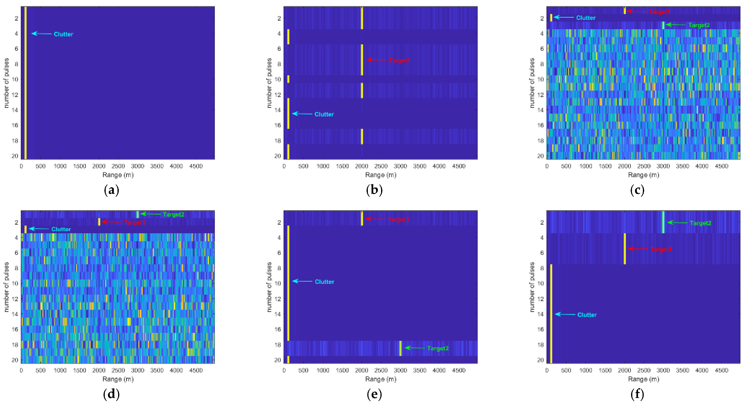
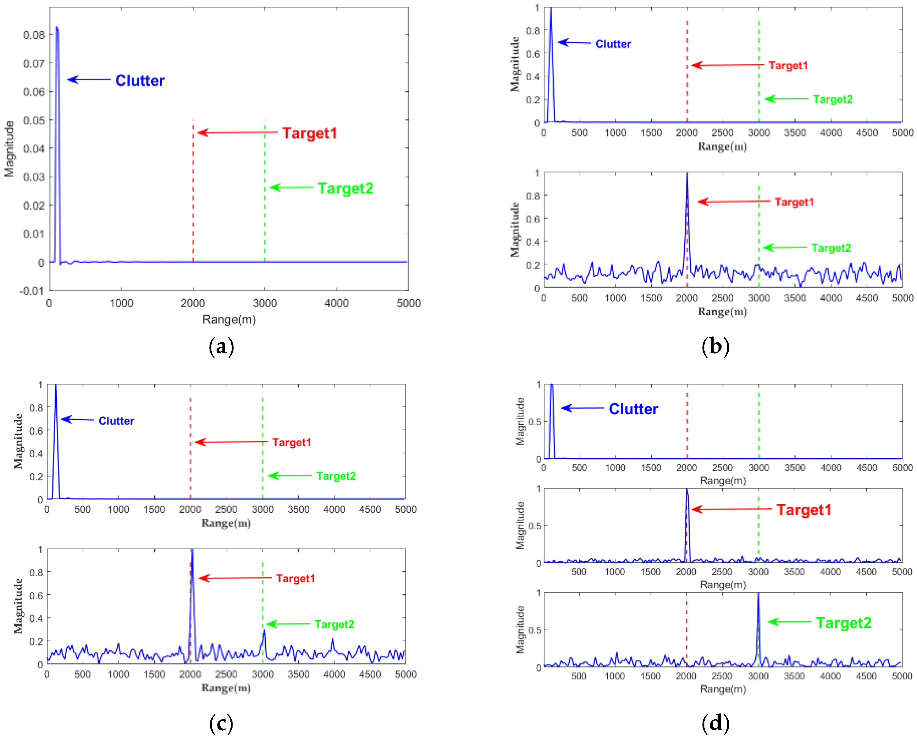
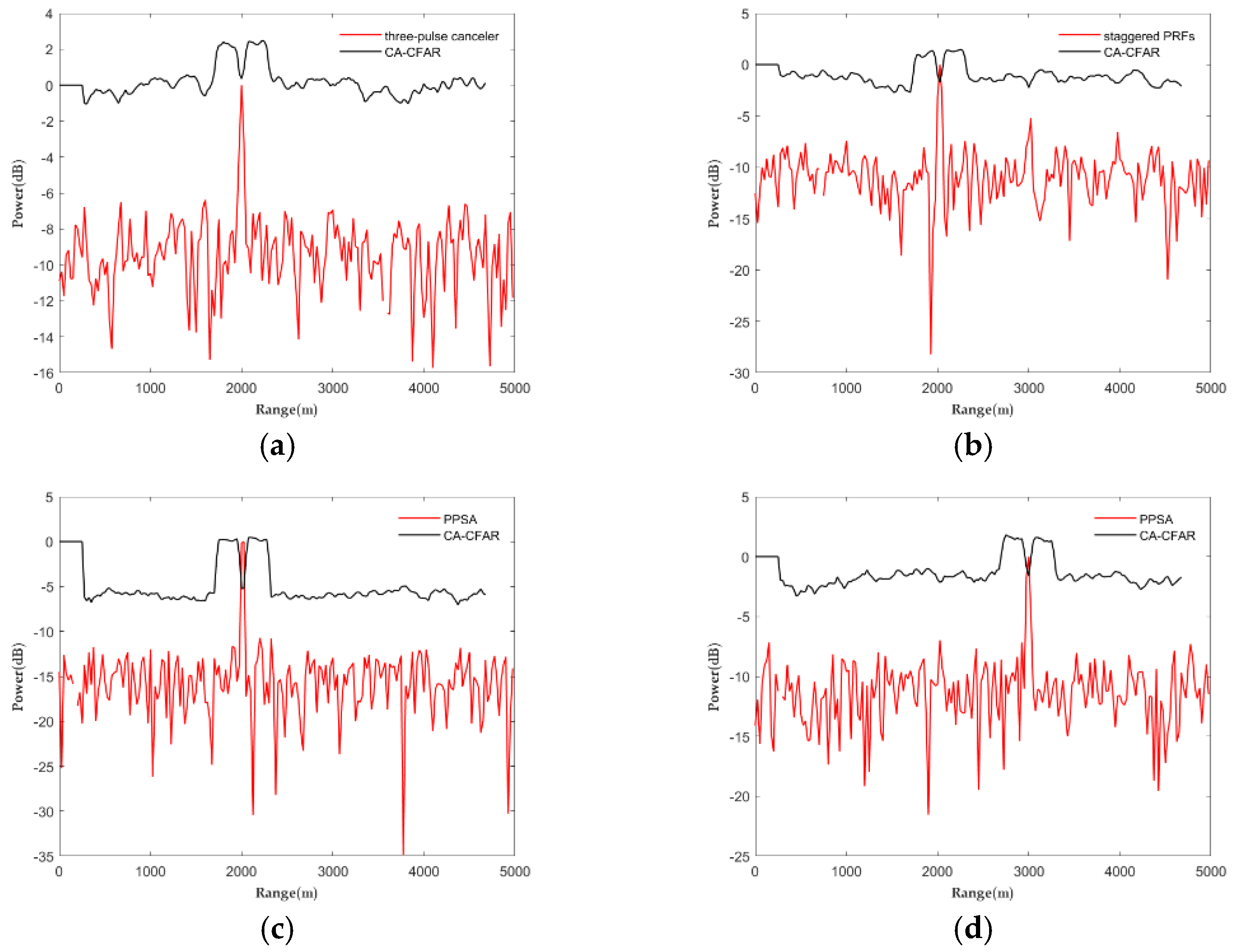
4.2. Experiment 2: Moving Target Detection under Low SNR

In this section, firstly, we apply the PPSA algorithm to moving object detection under a low SNR. This section uses a simulation dataset to verify the effect of the PPSA algorithm on noise suppression. We compared the PPSA algorithm with incoherent accumulation, coherent accumulation, FastICA [15], PSA [17], MPSA [18], and NPSA [21]. Quantitative and visual results are compared.

The simulation data set experiment is as follows. We generate radar echo data according to the radar system parameters given in

Table 2. Radar system parameters.

Parameter	Numerical Value
pulse repetition frequency/Hz	30,000
radar wavelength/m	0.03
Pulse train length	200
Radar operating frequency range/GHz	5~15
Antenna height/m	100
bandwidth	3 M
Sampling Rate	6 M
Receiver gain/dB	20
Noise figure/dB	0

and generate targets according to the target parameters in

Table 3. Movement target parameters.

Parameter	Target 1	Target 2
distance/m	2024.66	3518.63
radar cross section/m2	1.00	1.00
radial velocity/m/s	30	60

. We simulate 30 received pulse echoes for the previously defined radar and target. Figure 6a shows the original signal of the simulation, and Figure 6b–f are the results after noise suppression by algorithms such as FastICA, PSA, MPSA, NPSA, and PPSA, respectively.

From Figure 6a, we find that target 1 is visible, while target 2 is overwhelmed by noise. From Figure 6b–d, we can see that FastICA, PSA, and MPSA can separate the targets, but there are many interferences in their obtained results. From Figure 6e,f, we can see that NPSA and PPSA can effectively and accurately separate target 1 and target 2, and the separation effect of the PPSA algorithm is better.

Different from the existing PSA algorithm that solves each eigenpair in sequence, the PPSA algorithm can solve each eigenpair in parallel, so the PPSA algorithm can use Parfor to accelerate the calculation in parallel. We will use Parfor’s PPSA algorithm for parallel accelerated computing named FastPPSA. The principle of FastPPSA is the same as that of the PPSA algorithm, except that FastPPSA adopts Parfar parallel acceleration. We then compared the running times of the above algorithms, and the evaluation times are shown in

Table 4. Running time evaluation of BSS Algorithm.

Method	FastICA	PSA	MPSA	NPSA	PPSA	FastPPSA
Time (s)	1.5076	5.9706	5.8058	7.9262	5.7963	0.8143

.

Table 4 shows that the FastPPSA algorithm is superior to other BSS algorithms in terms of computational efficiency.

Then, we compare the PPSA algorithm with traditional incoherent and coherent accumulation algorithms. The results are shown in Figure 7. Figure 7a shows the original signal of the simulation, and Figure 7b–d are the results of incoherent accumulation, coherent accumulation, and the PPSA algorithm, respectively.

As shown in Figure 7, it can be seen that the above methods can effectively suppress the noise. In order to objectively and quantitatively evaluate the performance of each algorithm, the radar echo’s target SNR is defined as the ratio of the amplitude of the target signal to the mean value of the echo amplitude of the surrounding area. The quantitative results are shown in

Table 5. SNR comparison of target 1.

Method	Target 1 Echo Amplitude	Mean Noise Amplitude	SNR/dB
original signal	1.0000	0.1238	18.1456
noncoherent	1.0000	0.0601	24.4225
coherent	1.0000	0.0291	30.7221
PPSA	1.0000	0.0237	32.5050

and

Table 6. SNR comparison of target 2.

Method	Target 2 Echo Amplitude	Mean Noise Amplitude	SNR/dB
original signal	0.3040	0.1238	7.8031
noncoherent	0.2801	0.0601	13.3688
coherent	0.3351	0.0291	21.2256
PPSA	1.0000	0.0687	23.2609

.

Table 5 and Table 6 show that the PPSA algorithm obtains the highest SNR result, and the SNR has been significantly improved compared with the original signal.

To intuitively evaluate the clutter effect of the above algorithms, we perform CFAR detection on the results processed by each algorithm. In the simulation experiments in this paper, the unit average CFAR is used, the false alarm probability is (10⁻³), the protection unit is 2, and the reference unit is 10. The target detection results are shown in Figure 8.

The detection performance of objects is shown in Figure 8. It can be seen that the incoherent accumulation and coherent accumulation can only detect target 1 but cannot effectively detect target 2.

In contrast, the PPSA algorithm can effectively detect two moving targets, so the noise suppression performance of PPSA is better than that of incoherent and Coherent accumulation.

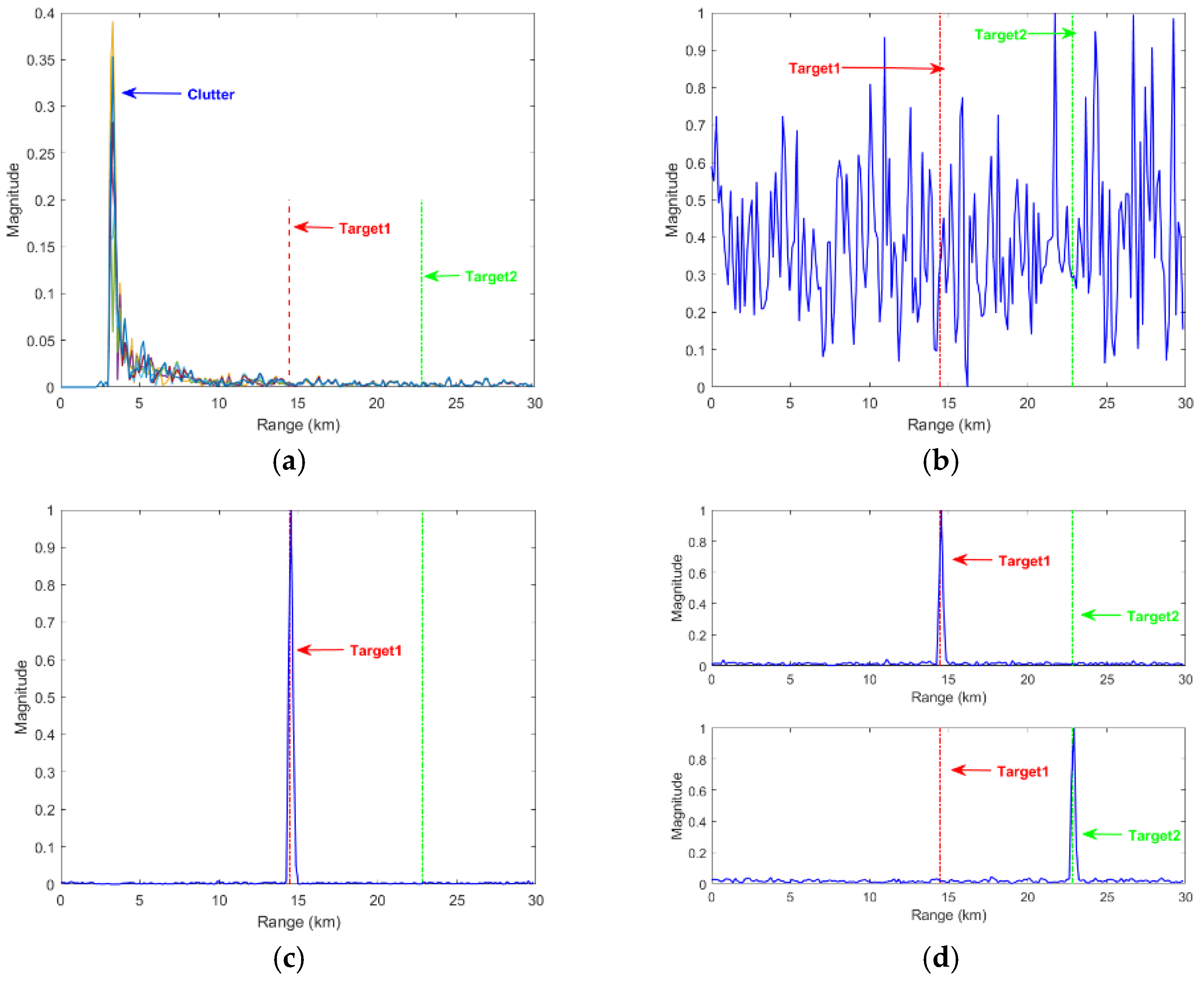
4.3. Experiment 2: Single-Channel Complex Background Micro-Moving Target Detection

This section applies the PPSA algorithm to detect tiny moving objects in a complex single-channel background. In this section, we also use the simulation data set to verify the effect of the PPSA algorithm on clutter suppression. We compared the PPSA algorithm with three-pulse canceler(TPC) [7], staggered pulse canceler(SPC) [7], FastICA [15], PSA [17], MPSA [18], and NPSA [21]. Quantitative and visual results were compared.

The simulation data set experiment is as follows. In this paper, radar echo data is generated according to the radar system parameters given in Table 2, and moving targets are generated according to the moving target parameters in

Table 7. Movement target parameters.

Parameter	Sports Goal 1	Sports Goal 2
distance/m	2000	3000
radar cross section/m2	1	1
radial velocity/m/s	−80	blind speed

. It is important to note that we set the speed of target 2 as a blind speed. We set the Doppler signature of the target with the pulse repetition frequency, a setting that prevents the MTI radar from detecting the target. The clutter signal was generated using the simplest clutter model (constant gamma model) with the gamma value set to −20 dB. This gamma value is typical of flat ground clutter. Finally, we simulated 20 pulse echoes using the above radar system parameters and moving target parameters. Figure 9a shows the original signal of the simulation, and Figure 9b–f show the results of algorithms such as FastICA, PSA, MPSA, NPSA, and PPSA, respectively.

As shown in Figure 9a, the clutter is visible, and the clutter completely submerges the target signal. From Figure 9b–d, it can be seen that FastICA, PSA, and MPSA can separate the targets, but they have many interferences. Additionally, their solutions are affected by random initial values, resulting in different results for each run. From Figure 9e,f, NPSA and PPSA can effectively and accurately separate target 1 and target 2.

Then we compare the running time of the above algorithms, and the evaluation time is shown in

Table 8. Running time evaluation of BSS Algorithm.

Method	FastICA	PSA	MPSA	NPSA	PPSA	FastPPSA
Time (s)	0.7189	1.6342	1.5340	1.7045	1.5023	0.2196

.

Table 8 shows that the FastPPSA method has advantages over the other algorithms mentioned above in terms of running time.

We then compare the PPSA algorithm with the traditional three-pulse and staggered pulse canceler. The results are shown in Figure 10. Figure 10a shows the original signal of the simulation, and Figure 10b–d are the results of three-pulse canceler, staggered pulse canceler, and PPSA, respectively.

Figure 10b shows that after the three-pulse canceler, a peak appears at target 1, and there is no obvious peak at target 2. From Figure 10c,d, it can be seen that the clutter is effectively suppressed, and there are obvious peaks where the two targets are located.

In many cases, the primary interference affecting radar detection performance is not noise but clutter. Therefore, the signal-to-clutter ratio (SCR) is often more critical than the SNR. To objectively evaluate the performance of the algorithm, this paper defines the SCR as the ratio of the square of the amplitude of the target signal to the court of the amplitude of the clutter echo. The quantitative results are shown in

Table 9. SCNR comparison of target 1.

Method	Target 1 Echo Amplitude	Clutter Amplitude Value	SCNR/dB
original signal	1.4316 × 10−4	1.0000	−76.8836
TPC	1.0000	0.1176	18.5919
SPC	1.0000	0.0842	21.4938
PPSA	1.0000	0.0309	30.2008

and

Table 10. SCNR comparison of target 2.

Method	Target 2 Echo Amplitude	Clutter Amplitude Value	SCNR/dB
original signal	2.2708 × 10−5	1.0000	−92.8764
TPC	0.2022	0.1176	4.7075
SPC	0.3003	0.0842	11.0449
PPSA	1.0000	0.0799	21.9491

.

From Table 9 and Table 10, it can be seen that the PPSA obtains the highest SCR, so its clutter suppression effect is better.

In order to intuitively evaluate the clutter effect of the above algorithms, we perform CFAR detection on the results processed by each algorithm. The CFAR detection results are shown in Figure 11.

As shown in Figure 11, it can be seen that the three-pulse canceler cannot effectively detect the target. In contrast, the staggered pulse canceler can effectively detect target 1, but cannot detect target 2. However, PPSA can effectively detect both target 1 and target 2. The PPSA algorithm significantly improves the SCR of small targets, which is beneficial for detecting small targets in a robust and cluttered environment. Therefore, whether it is comparing quantitative or visual results, the superiority of the PPSA algorithm in suppressing clutter is verified.

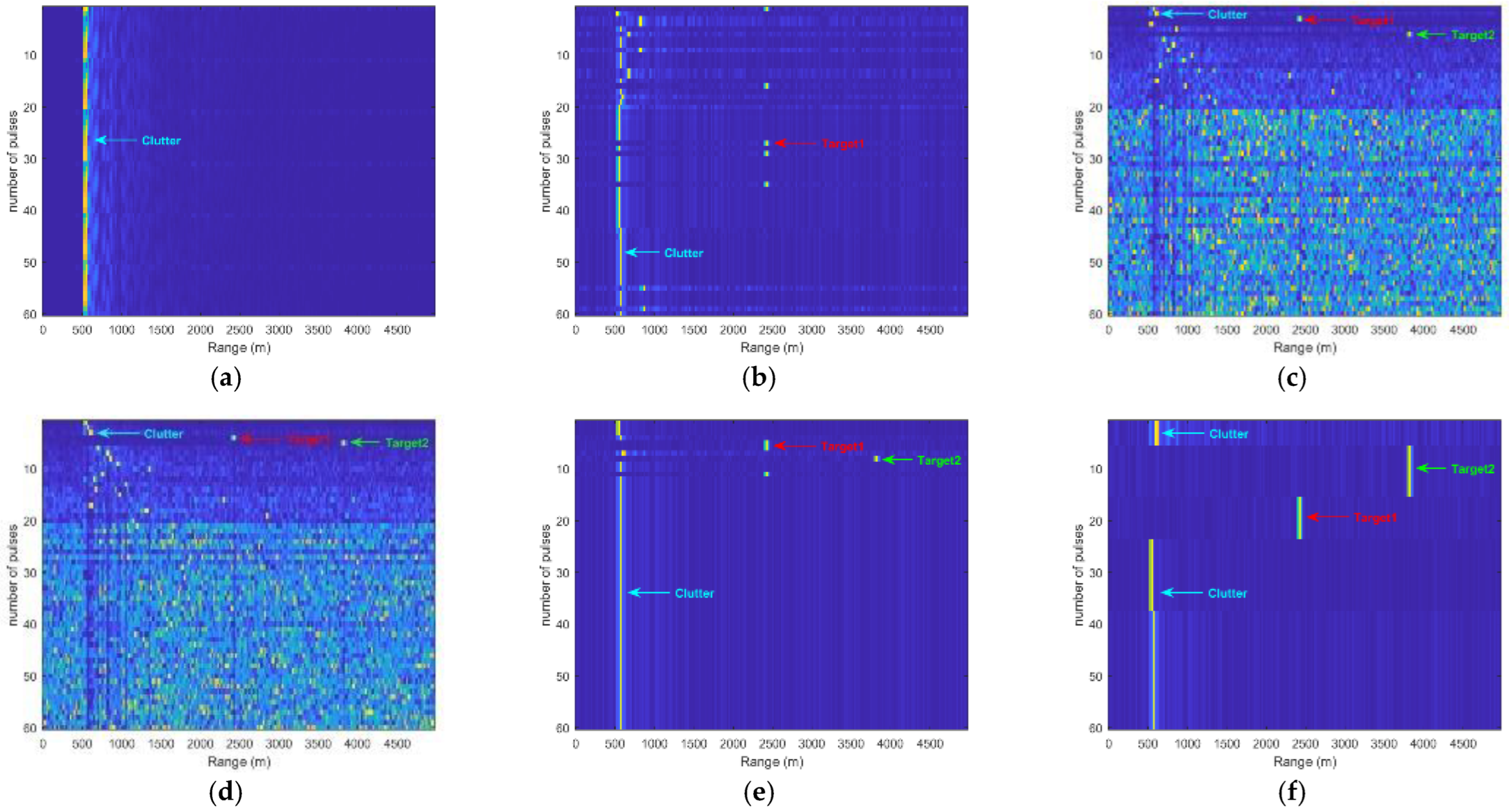
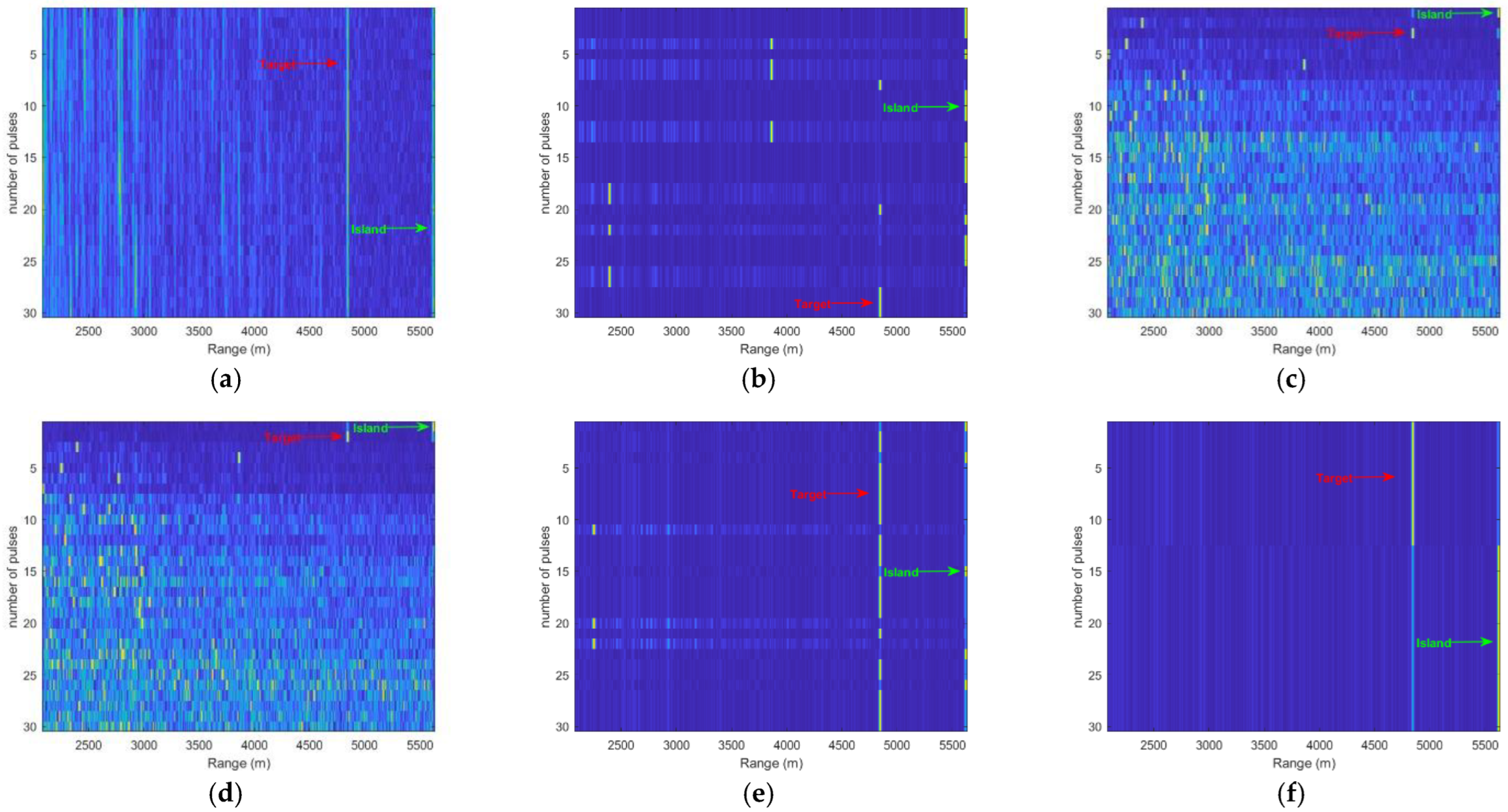
4.4. Experiment 3: Detection of Small Targets in Multi-Channel Complex Background

This section applies the PPSA algorithm to the multi-channel complex background micro-moving target detection problem. In this section, we also use the simulation data set to verify the effect of the PPSA algorithm. We compared the PPSA algorithm with adaptive shifted phase centering (ADPCA) [3], sampling matrix inversion (SMI) [26], FastICA [15], PSA [17], MPSA [18], and NPSA [21]. Quantitative and visual results were compared.

The simulation data set experiment is as follows. In this paper, radar echo data is generated according to the radar system parameters given in

Table 11. Radar system parameters.

Parameter	Numerical Value
pulse repetition frequency/Hz	50000
radar wavelength/m	0.0749
Pulse train length	200
Radar operating frequency range/GHz	4
Antenna height/m	3000
aircraft speed (m/s)	100
Sampling Rate	1 M

and moving targets are generated according to the moving target parameters in

Table 12. Movement target parameters.

Parameter	Sports Goal 1	Sports Goal 2
distance/m	14,457	22,825
radar cross section/m2	1	0.6
radial velocity/m/s	30	60

. It is important to note that the radar transmits and receives signals using a 6-element uniform linear array antenna with antenna elements spaced at half the wavelength of the waveform. The total number of received signals includes return signals from a combination of targets, clutter, noise, and jammers. Finally, we simulated 10 received pulses using the above radar system and moving target parameters. The signal is a data cube of size 200 × 10 × 6. Figure 12a shows the simulated raw signal, where clutter dominates the radar return and masks the target signal. At this stage, we cannot detect the target without further processing. Figure 12b–f show the results of FastICA, PSA, MPSA, NPSA, and PPSA.

As shown in Figure 12a, the clutter is visible, and the clutter completely submerges the target signal. From Figure 12b–d, it can be seen that FastICA, PSA, and MPSA can separate the target. Still, there are many interferences in the results obtained, which is not conducive to subsequent detection processing. From Figure 12e,f, it can be seen that NPSA and PPSA can effectively and accurately separate target 1 and target 2, and the separation effect of PPSA is better. Then, we compare the running time of the above algorithms, and the evaluation time is shown in

Table 13. Running time evaluation of BSS Algorithm.

Method	FastICA	PSA	MPSA	NPSA	PPSA	FastPPSA
Time (s)	5.5095	61.3586	60.9625	74.6430	60.3657	10.7760

.

Table 13 shows that the FastPPSA method still has advantages in running time. The FastICA outperformed the FastPPSA in running time, but its processing effect is poor.

Then we compare the PPSA algorithm with traditional ADPCA and SMI. The results are shown in Figure 13. Figure 13a shows the original signal of the simulation, and Figure 13b–d are the results after noise suppression of the ADPCA, SMI, and PPSA algorithms, respectively.

As shown in Figure 13b, it can be seen that the clutter suppression effect of the ADPCA algorithm is poor, and there are no obvious peaks at target 1 and target 2. Figure 13c shows that after the SMI algorithm processing, a peak appears at target 1, and there is no obvious peak at target 2. Figure 13d shows that the PPSA algorithm can effectively suppress the clutter, and there are obvious peaks where the two targets are located. The quantitative results are shown in

Table 14. SCNR comparison of target 1.

Method	Target 1 Echo Amplitude	Clutter Amplitude Value	SCNR/dB
original signal	0.0103	1.0000	−39.7433
ADPCA	0.4363	0.3821	1.1522
SMI	1.0000	0.0123	38.2019
PPSA	1.0000	0.0135	37.3933

and

Table 15. SCNR comparison of target 2.

Method	Target 2 Echo Amplitude	Clutter Amplitude Value	SCNR/dB
original signal	0.0080	1.0000	−41.9382
ADPCA	0.3148	0.3821	−1.6828
SMI	0.2876	0.0123	6.5317
PPSA	1.0000	0.0165	35.6503

.

Table 14 and Table 15 show that the PPSA method still has advantages in SCR. The PPSA algorithm obtains a slightly lower SNR than that obtained by SMI in target 1, but its SNR in target 2 is much greater than that obtained by SMI. To visually evaluate the clutter effect of the above algorithms, we perform CFAR detection on the results processed by each algorithm. The CFAR detection results are shown in Figure 14.

As shown in Figure 14a, it can be seen that ADPCA cannot effectively detect the target. From Figure 14b, it can be seen that SMI can effectively detect target 1, but cannot detect target 2. Figure 14c,d show that PPSA can effectively detect targets 1 and 2.

Therefore, whether it is the comparison of quantitative results or visual results, the superiority of the PPSA algorithm for clutter suppression of small moving targets in the multi-channel complex background is verified.

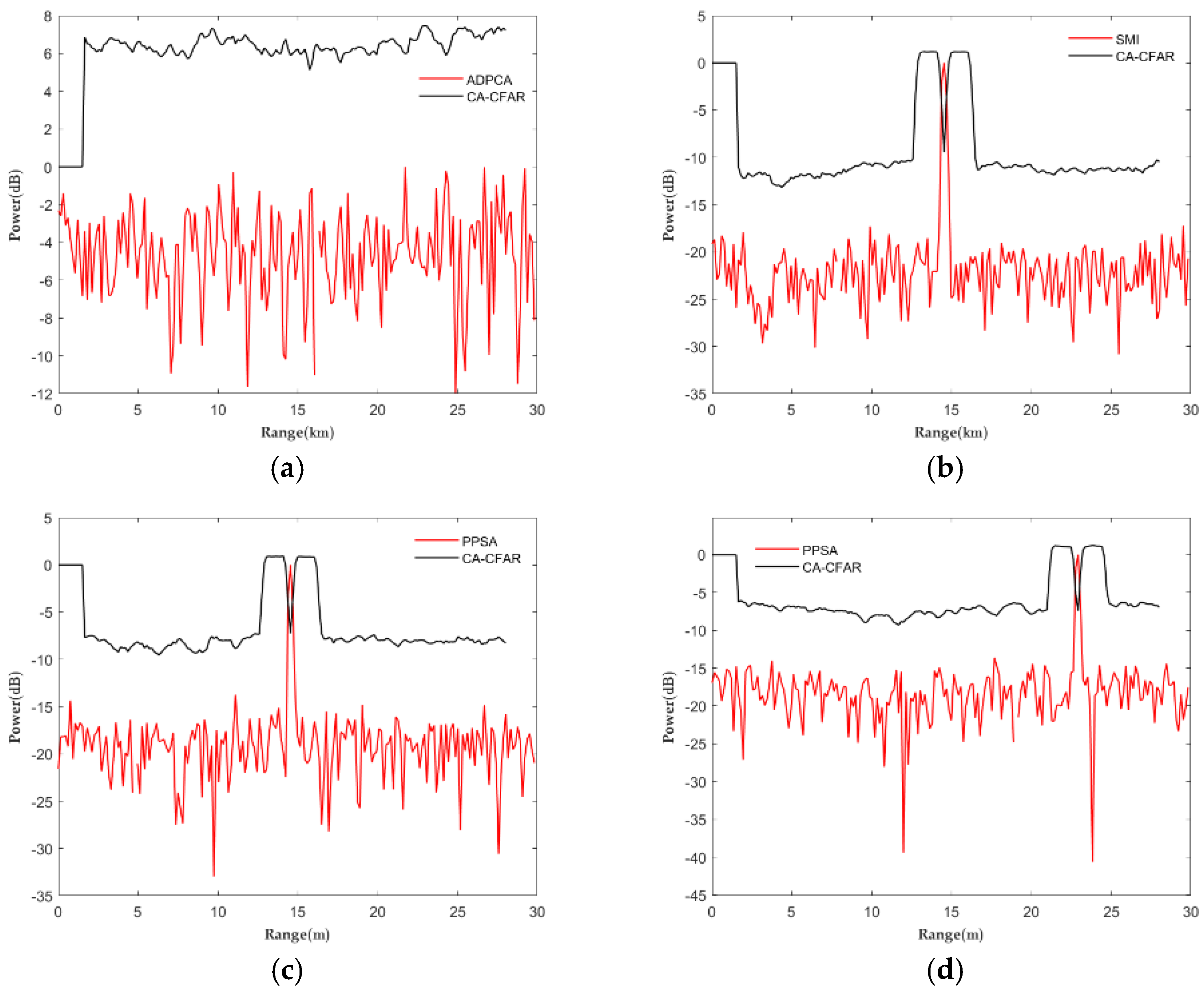
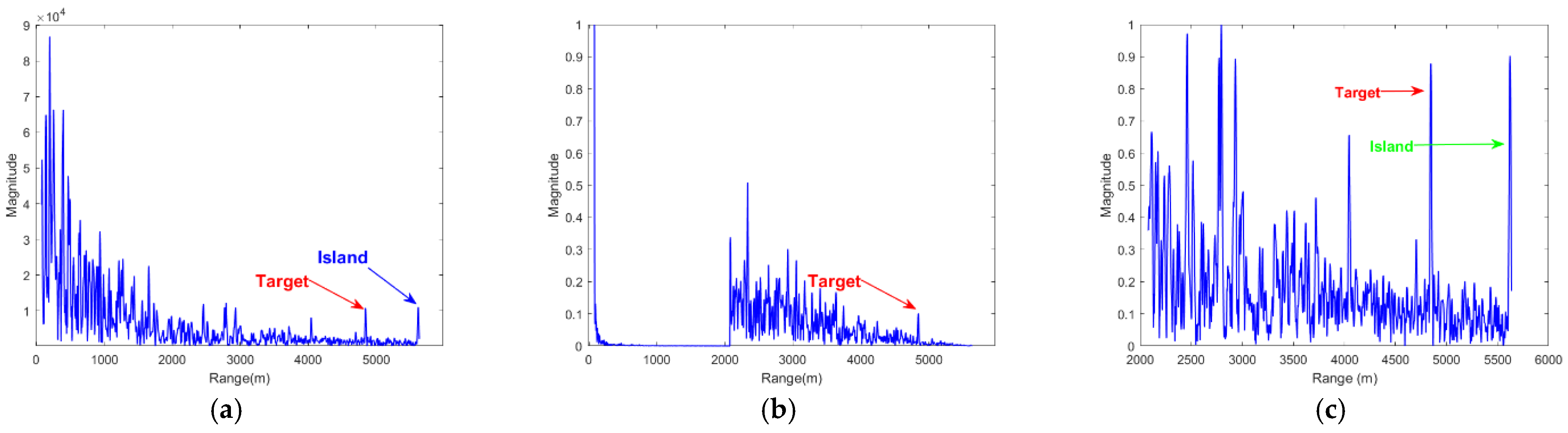
4.5. Experiment 4: Real Radar Echo Data Target Detection Experiment

In this section, we use the measured data to evaluate the performance of the proposed PPSA method. We compared the PPSA algorithm with FastICA [15], PSA [17], MPSA [18], and NPSA [21]. Quantitative and visual results were compared.

The “Radar to Ocean Detection” dataset was measured at the Yangma Island Experimental Site in Yantai in October 2021 [27]. This paper selects the staring mode radar echo data numbered “20210106150614_01_staring.mat” as the test data. The size of the one-dimensional echo signal corresponding to each pulse is 2224, and the number of pulses is 3650. The number of data pulses is enormous; here, we only need to select the first 100 pulses for experimental processing. Due to short-range clutter with solid energy and strong randomness in the radar echo, the false alarm rate of target detection directly on the echo data is very high. Therefore, we first preprocess the echo data. For pulse-echo data with many sampling points, the energy of sea clutter is much larger than that of the target. Therefore, when performing singular value decomposition on such echo data, it is generally believed that the enormous value corresponds to the sea clutter component, and the smaller singular value corresponds to the target and noise components. At the boundary point, the radar echo data can be divided into cluttered and target areas. Only the target area must be detected, significantly reducing the false alarm rate. By SVD processing the above data, we determine the radar echo signal with a distance of less than 2 km as the cluttered area and the rest of the radar echo signal as the target area. We mainly perform object detection on the data of the target area. The target region data is first preprocessed by dimensionality reduction (DR) using the widely used principal component analysis (PCA) method. Here, we select the top 12 main components (PCs) for subsequent analysis because the sum of variances for the top 12 and all PCs is 99.9%. Figure 15a shows the original signal after preprocessing, and Figure 15b–f are the results after noise suppression of algorithms such as FastICA, PSA, MPSA, NPSA, and PPSA, respectively.

As shown in Figure 15a, there is a lot of clutter in the echo, and the target signal is weak. From Figure 15b–d, it can be seen that FastICA, PSA, and MPSA can separate the target, but they have a lot of interference and cannot effectively detect the target. Figure 15e,f shows that NPSA and PPSA can effectively and accurately separate target 1 and target 2, and the separation effect of PPSA is better. Next, we compare the PPSA algorithm with the original echo signal. Figure 16a shows the measured original signal, Figure 16b is the result after SVD processing, Figure 16c is the target area, and Figure 16d is the result after noise sup-pression by the PPSA algorithm.

As shown in Figure 16, it can be seen that the PPSA algorithm can effectively suppress clutter. The quantitative results are shown in

Table 16. SCNR comparison of target 1.

Method	Target 1 Echo Amplitude	Clutter Amplitude Value	SCNR/dB
original signal	0.8767	0.1798	13.7612
noncoherent	0.9425	0.1384	16.6639
coherent	1.0000	0.0342	29.3310
PPSA	1.0000	0.0242	32.3237

.

Table 16 shows that the SCR of the target is significantly improved after processing by the PPSA algorithm. To evaluate the clutter effect of the above algorithms, we performed CFAR detection on the results processed by the PPSA algorithm. This section adopts the unit average CFAR. The false alarm probability is (10-6), the protection unit is 5, and the reference unit is 15. The target detection results are shown in Figure 17.

As shown in Figure 17, it can be seen that CFAR detection directly on the target area cannot effectively detect the target. However, after the clutter suppression by the PPSA algorithm, the target can be effectively detected.

Therefore, comparing quantitative and visual results both verify the effectiveness of the PPSA algorithm in suppressing clutter.

In addition, we also compare the running speed of the above FastICA, PSA, MPSA, NPSA, PPSA and FastPPSA algorithms. Figure 18 plots thesix algorithms’ running time curves at different frequency bands.

As shown in Figure 18, it can be seen that the time consumption of FastPPSA is less than other algorithms. Each iteration of FastICA needs to involve all pixels to find the best projection direction, which means that the more pulse-echo sampling points, the more time it takes to solve. FastPPSA uses Parfor parallel computing, which makes it faster when dealing with high-dimensional data.

5. Conclusions

Aiming at the problem that the existing PSA algorithm cannot accurately obtain the real solution, this paper improves the original PSA algorithm and proposes a high-precision parallel PSA algorithm. Unlike the current PSA algorithm that solves eigenpairs serially, the PPSA algorithm no longer imposes any constraints. Still, it selects the eigenvectors of the forward tensor slice as the initial value for a free iterative solution, effectively avoiding the imposition of constraints error. By comparing the algorithm with the existing PSA algorithm, it is verified that it has better accuracy and robustness in blind image separation and radar target detection.

It should be noted that PSA, NPSA, and PPSA all focus on the third-order skewness of the dataset. For other datasets, skewness may not always be the best choice. In this case, other metrics, such as fourth-order kurtosis or higher-order statistics, can be used instead.

References

1. Bakr, O.; Johnson, M.; Mudumbai, R.; Ramchandran, K. Multi-antenna interference cancellation techniques for cognitive radio applications. In Proceedings of the 2009 IEEE Wireless Communications and Networking Conference, Budapest, Hungary, 5–8 April 2009; pp. 1–6. [Google Scholar]
2. Muehe, C.E.; Labitt, M. Displaced-phase-center antenna technique. Linc. Lab. J. 2000, 12, 281–296. [Google Scholar]
3. Pour, Z.A.; Shafai, L. Adaptive aperture antennas with adjustable phase centre locations. In Proceedings of the 2012 IEEE International Workshop on Antenna Technology (iWAT), Tucson, AZ, USA, 5–7 March 2012; pp. 355–357. [Google Scholar]
4. Brennan, L.E.; Reed, L. Theory of adaptive radar. IEEE Trans. Aerosp. Electron. Syst. 1973, AES-9, 237–252. [Google Scholar] [CrossRef]
5. Wang, Z.; Chen, W.; Zhang, T.; Xing, M.; Wang, Y. Improved Dimension-Reduced Structures of 3D-STAP on Nonstationary Clutter Suppression for Space-Based Early Warning Radar. Remote Sens. 2022, 14, 4011. [Google Scholar] [CrossRef]
6. Knudsen, K.S.; Bruton, L.T. Mixed domain filtering of multidimensional signals. IEEE Trans. Circuits Syst. Video Technol. 1991, 1, 260–268. [Google Scholar] [CrossRef]
7. Klemm, R. Antenna design for adaptive airborne MTI. In Proceedings of the 92 International Conference on Radar, Brighton, UK, 12–13 October 1992; pp. 296–299. [Google Scholar]
8. Gui, R.; Wang, W.Q.; Farina, A.; So, H.C. FDA radar with doppler-spreading consideration: Mainlobe clutter suppression for blind-doppler target detection. Signal Process. 2021, 179, 107773. [Google Scholar] [CrossRef]
9. Weinberg, G.V. Constant false alarm rate detectors for Pareto clutter models. IET Radar Sonar Navig. 2013, 7, 153–163. [Google Scholar] [CrossRef]
10. Jia, F.; Sun, G.; He, Z.; Li, J. Grating-lobe clutter suppression in uniform subarray for airborne radar STAP. IEEE Sens. J. 2019, 19, 6956–6965. [Google Scholar] [CrossRef]
11. Qian, L. Radar clutter suppression solution based on ICA. In Proceedings of the 2013 Fourth International Conference on 189Intelligent Systems Design and Engineering Applications, Zhangjiajie, China, 6–7 November 2013; pp. 429–432. [Google Scholar]
12. Karlsen, B.; Larsen, J.; Sorensen, H.B.; Jakobsen, K.B. Comparison of PCA and ICA based clutter reduction in GPR systems for anti-personal landmine detection. In Proceedings of the Proceedings of the 11th IEEE Signal Processing Workshop on Statistical Signal Processing (Cat. No. 01TH8563), Singapore, 8 August 2001; pp. 146–149. [Google Scholar]
13. Tannous, O.; Kasilingam, D. Independent component analysis of polarimetric SAR data for separating ground and vegetation components. In Proceedings of the 2009 IEEE International Geoscience and Remote Sensing Symposium, Cape Town, South Africa, 12–17 July 2009; Volume 4, pp. IV-93–IV-96. [Google Scholar]
14. Comon, P. Independent component analysis, a new concept? Signal Process. 1994, 36, 287–314. [Google Scholar] [CrossRef]
15. Hyvarinen, A. Fast and robust fixed-point algorithms for independent component analysis. IEEE Trans. Neural Netw. 1999, 10, 626–634. [Google Scholar] [CrossRef] [PubMed] [Green Version]
16. Oja, E.; Yuan, Z. The FastICA algorithm revisited: Convergence analysis. IEEE Trans. Neural Netw. 2006, 17, 1370–1381. [Google Scholar] [CrossRef] [PubMed] [Green Version]
17. Geng, X.; Ji, L.; Sun, K. Principal skewness analysis: Algorithm and its application for multispectral/hyperspectral images indexing. IEEE Geosci. Remote Sens. Lett. 2014, 11, 1821–1825. [Google Scholar] [CrossRef]
18. Geng, X.; Meng, L.; Li, L.; Ji, L.; Sun, K. Momentum principal skewness analysis. IEEE Geosci. Remote Sens. Lett. 2015, 12, 2262–2266. [Google Scholar] [CrossRef] [Green Version]
19. Meng, L.; Geng, X.; Ji, L. Principal kurtosis analysis and its application for remote-sensing imagery. Int. J. Remote Sens. 2016, 37, 2280–2293. [Google Scholar] [CrossRef]
20. Anandkumar, A.; Ge, R.; Hsu, D.; Kakade, S.M.; Telgarsky, M. Tensor decompositions for learning latent variable models. J. Mach. Learn. Res. 2014, 15, 2773–2832. [Google Scholar]
21. Geng, X.; Wang, L. NPSA: Nonorthogonal principal skewness analysis. IEEE Trans. Image Process. 2020, 29, 6396–6408. [Google Scholar] [CrossRef] [PubMed] [Green Version]
22. Kolda, T.G.; Bader, B.W. Tensor decompositions and applications. SIAM Rev. 2009, 51, 455–500. [Google Scholar] [CrossRef]
23. Lim, L.H. Singular values and eigenvalues of tensors: A variational approach. In Proceedings of the 1st IEEE International Workshop on Computational Advances in Multi-Sensor Adaptive Processing, Puerto Vallarta, Mexico, 13–15 December 2005; p. 129. [Google Scholar]
24. Qi, L. Eigenvalues of a real supersymmetric tensor. J. Symb. Comput. 2005, 40, 1302–1324. [Google Scholar] [CrossRef] [Green Version]
25. Wang, L.; Geng, X. The real eigenpairs of symmetric tensors and its application to independent component analysis. IEEE Trans. Cybern. 2021, 52, 10137–10150. [Google Scholar] [CrossRef] [PubMed]
26. Guerci, J.R. Space-Time Adaptive Processing for Radar; Artech House: Norwood, MA, USA, 2014. [Google Scholar]
27. Ningbo, L.; Hao, D.; Yong, H.; Yunlong, D.; Guoqing, W.; Kai, D. Annual progress of the sea-detecting X-band radar and data acquisition program. J. Radars 2021, 10, 173–182. [Google Scholar]
Figure 1. Slices of a third-order tensor. (a) horizontal slices, (b) lateral slices, (c) lateral slices.
Remotesensing 15 00288 g001
Figure 2. The distribution of two true eigenvectors, and those obtained by PSA and MPSA in a unit circle. (a) The first result was obtained with PSA and MPSA; (b) the second result was obtained by PSA and MPSA.
Remotesensing 15 00288 g002
Figure 3. The distribution of two true eigenvectors, and those obtained by NPSA in a unit circle. (a) The first result was obtained with NPSA; (b) the second result was obtained by NPSA.
Remotesensing 15 00288 g003
Figure 4. The distribution of two true eigenvectors, and those obtained by PPSA in a unit circle.
Remotesensing 15 00288 g004
Figure 5. The results of FastICA, PSA, MPSA, NPSA, MSDP and PPSA. The first and second column are the three source images and randomly mixed images as the reference. (a) source image 1, (b) source image 2, (c) source image 3, (d) mixed image 1, (e) mixed image 2, (f) mixed image 3, (g) IC1 of FastICA, (h) IC2 of FastICA, (i) IC3 of FastICA, (j) IC1 of PSA, (k) IC2 of PSA, (l) IC3 of PSA, (m) IC1 of MPSA, (n) IC2 of MPSA, (o) IC3 of MPSA, (p) IC1 of NPSA, (q) IC2 of NPSA, (r) IC3 of NPSA, (s) IC1 of MSDP, (t) IC2 of MSDP, (u) IC3 of MSDP, (v) IC1 of PPSA, (w) IC2 of PPSA, (x) IC3 of PPSA.
Remotesensing 15 00288 g005
Figure 6. The results of FastICA, PSA, MPSA, NPSA and PPSA. (a) echo data, (b) the result of FastICA, (c) the result of PSA, (d) the result of MPSA, (e) the result of NPSA, (f) the result of PPSA.
Remotesensing 15 00288 g006
Figure 7. The results of incoherent accumulation, coherent accumulation and PPSA. (a) Echo data, (b) the result of incoherent accumulation, (c) the result of coherent accumulation, (d) the result of PPSA.
Remotesensing 15 00288 g007
Figure 8. The CFAR detection results for incoherent accumulation, coherent accumulation and PPSA. (a) The results of incoherent accumulation, (b) the results of coherent accumulation, (c) the results of PPSA 1, (d) the results of PPSA 2.
Remotesensing 15 00288 g008
Figure 9. The BSS results for FastICA, PSA, MPSA, NPSA, and PPSA. (a) Echo data, (b) the result of FastICA, (c) the result of PSA, (d) the result of MPSA, (e) the result of NPSA, (f) the result of PPSA.
Remotesensing 15 00288 g009
Figure 10. The clutter suppression results for TPC, SPC, and PPSA. (a) Echo data, (b) the result of TPC, (c) the result of SPC, (d) the result of PPSA.
Remotesensing 15 00288 g010
Figure 11. The CFAR detection results for TPC, SPC, and PPSA. (a) The result of TPC, (b) the result of SPC, (c) the result of PPSA, (d) the result of PPSA.
Remotesensing 15 00288 g011
Figure 12. The BSS results for FastICA, PSA, MPSA, NPSA, and PPSA. (a) Echo data, (b) the result of FastICA, (c) the result of PSA, (d) the result of MPSA, (e) the result of NPSA, (f) the result of PPSA.
Remotesensing 15 00288 g012
Figure 13. The clutter suppression results for ADPCA, SMI, and PPSA. (a) Echo data, (b) the result of ADPCA, (c) the result of SMI, (d) the result of PPSA.
Remotesensing 15 00288 g013
Figure 14. The CFAR detection results for ADPCA, SMI, and PPSA. (a) The result of ADPCA, (b) the result of SMI, (c) the result of PPSA, (d) the result of PPSA.
Remotesensing 15 00288 g014
Figure 15. The BSS results for FastICA, PSA, MPSA, NPSA, and PPSA. (a) Echo data, (b) the result of FastICA, (c) the result of PSA, (d) the result of MPSA, (e) the result of NPSA, (f) the result of PPSA.
Remotesensing 15 00288 g015
Figure 16. The clutter suppression results for PPSA. (a) Echo data, (b) the result of SVD, (c) the result of the target area, (d) the result of noncoherent accumulation, (e) the result of coherent accumulation, (f) the result of PPSA.
Remotesensing 15 00288 g016aRemotesensing 15 00288 g016b
Figure 17. The CFAR detection results for PPSA. (a) The result of target area, (b) the result of noncoherent accumulation, (c) the result of coherent accumulation, (d) the result of PPSA.
Remotesensing 15 00288 g017aRemotesensing 15 00288 g017b
Figure 18. Time consumption comparison of FastICA, PSA, MPSA, NPSA, PPSA, and FastPPSA.
Remotesensing 15 00288 g018