Article

Towards Unified Online-Coupled Aerosol Parameterization for the Brazilian Global Atmospheric Model (BAM): Aerosol–Cloud Microphysical–Radiation Interactions

by
Jayant Pendharkar
1,
Silvio Nilo Figueroa
1,
Angel Vara-Vela
2,3,4,
R. Phani Murali Krishna
5,
Daniel Schuch
6,
Paulo Yoshio Kubota
1,
Débora Souza Alvim
1,7,
Eder Paulo Vendrasco
1,
Helber Barros Gomes
8,
Paulo Nobre
1 and
Dirceu Luís Herdies
1,*
1
National Institute for Space Research (INPE), Cachoeira Paulista, São José dos Campos 12227-010, SP, Brazil
2
Department of Geoscience, Aarhus University, 8000 Aarhus, Denmark
3
Department of Physics and Astronomy, Aarhus University, 8000 Aarhus, Denmark
4
iCLIMATE Aarhus University Interdisciplinary Centre for Climate Change, Aarhus University, 4000 Roskilde, Denmark
5
Indian Institute of Tropical Meteorology, Pune 411008, India
6
Department of Civil and Environmental Engineering, Northeastern University, Boston, MA 02115, USA
7
Lorena School of Engineering (EEL), University of Sao Paulo (USP), Lorena 12602-810, SP, Brazil
8
Institute of Atmospheric Sciences, Federal University of Alagoas, Maceio 57072-900, AL, Brazil
*
Author to whom correspondence should be addressed.
Remote Sens. 2023, 15(1), 278; https://doi.org/10.3390/rs15010278
Submission received: 20 November 2022 / Revised: 27 December 2022 / Accepted: 29 December 2022 / Published: 3 January 2023
(This article belongs to the Section Atmospheric Remote Sensing)

Abstract

:
In this work, we report the ongoing implementation of online-coupled aerosol–cloud microphysical–radiation interactions in the Brazilian global atmospheric model (BAM) and evaluate the initial results, using remote-sensing data for JFM 2014 and JAS 2019. Rather than developing a new aerosol model, which incurs significant overheads in terms of fundamental research and workforce, a simplified aerosol module from a preexisting global aerosol–chemistry–climate model is adopted. The aerosol module is based on a modal representation and comprises a suite of aerosol microphysical processes. Mass and number mixing ratios, along with dry and wet radii, are predicted for black carbon, particulate organic matter, secondary organic aerosols, sulfate, dust, and sea salt aerosols. The module is extended further to include physically based parameterization for aerosol activation, vertical mixing, ice nucleation, and radiative optical properties computations. The simulated spatial patterns of surface mass and number concentrations are similar to those of other studies. The global means of simulated shortwave and longwave cloud radiative forcing are comparable with observations with normalized mean biases ≤11% and ≤30%, respectively. Large positive bias in BAM control simulation is enhanced with the inclusion of aerosols, resulting in strong overprediction of cloud optical properties. Simulated aerosol optical depths over biomass burning regions are moderately comparable. A case study simulating an intense biomass burning episode in the Amazon is able to reproduce the transport of smoke plumes towards the southeast, thus showing a potential for improved forecasts subject to using near-real-time remote-sensing fire products and a fire emission model. Here, we rely completely on remote-sensing data for the present evaluation and restrain from comparing our results with previous results until a complete representation of the aerosol lifecycle is implemented. A further step is to incorporate dry deposition, in-cloud and below-cloud scavenging, sedimentation, the sulfur cycle, and the treatment of fires.

1. Introduction

Aerosols play an important role in regulating Earth’s radiation budget by scattering and absorbing incident solar radiation and its reflected component from the surface (direct effect) [1]. Their role in the indirect effect is more complex and entails modifying cloud microphysical and radiative properties. Aerosols serve as cloud condensation nuclei (CCN) and ice nuclei (IN), resulting in an increase in cloud droplet number concentration (CDNC), ice particle concentration, and cloud albedo [2,3,4]. Not long after the discovery, several centers across the globe began modeling their effects in general circulation models (GCMs); however, there remains an uncertainty in quantifying their impacts on the present day and future climate [5,6,7]. Globally, the contribution to these effects made by anthropogenic aerosols is estimated to impart a net cooling at the top of the atmosphere [5]. Uncertainty in the estimation can be attributed to several factors, which include principally the preferred mode of coupling (online or offline) aerosol–climate interactions, followed by the accurate modeling of the aerosol size distributions; their influence on cloud processes; the correct representation of physical properties; and the mixing states, whether external (distinct) or internal (mixed with other aerosol particles). In a unified online-coupled model, an aerosol module is integrated into the GCM, allowing the aerosol processes and feedbacks to be treated consistently with meteorological processes in the same time step. This mode of coupling has shown a better performance in regard to representing the spatiotemporal variability of aerosol distribution and radiative forcing, relative to its offline counterpart [8]. However, an improvement in performance is determined by the details of the complexity represented in the model and comes at the expense of heavy computational time. To help place the aforementioned factors into context, Supplementary Table S1 lists a few studies that briefly summarize the uncertainties in the estimation of radiative forcings for carbonaceous aerosols—black carbon (BC), sulfate, secondary organic aerosol (SOA), dust (DU), and sea salt (SS). For instance, given the warming effect caused by BC, the simulated radiative forcing from offline models is observed to be negative contrary to the online-coupled models [9,10,11,12]. In the case of sulfate, models using a physically based approach yield improved results over models using an empirically based relation [13,14,15,16,17]. The uncertainties can be constrained depending on the correct representation of SOA formation pathways [18,19,20,21]. The complexity in representing the DU cycle in global models results in a variation in simulated emissions by a factor of two [22,23,24,25,26,27,28,29,30,31,32,33]. Lastly, correct representation of the size distribution, loading, and production mechanism of SS in global models can constrain the indirect effect [34,35,36,37,38].
The South American continent exhibits a rich diversity in sources and sinks, characteristics, and spatiotemporal variability of natural and anthropogenic aerosols, viz a giant Amazon ecosystem; biomass burning occurring in the dry season related to cultivation, deforestation, and annual forest fires; pollution from industrial and economic zones; and advection via mesoscale systems [39,40,41,42,43,44,45,46,47]. This diversity adds to the existing challenges in representing aerosols and their parameterizations in GCMs. The Atmospheric Chemistry and Climate Model Intercomparison Project (ACCMIP) involved the participation of about 16 models simulating several time slices (1850–2100) of experiments to obtain an insight into the role of atmospheric chemistry on historical, present, and future climate [48]. About 50% are coupled chemistry–climate models. Shindell et al. [49] evaluated the simulated radiative forcings and aerosol optical depths (AODs) against observations for South America (SA). The annual averaged multi-model mean 550 nm AOD over areas of intense biomass burning is underpredicted (0.15–0.25) compared to satellite observations (0.25–0.45). The spatial extent of the AOD in these areas is underestimated, as well. For the absorbing BC aerosols that can cause positive forcing, the model-simulated absorbing AOD is poorly correlated with satellite data and underestimated by about a factor of two, and the multi-model mean shows negative biases. The inability to capture the transport of aerosols and the missing SOA and nitrate in many models is indicated as a possible reason for the underestimation. A related study using eight coupled chemistry–climate simulations from ACCMIP reports that, despite using the same anthropogenic and biomass burning emissions, models differ significantly in simulating the present-day black carbon burden and deposition fluxes over the southern hemisphere owing to different aerosol-removal mechanisms and the atmospheric state [50].
In another study by Alvim et al. [51], simulated AOD from two global online-coupled aerosol–chemistry–climate models, namely the European Centre Hamburg Model–Hamburg Aerosol Model (ECHAM–HAM) and the Community Atmosphere Model–Modal Aerosol Model (CAM5–MAM3), for the period 2001–2006, are compared with ground-based and satellite observations. Both the models run at about 2° × 2° resolution, with about 30 vertical levels, and use AeroCom II emission fluxes. The simulated seasonal mean 550 nm AOD over South America shows an overall negative bias for all seasons in both models. During the biomass burning season, the underestimation is largest. Next, the simulated monthly mean AOD averaged over 2001–2006 for sites lying around the arc of deforestation, namely Alta Floresta, Rio Branco, and Cuiaba, is compared with the observed AOD and number of fire occurrences. Both models show inconsistencies in representing the AOD variability in the dry season. Extending along the same lines, Alvim et al. [45] used the chemistry component of CAM to study the influence of biomass burning on air pollution by comparing it with the observed carbon monoxide (CO) and Fire Radiative Power (FRP). Two experiments were performed at similar resolutions as the previous study, but for the period 2009–2014—one with tropospheric chemistry and the other with tropospheric and stratospheric chemistry. The study has shown that the inclusion of detailed chemistry, along with removal mechanism, reduces the positive bias in the simulated CO but overestimates AOD, with a high correlation between FRP, CO, and AOD over the arc of deforestation and at the transition between forest and savanna during the biomass burning season in both experiments. The authors conclude that the inclusion of complexity shows improvement in some regions but adversely affects other parameters.
From the studies referred to above, the following can be inferred: (a) Accurate representation of aerosols and their lifecycle in a numerical model is a challenging task because of their complex mechanisms and their influence on meteorology and vice versa; in other words, the feedbacks are still not completely understood. (b) Online-coupled global aerosol–climate models are more veritable in simulating climate. (c) Most of the existing global models show biases in simulating aerosols over SA. Thus, it becomes imperative to implement aerosol interactions coupled online to the Brazilian global atmospheric model (BAM) [52], which currently is the operational numerical weather and subseasonal-to-seasonal (S2S) prediction model at the Centre for Weather Forecast and Climate Studies (CPTEC) and also forms the atmospheric component of the Brazilian Earth System Model (BESM) [53,54,55] used for climate-prediction and climate-change studies. This paper describes the CPTEC’s initiative to incorporate aerosol interactions into its global model, as well as preliminary results. Over the last three decades, BAM has continuously developed to improve weather/climate prediction and atmospheric dynamics studies. BAM can be run in several configurations depending on the objective of the study and available computational resources, for example, using simplified and fast physics (single-moment cloud microphysics, radiation absorption, and scattering over eleven spectral bands, a simplified biosphere model) for climate integrations that include an Eulerian advection scheme; detailed physics (double-moment cloud microphysics, a dynamic vegetation model, and a complex radiation transfer model) with a semi-Lagrangian advection scheme for operational purposes; and other combinations [52,56]. Climate studies using BAM have demonstrated its ability to well represent the determinants of climate variability and teleconnection patterns. However, there are a few areas that require improvements: weak cloud radiative forcing at TOA, overestimation of precipitation in Southeast SA, latent heating, and sensible heat fluxes [57,58,59]. Performance evaluation in operational mode showed improved tropical precipitation with modified convective parameterization and S2S prediction being comparable to similar models from leading centers [60].
Given the numerous years of extensive research and human resources invested by leading centers in developing state-of-the-science global aerosol–chemistry–climate models, the approach to implementing online-coupled aerosol interactions in BAM is to adopt a simplified aerosol representation instead of developing a new (better) aerosol model, and then later extend it to include more complex aerosol processes. The aerosol representation chosen for BAM is a simplified aerosol microphysics (hereafter, referred to as AMIC) module developed at the Pacific Northwest National Laboratory (PNNL) to test aerosol microphysics processes offline. The module was extended and implemented in the Model for Integrated Research on Atmospheric Global Exchanges (MIRAGE) [61] and the National Center for Atmospheric Research’s CAM–MAM [62,63]. Thus, the AMIC module made available to the CPTEC can be considered as a subset (described below in Section 2.1) of CAM–MAM. In this work, we present the implementation of AMIC in BAM. In order to evaluate its performance, feedback is given to the cloud microphysics and radiation schemes in BAM. It is important to note here that AMIC in BAM also provides a structural framework for the inclusion of aerosols and that the task of implementing the feedback is substantial, given the fact that the dynamics and physical parameterizations of the GCMs in online-coupled models (e.g., CAM or ECHAM) have undergone significant enhancements to incorporate aerosol parameterization. The implementation of AMIC feedback enables us to simulate the direct and indirect effects of aerosols, that is, the formation of CCN, changes in CDNC, computation of radiative optical properties, and the resulting radiative forcings. We also note that, for the partial representation of aerosol processes implemented in BAM until now, we rely heavily on remote-sensing observations for evaluation. Comparing the results with previous results from existing global aerosol models requires a complete representation of the aerosol processes in BAM, and this is not viable or conclusive at the current stage of implementation. Therefore, the BAM global simulations are compared with satellite observations, which provide global data. Section 2 describes the implementation of AMIC and its feedback in BAM. Section 3 describes the experimental design and observational datasets used for the model evaluation. The model evaluation, using remote sensing data, is presented in Section 4. Section 5 concludes the presented work with future directions.

2. Model Development

The version of BAM used in this work is the operational version with sigma vertical coordinates. Cloud microphysics by Morrison double-moment scheme [64] predicts mass and number mixing ratios of five hydrometeors, viz cloud droplets, ice, rain, snow, and graupel. The SW and LW radiation scheme is the Rapid Radiative Transfer Model for GCMs (RRTMG) by Iacono et al. [65]. Shallow convection is the Tiedtke [66] diffusion scheme. Deep convection is the Arakawa and Schubert [67] scheme. The land-surface scheme is the Integrated Biosphere Simulator (IBIS) [68,69,70]. In this section, we first describe the AMIC module, followed by the modifications performed in BAM to account for the feedbacks, and finally the aerosol inputs in BAM.

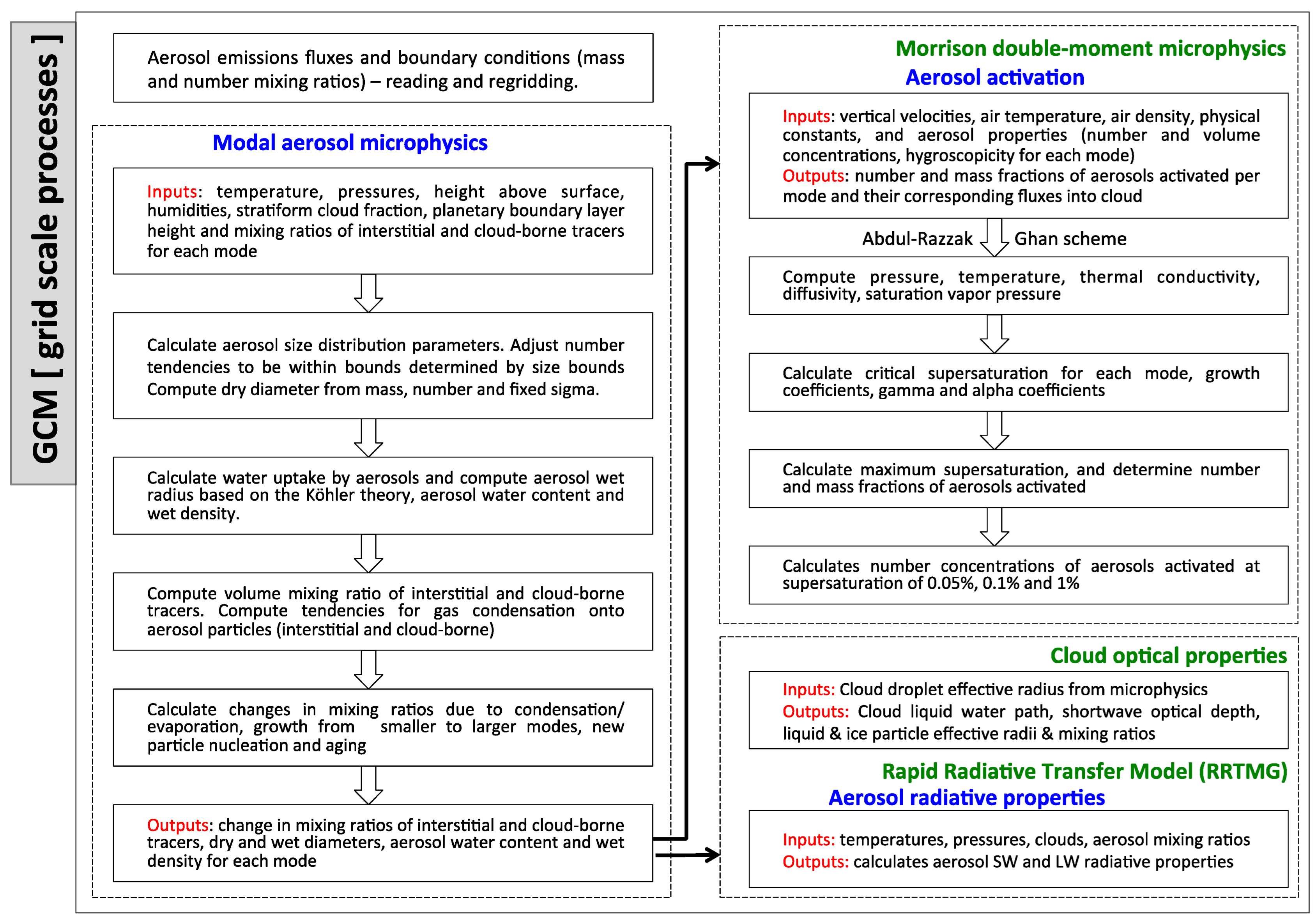
2.1. AMIC—The Aerosol Module for BAM

The aerosol species include sulfate, ammonium, nitrate, primary organic matter (POM), SOA, BC, SS, and DU. The modal approach is adopted where particle size distribution is approximated by lognormal distributions representing modes of particle population. Each mode has multiple species. Within each mode, internal mixing is assumed. Two types of aerosols are treated: interstitial (particles suspended in clear air) and cloud borne (particles attached to cloud droplets). Six trace gases are transported: sulfur dioxide (SO2), hydrogen peroxide (H2O2), dimethyl sulfide (DMS), sulfuric acid gas vapor (H2SO4), ammonia (NH3), and a lumped semi-volatile organic species (SOAG). The aerosol module, like in CAM–MAM, can be run in three modes: a detailed 7-mode (MAM7) with Aitken, accumulation, primary carbon, and fine and coarse modes for dust and sea salt with 31 tracers; a simplified 3-mode (MAM3) with Aitken, accumulation, and coarse modes with 15 tracers suitable for long-term simulations; and a 4-mode (MAM4) with inclusion of a primary carbon mode for treating carbonaceous materials [62,63]. AMIC comprises a suite of aerosol microphysics processes, namely, gas–aerosol exchange, renaming, nucleation, coagulation, and aging. The size representation is achieved by using one or more lognormally distributed modes characterized by number concentration, geometric mean diameter (DgN), and geometric standard deviation (σg). For each mode, both mass (qi) and number (Ni) mixing ratios are predicted by assuming a fixed σg (used in other global climate–aerosol models, viz [61,71]). Moreover, qi and Ni determine the dry sizes, DgN. Gas phase chemistry computes only the loss of SO2 to H2SO4, taking into account the SO2 lifetime of ~2 days. Aqueous-phase chemistry includes the absorption of SO2, H2SO4, and NH3 in cloud water and the production of aqueous-phase sulfate. The production of sulfate from SO2 and H2SO4 occurs in all modes, and its partitioning among each mode is proportionate to the number mixing ratio of cloud-borne species in each mode. The timescale of SO2 absorption is 30 min. Water uptake by aerosols is based on the Köhler theory. For each mode, the aerosol wet radius is calculated from the dry radius, using ambient relative humidity and volume mean hygroscopicity [72]. The aerosol water content and wet density for each mode are computed by using single-particle mean dry and wet volume and water volume. For the clear subarea of a grid cell, gas–aerosol exchange treats simultaneous condensation and evaporation of H2SO4 and SOA gas onto particles, using the Fuchs–Sutugin growth relation, with an accommodation coefficient of 0.65 for H2SO4 [73,74,75]. Homogeneous nucleation of H2SO4 and water vapor resulting in the formation of new particles and their subsequent growth to Aitken mode follows Vehemaki et al. [76] and Kerminen and Kulmala’s [77] parameterization. Renaming involves transferring the larger Aitken-mode particles, which grow as a result of gas condensation and aqueous sulfate production, to the accumulation mode, following Wilson [78]. Coagulation (coalescence) of particles reduces the number concentration, conserving the mass and shifting the size distribution towards larger sizes (Aitken to accumulation mode and Aitken to primary carbon to accumulation mode), following Binkowski and Roselle [79]. Condensation onto the carbonaceous particles and coagulation result in the conversion from hydrophobic to hydrophilic (accumulation) mode (referred to as aging process), involving sulfate and SOA. For the cloudy subarea of a grid cell, renaming, gas–aerosol exchange, and aging of particles are computed if condensation is applicable, but only renaming of particles is calculated otherwise. New particle nucleation and coagulation are not performed in the cloudy subarea. Figure 1 summarizes the AMIC module and incorporation of feedback.

2.2. Feedbacks between AMIC and BAM

2.2.1. Aerosol–Cloud Interactions

To simulate the aerosol–cloud interactions, aerosol activation and ice nucleation were implemented in the Morrison double-moment cloud microphysics scheme. Activation refers to the cloud process where interstitial aerosols are converted to cloud-borne aerosols, and this determines the number of cloud droplets nucleated. The number and mass fraction activated or, equivalently, the cloud droplets nucleated, are based on the Köhler theory, where the number activated is expressed in terms of supersaturation [80]. In global models with multiple aerosols, calculating supersaturation is computationally expensive, so physically based parameterization is used instead. Currently, the Morrison scheme provides two options: a constant CDNC of 250 cm−3 with CCN spectra following a power-law; and using a two-mode lognormal size distribution to derive CCN spectra with fixed DgN (=0.052 μm, 1.3 μm), σg (=2.04, 2.5), and number concentration (=72.2 × 10⁶ m−3, 1.8 × 10⁶ m−3), respectively, for Modes 1 and 2. With AMIC implemented, the two options are replaced with aerosol activation parameterization by Abdul-Razzak and Ghan (hereafter, AG00) [81]. AG00 simulates the activation of cloud droplets due to multiple aerosols. The droplets formed are parameterized in terms of updraft velocity, temperature, density of the air parcel, aerosol number concentration and size distribution, DgN, and volume mean hygroscopicity of each aerosol mode. Strong updrafts or low aerosol number concentrations result in higher supersaturations activating most of the aerosols. However, for weak updrafts, supersaturations affect the number activated less, and CDNC may not be equal to the number of droplets nucleated. Ghan et al. [82] predicted CDNC by accounting for the number nucleated, turbulent transport and droplet loss due to dissipation of clouds. Aerosol activation consistent with the prognostic treatment of droplet nucleation is implemented in BAM. The parameterization of ice nucleation is based on Liu and Penner [83] and replaces the Cooper [84] parameterization in the Morrison scheme. It relates the IN to the aerosol number, temperature, and updraft velocity. Homogeneous freezing of sulfate, immersion freezing of soot (for cirrus clouds), and deposition nucleation in mixed-phase clouds as described by Meyers et al. [85] all play a role in the formation of ice crystals (−40 °C < T < 0 °C). Finally, CCN concentration is computed for six supersaturations (0.02%, 0.05%, 0.1%, 0.2%, 0.5% and 1%) by assuming an internal mixture of multiple externally mixed aerosol modes [86].

2.2.2. Impact of Aerosol–Cloud Interactions on Radiation

AOD and cloud optical depth (COD) quantify the impact of aerosol–cloud interactions on radiation. Calculations of SW and LW aerosol radiative properties—AOD, single-scattering albedo (SSA), and asymmetry parameter (ASY), are adopted from CAM–MAM [87]. Using the concentrations, wet radius and composition simulated by the AMIC module, aerosol extinction coefficients are computed following Mie parameterization. The coefficients are then used to compute the aerosol radiative properties. Additionally, when computing SW aerosol radiative properties, AOD is partitioned into contributions from individual species, and their burdens are diagnosed for visible wavelength. The radiative properties are then coupled to the RRTMG-SW and -LW routines. In the Morrison cloud microphysics scheme, the effective radii of cloud droplets are calculated using CDNC and liquid water content. And COD is a function of effective radii of cloud droplets, cloud ice particles and their column loadings. Thus, the aerosol size distribution affects the computation of COD [88].

2.3. Aerosol Emissions and Forcings

The anthropogenic emissions of SO2, NH3, BC, organic carbon (OC), and particulate matter (PM2.5 and PM10) are from the global bottom-up inventory Emissions Database for Global Atmospheric Research EDGARv6.1 [89]. The monthly sector-specific netCDF files are available for the year 2018 with 0.1° × 0.1° grid spacing. Each variable is an integral of emissions from all the available sectors without any interpolation, and the final monthly emissions were concatenated by using the netCDF Operators suite of programs [90]. The EDGAR data were obtained by using R and processed using R-package eixport [91]. However, this version does not include emissions from large-scale biomass burning with Savannah burning, forest fires, and sources and sinks from land-use, land-use change, and forestry. The aerosol boundary conditions are taken from CAM–Chem at 0.9° × 1.25° horizontal resolution simulation with 56 vertical levels [92,93]. Biogenic emissions are from the online Model of Emissions of Gases and Aerosols from Nature (MEGAN2.1), and fire emissions are from the Quick Fire Emission Database (QFED) CO2 × Fire INventory from NCAR (FINN) emission ratios. The surface emissions fluxes and forcings are re-gridded online to BAM resolution. The SS emissions are generated online in BAM following the parameterizations from Monahan et al. [35] for particles > 2.8 μm and Martensson et al. [94] for smaller particles. The 10 m wind speed and sea surface temperature determine the SS emission fluxes. The fluxes are computed for 31 particle size ranges, from 20 μm to 24 μm, which are later integrated over the modal size ranges. For MAM3 and MAM4, fluxes are partitioned into accumulation, Aitken, and coarse modes. For MAM7, the fluxes are partitioned into accumulation, Aitken, fine SS, and coarse SS modes.

3. Experimental Set Up and Observational Database

Given the limited set of aerosol processes and feedback implemented at this stage of development, two sets of short 1° × 1° BAM experiments in forecast mode, each with and without aerosols, were performed. BAM simulations without aerosols are here referred to as BAM CTRL, where essentially a prescribed CDNC of 250 cm−3 is opted in the Morrison cloud microphysics and power-law CCN spectra. Simulations with online-coupled aerosol interactions, on the other hand, are referred to as BAM AMIC, where MAM4, i.e., a four-mode configuration, and the AG00 aerosol activation scheme are used. In the first set, BAM CTRL and BAM AMIC simulations were performed for January–March 2014 (JFM2014, hereafter). Similar simulations were performed for the period July–September 2019 (JAS2019, hereafter). Meteorological initial conditions were obtained from the National Center for Environmental Prediction reanalysis in SMT (SMooth Topography) mode; prescribed weekly sea surface temperature, sea ice, and soil moisture are used, and outputs are generated every 3 h. Table 1 provides details of the model configuration and physical parameterizations used. MAM4 predicts mass mixing ratios of 18 prognostic species, which include number mixing ratios for each mode. For each mode, the species included, size range, and assumed standard deviation are given in Table 1. The forcings for aerosol species, exclusively simulated for this work by NCAR, are from CAM–Chem simulations. The surface emission fluxes for anthropogenic species are from EDGARv6.1. The emissions for BC, OC, and PM2.5 are given to the accumulation mode; PM10 emissions to the coarse mode; and OC (× 1.4) emissions to the primary carbon mode (Table 1). We note here again that the primary carbon mode in the MAM4 configuration is developed to explicitly treat the primary carbonaceous aerosols produced from biomass burning. Thus, the emissions or concentrations related to biomass burning come from the OC emissions and the CAM–Chem forcings. Fire emissions will be treated in the next version. For BAM AMIC simulations, the computational time has increased by a factor of 2.5, as has the volume of output variables. Mass and number mixing ratios of aerosol and gas-phase species, changes in them resulting from the aerosol microphysics processes, burdens, and radiative aerosol optical properties were saved in binary format, along with meteorological outputs. The global monthly observational data corresponding to the simulated periods were obtained from the Moderate Resolution Imaging Spectroradiometer (MODIS) Level 3 [95] and the Clouds and Earth’s Radiant Energy System (CERES) sensors onboard the Terra satellite [96,97]. The total precipitation (in mm/day) is compared with Global Precipitation Climatology Product (GPCP) satellite data [98]. The simulated variables compared with observations include total AOD at 550 nm, shortwave cloud optical depth (COD), cloud fraction (CLDF), cloud liquid water path (LWP), shortwave and longwave cloud radiative forcings (SWCRF and LWCRF), downward shortwave (SWDOWN) radiation, and outgoing longwave radiation (OLR). Satellite observations were re-gridded to BAM resolution for comparison. The model performance was evaluated based on the comparison between simulated variables and observed fields and statistically in terms of their spatial variations, global means, normalized mean bias (NMB), root mean square error (RMSE), and Pearson’s correlation coefficient (R) [99].

4. Results and Discussion

All analyses presented are for the global domain except for a case study presented at the end. Simulated outputs for the first 7 days are ignored to account for the model spin up time. For example, the JAS2019 experiment starts with the atmospheric initial conditions of 24 June 2019. From Brazil’s perspective, the simulation periods overlap with the wet season (JFM2014) and intense biomass-burning season (JAS2019). The results from all four simulations are based on seasonal averages computed from the 3-hourly outputs. In this section, first the simulated global distributions of MAM4 aerosol species from BAM AMIC experiments are analyzed. To understand the influence of aerosol parameterization in BAM, cloud radiative properties and AOD are analyzed and evaluated against observations.

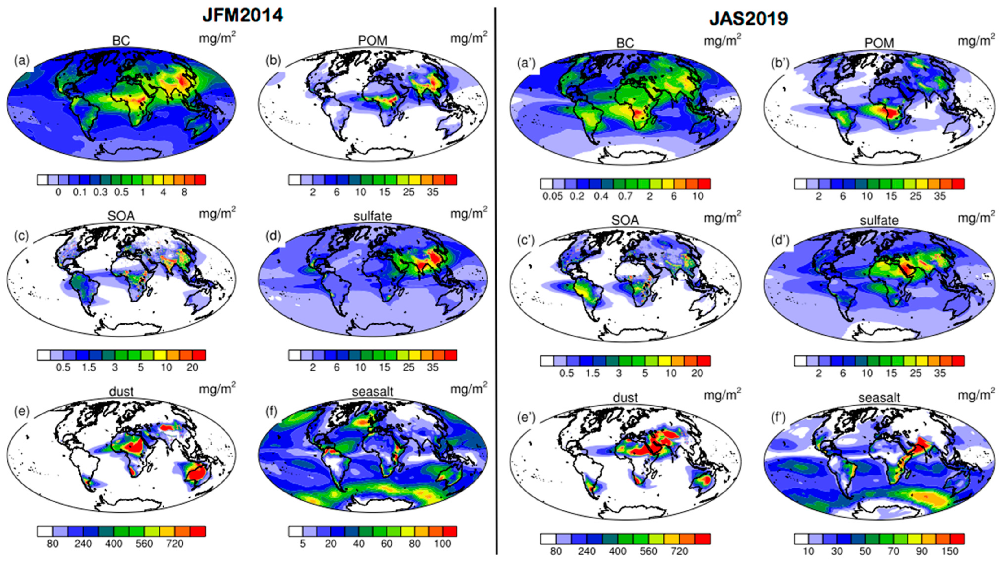
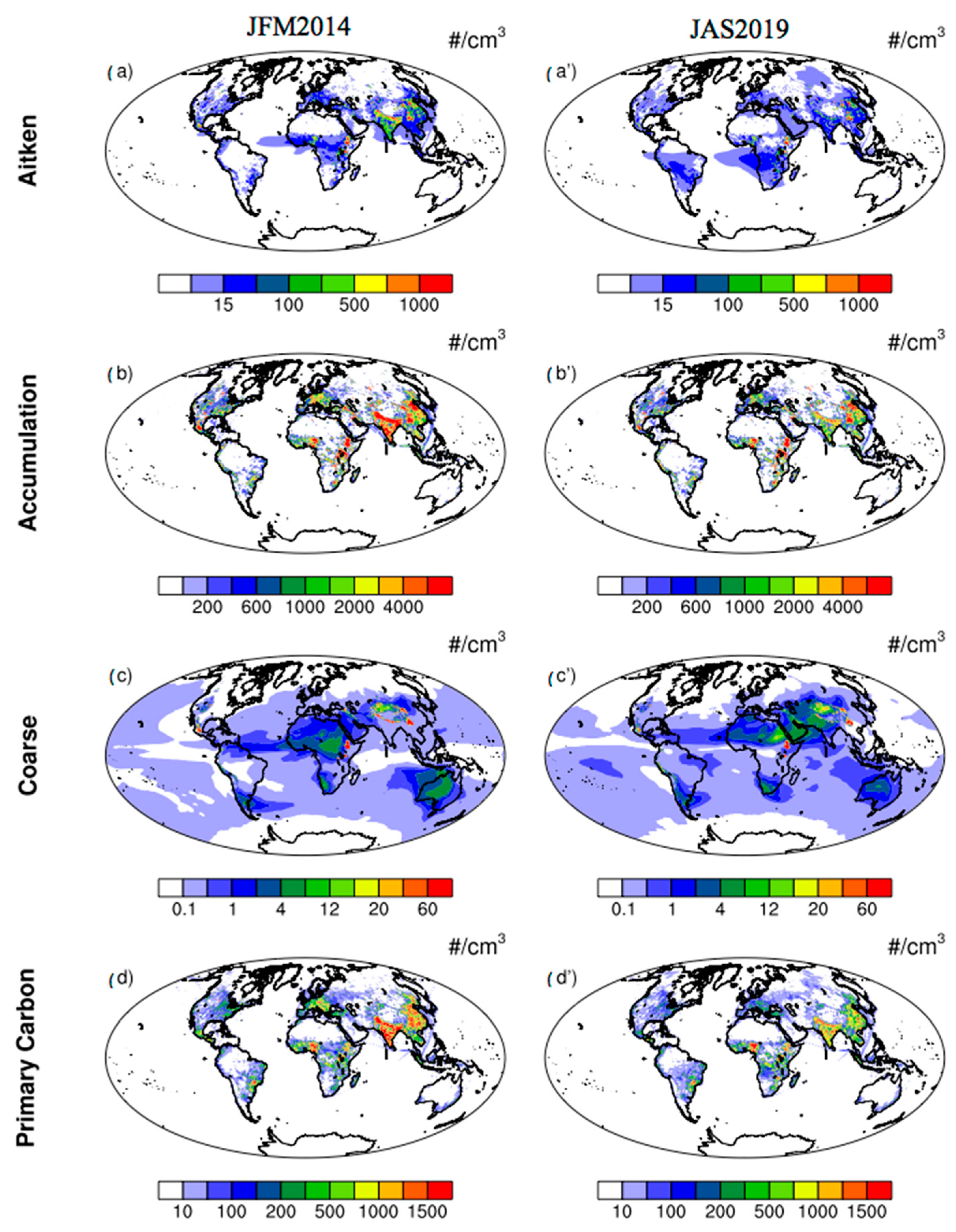
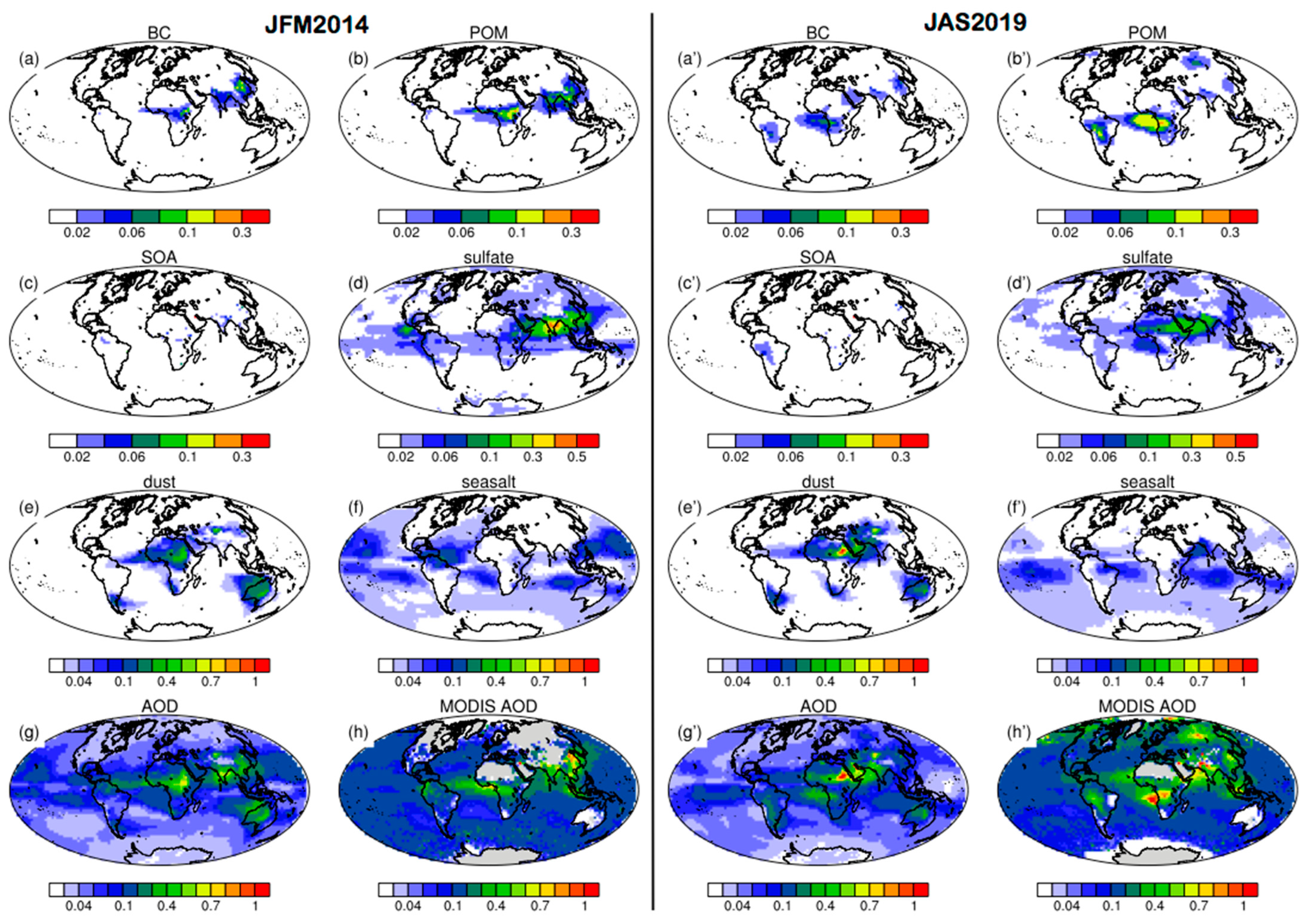
4.1. Global Aerosol Distributions

Figure 2 shows the mean total column mass concentrations of MAM4 species summed over the modes for JFM2014 and JAS2019. For example, concentrations of BC are from accumulation and primary carbon modes. Table 2 gives the global minima, maxima, and mean concentrations. Maximum BC concentrations (>8 mg/m2) are observed over the industrial areas in East Asia and biomass burning region in Central Africa in JFM2014. Moderate concentrations of about 0.5 to 6.0 mg/m2 are observed over South Asia, Europe, Southeast SA, North America, Northern SA, and Central Asia. Similar magnitudes are observed for POM distributions, except for larger contributions of POM over the regions where maximum BC concentrations are seen. For JAS2019, higher BC and POM concentrations are seen over the regions of intense biomass burning in SA and Africa, but comparatively, their concentrations are reduced over East Asia and Central Africa. Relatively, the concentrations over land masses in the northern hemisphere (NH) are also found to be increased. The intense biomass burning occurring in the southern hemisphere (SH) significantly contributes about a 40% increase in global POM concentrations and a 21% in global BC concentrations (Table 2). The 2019 biomass-burning season was one of the most intense biomass-burning seasons observed in over 20 years [42]. In the four-mode configuration, BC and POM are treated in accumulation and primary carbon modes. The explicit treatments for the ageing of carbonaceous particles to accumulation mode and the number of sulfate monolayers for ageing (equal to eight, here) result in an increased concentrations of BC and POM and increased residing time of BC in the primary carbon mode, allowing transport to remote regions, viz Pacific and Atlantic oceans and Arctic. The concentrations are very low over the high latitudes in the SH. Their strong seasonal variability over the biomass burning regions and modest response over industrial regions are also observed in other global models [61,100,101,102]. Similar to BC, SOA concentrations are higher over industrial areas and regions of high biogenic emissions. For the wet season in SA (in JFM2014), the SOA concentrations are relatively low, but they are otherwise higher in East Asia and Southeast Asia. Over higher latitudes in the NH, SOA concentrations are enhanced in JAS2019. Despite seasonal variations, global mean concentrations are similar (<5%).
Sulfate is produced from the oxidation of SO2. AMIC treats sulfate in accumulation, Aitken, and coarse modes. Sulfate is disseminated over the entire globe, with concentrations varying from 2 mg/m2 to over 40 mg/m2 and exhibiting strong seasonality. Over the anthropogenic source regions of East Asia, South Asia, and North America, sulfate concentrations are higher in JFM2014 and lower in JAS2019. The difference in the seasonal global mean is within 10%. The highest concentrations (>700 mg/m2) of mineral dust are observed over the source regions—North China and Arabian Peninsula in Asia, the Sahara, and arid regions in Africa, Western Australia, and southern part of SA. Seasonal variations are observed over source regions in Asia, SA, Southern Africa, and Australia, but high emissions from the Sahara are observed in both seasons. In Oceania, strong wind erosion occurs over the northern and northwestern parts of the continent, driving the emissions, which gradually shift towards the south. The simulations are able to reproduce the latitudinal shift of Saharan dust emissions modulated by the Inter Tropical Convergence Zone (ITCZ), as well as their transport towards the Caribbean and Northeast Brazil. This is consistent with other studies [22,26,61]. In AMIC, SS is treated in three modes: accumulation, Aitken, and coarse. Higher concentrations are associated with regions of strong wind speeds. In both seasons, concentrations exceeding 50 mg/m2 are observed in high latitudes in the North Atlantic, North Pacific, and oceans in the SH. Higher concentrations (>100 mg/m2) are also seen in the South Asia and Northern SA due to strong winds. Northern midlatitudes exhibit stronger seasonal variation compared to SH, corresponding to stronger and weaker wind-speed variability.
The mean number concentrations in the Aitken, accumulation, coarse, and primary carbon mode in the surface layer for both seasons are shown in Figure 3. In all the modes, surface concentrations are highest over primary emissions associated with biomass burning and anthropogenic activity. Overall, the number concentrations in the accumulation mode are higher over continents, which can be a result of the growth of the Aitken mode particles to accumulation mode, and the primary emission of BC, POM, and sulfate particles into the accumulation mode. Concentrations are much lower over oceans, while they exceed 4000 cm−3 over industrial areas in East Asia, South Asia, North America, and Europe, and over biomass burning regions in Central Africa. Moderate concentrations up to 2000 cm−3 are observed over Southeast Brazil, the Northeast United States (US), South Asia, and Europe during JAS 2019. Aitken mode number concentrations are higher over industrial regions with high sulfur emissions, but very low over biomass burning regions. For JAS2019, concentrations <50 cm−3 are observed over the Amazon and Southern Africa. Moderate concentrations up to 50 cm−3 are seen over India and East Asia during JFM2014. Coarse mode comprises of sulfate, DU, and SS. Concentrations up to 12 cm−3 over dust-source regions and 4 cm−3 over the outflow areas are seen in Figure 3c,c’. For the primary carbon mode, maximum concentrations up to 500 cm−3 are seen over the biomass burning regions of Central Africa and Central SA.

4.2. Cloud Microphysical Properties

We have examined the framework of AMIC in BAM subjected to the incoming emissions and forcings in Figure 2 and Figure 3. The BAM AMIC simulated mean cloud microphysical properties, namely vertically integrated column droplet number concentration and CCN at 0.5% supersaturation, for both the seasons are shown in Supplementary Figures S1 and S2, respectively. For JFM2014, concentrations above 2.5 × 10⁶ m−2 are seen over Europe and parts of Western Russia, followed by North America and Canada. Moderate concentrations in regions over the ocean at high latitudes in both hemispheres can be attributed to SS emissions due to high wind speeds. For JAS2019, concentrations up to 7 × 10⁵ m−2 are seen over SA, i.e., over the Amazon, eastern part of Brazil, and Southeast SA. Increased CDNCs are observed over Central India and the Arabian Sea during this period, which is the rainy season over the subcontinent. Maximum CCN concentrations are observed over regions with high emissions of carbonaceous and secondary organic aerosols, i.e., over the industrial and populated areas, biomass-burning regions, and along their outflows or downwind paths. CCN concentrations over SA peak over La Plata basin, which stretches from Northeastern Argentina to South–Southeastern Brazil and receives heat, moisture, and biomass burning products from the Amazon all year. As a consequence, destructive hailstorms are often observed over this mountainous region during late winter and early spring, between September and October [103]. An evaluation of BAM CTRL and BAM AMIC simulated shortwave COD, cloud fraction, and cloud LWP with MODIS observations for both the seasons are shown in Supplementary Figure S3a,b. The cloud fraction is significantly overpredicted in all the experiments, specifically over the higher latitudes in both hemispheres that can relate to higher CDNCs simulated over those regions. Following cloud fraction, shortwave COD is largely overpredicted, while the cloud LWP is significantly underpredicted.

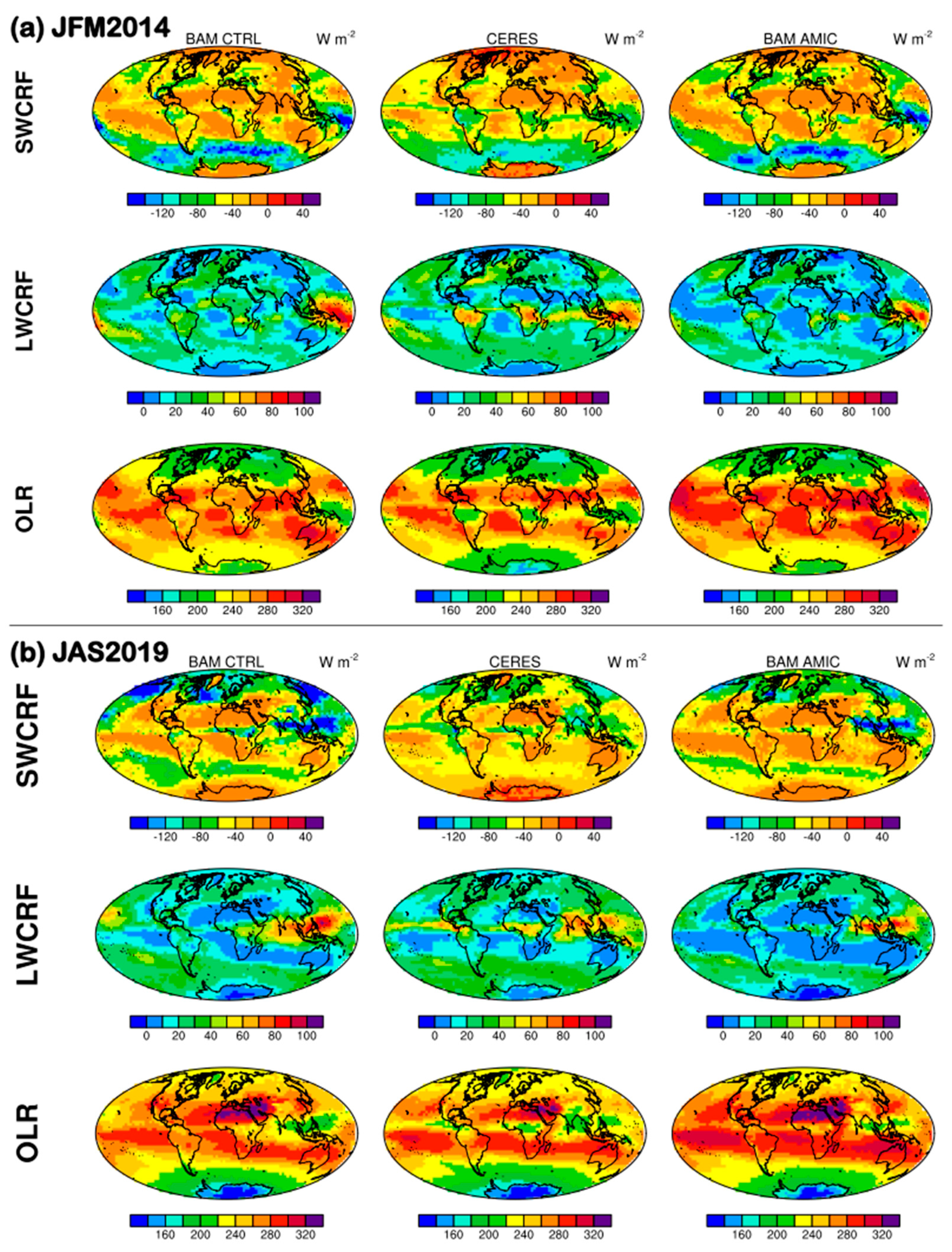
4.3. Cloud Radiative Properties

Simulated cloud radiative forcings (in W m−2) compared with observations from the CERES satellite are shown in Figure 4a,b, following a similar layout, and the model performance is summarized in Table 3 and Table 4. The simulated LW and SW forcing is calculated by subtracting forcing due to cloudy sky from forcing due to clear sky. The variables compared include shortwave cloud radiative forcing (SWCRF), longwave cloud radiative forcing (LWCRF), and outgoing longwave radiation (OLR). The downward shortwave (SWDOWN) radiation is shown in Supplementary Figure S4. For JFM2014 (Figure 4a), simulations without and with aerosols overpredict SWCRF. The observed global mean SWCRF is −40.66 W m−2, while the BAM CTRL and BAM AMIC simulated means are −43.98 and −45.15 W m−2, with an NMB of 8% and 11%, an RMSE of 20.91 and 22.26 W m−2, and an R of 0.84 and 0.82, respectively. Over the southern oceans, comparatively strong cooling is related to SS emissions that scatter light. In the tropics, where absorbing aerosols are higher, the cooling is relatively weak. Simulated LWCRF is underpredicted in both experiments. The observed global mean LWCRF is 22.08 W m−2, while the BAM CTRL and BAM AMIC simulated means are 19.24 and 15.96 W m−2, respectively, with an NMB of −13% and −28%, an RMSE of 10.57 and 11.23 W m−2, and an R of 0.72 and 0.76, respectively.
Over the Amazon and Central Africa, simulations underestimate, and other differences lie over the oceans. Strong overprediction is seen in the simulated SWDOWN radiation over the tropics and midlatitudes. The CERES observations yield a global average of 166.6 W m−2, and simulations yield 267 and 264 W m−2, respectively, for BAM CTRL and BAM AMIC. The sensitivity to the inclusion of aerosols is little. The NMBs are 60% and 58%, respectively, with RMSEs of 1261.1 and 122.9 W m−2. The OLR is overpredicted, with NMBs of 6% and 7.4%, respectively, for simulations without and with aerosols, and it represents poorly over the Amazon and Central Africa. During the biomass burning period in the SH (in the JAS2019 set of experiments), cooling is weak over peak regions. Figure 4b shows overprediction of SWCRF with an observed global mean −38.5 W m−2 and a simulated mean of −55.6 and −42 W m−2, respectively, for the BAM CTRL and BAM AMIC experiments. The NMBs indicate an improvement in the prediction of SWCRF due to the inclusion of aerosols. The SWDOWN shows similar characteristics in both seasons, with higher values over the tropics and midlatitudes. The LWCRF is underpredicted, with NMBs of −10% and −30% and RMSEs of 10.3 and 11 W m−2. The spatial patterns of the simulated OLR are mostly similar in both experiments and are overpredicted with global averages of 236.8 and 243 W m−2, respectively, for conditions without and with aerosols, compared to the observed value of 228.9 Wm−2.

4.4. Aerosol Optical Depth

The simulated total AOD at 550 nm for the periods JFM2014 and JAS2019 compared with the MODIS AOD product is shown in Figure 5 (bottom panel). For JAS2019, when biomass burning is at its peak in the Amazon and Central Africa, spatial patterns of AOD variations are captured in the simulations over these regions, though they are underpredicted. Over the Amazon, MODIS AOD values vary in the range of 0.4–0.6, and the simulated values are moderate (about 0.3); and the difference is much wider over Central Africa. Overall, the simulated AOD is strongly underpredicted, with a MODIS mean of 0.18 compared to the simulated 0.08. NMBs is −58% with RMSE 0.16 and R 0.42. High AOD values are seen over Northern Africa and near the Middle East. Incorporating detailed aerosol processes and aerosol inputs can reduce the bias. For instance, a biomass burning module, such as the most recent Brazilian Biomass Burning Emission Model, could replace the need to use background concentrations from CAM–Chem and improve the simulated AOD.
Spatial patterns over the outflow areas in the tropical Atlantic are captured. Over the Indian region, AOD is moderately predicted, but it is very low over East Asia. Figure 5 (top three rows) also shows simulated AOD explicitly due to AODBC, AODPOM, AODSOA, sulfate (AODsu), AODDU, and AODSS. Over the Amazon, significant contribution is from POM emissions with AODPOM ≈ 0.2, followed by AODBC ≈ 0.05 and AODSOA ≈ 0.04. Over Central Africa, AODPOM ≈ 0.3, followed by AODBC ≈ 0.1 and AODsu ≈ 0.08. Over strong dust source regions, AODDU ≈ 0.6 (Middle East), ≈ 1.0 (Sahara Desert) ≈ 0.16 (Southern SA). Over East Asia, sulfate dominates AODsu ≈ 0.08, followed by BC and POM. Over the oceans, SS contributes up to 0.08. For the JFM2014 period, there is a strong underprediction with NMB = –39%. The simulated patterns agree with observations over India, Central Africa, and the tropical Atlantic, where dust is transported from the Sahara towards SA. Over East Asia, MODIS observations show high values compared to simulated (≈ 0.6). Observed AODs over oceans range from 0.08 to 0.2, while the simulations vary between 0.02 and 0.1. Among the species, contributions of dust and sulfate are significant, with maximum AODsu ≈ 0.5 (South India and Southeast Asia) and AODDU ≈ 0.4 (Central Africa and Australia). The maximum contribution of POM and BC varies between 0.1 and 0.3.

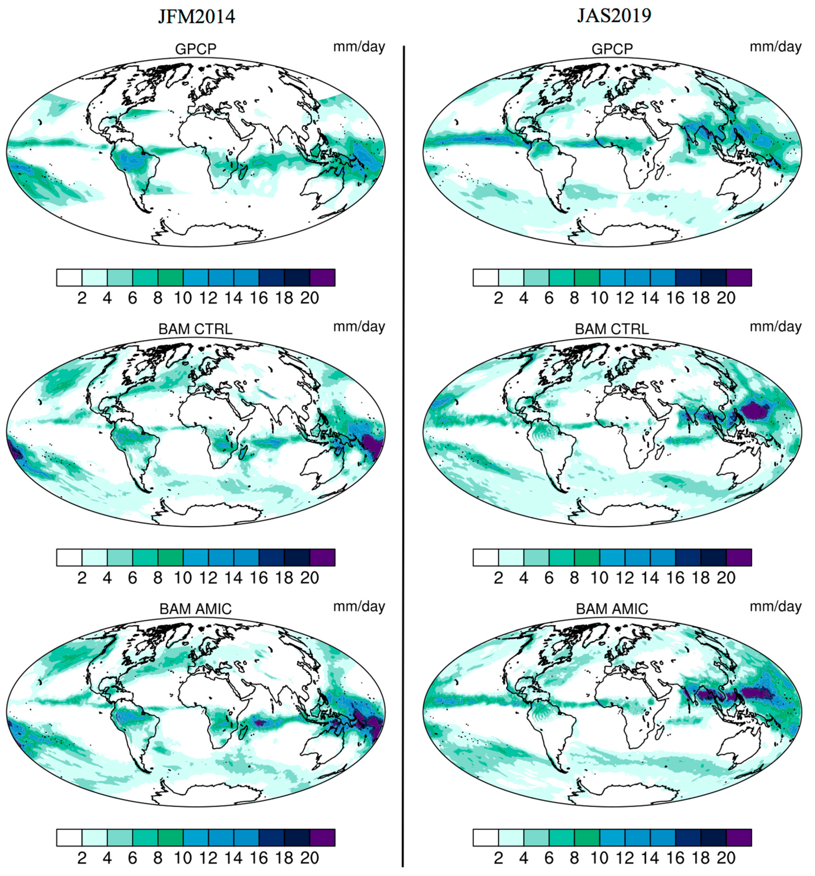
4.5. Other Atmospheric Variables
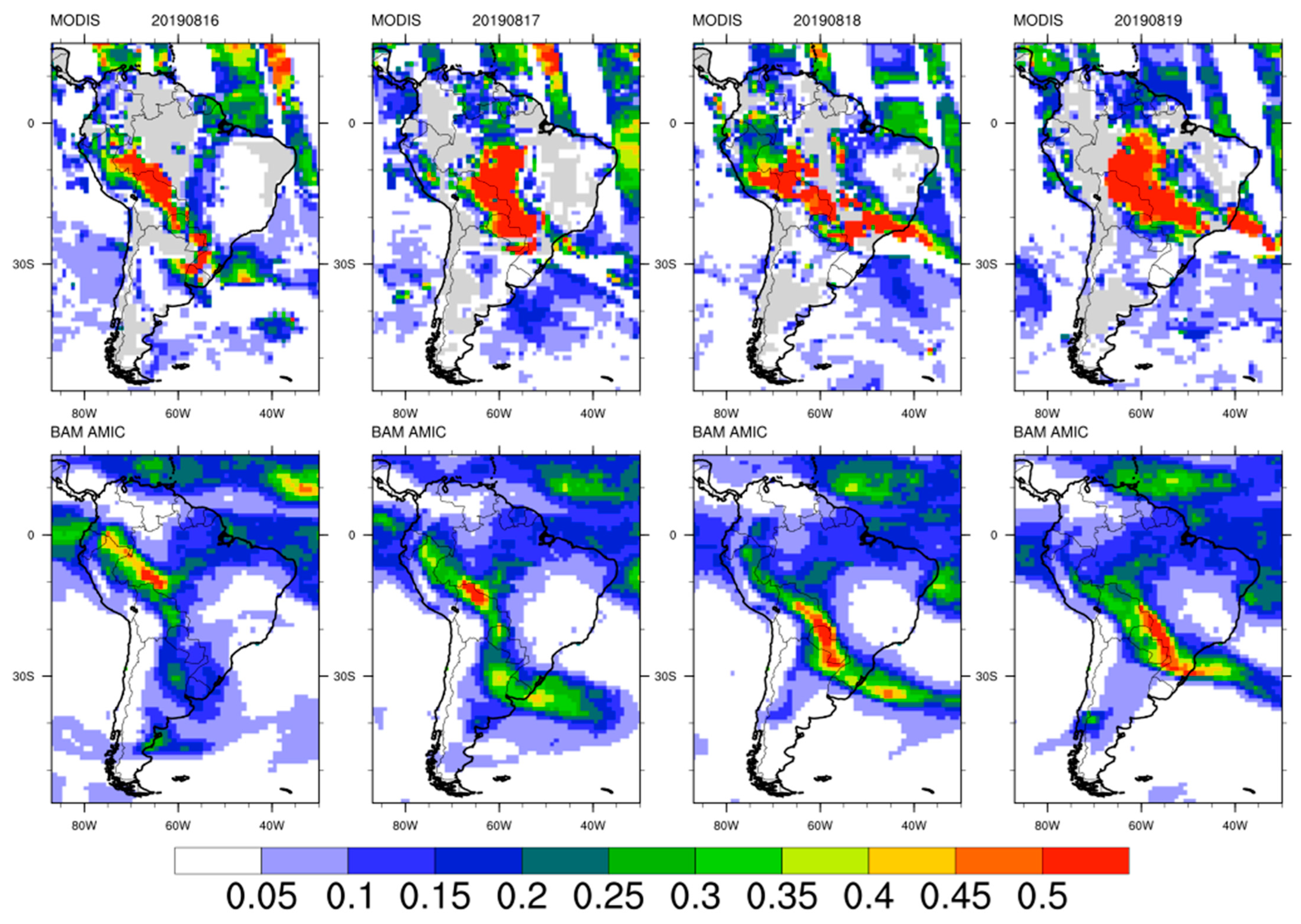
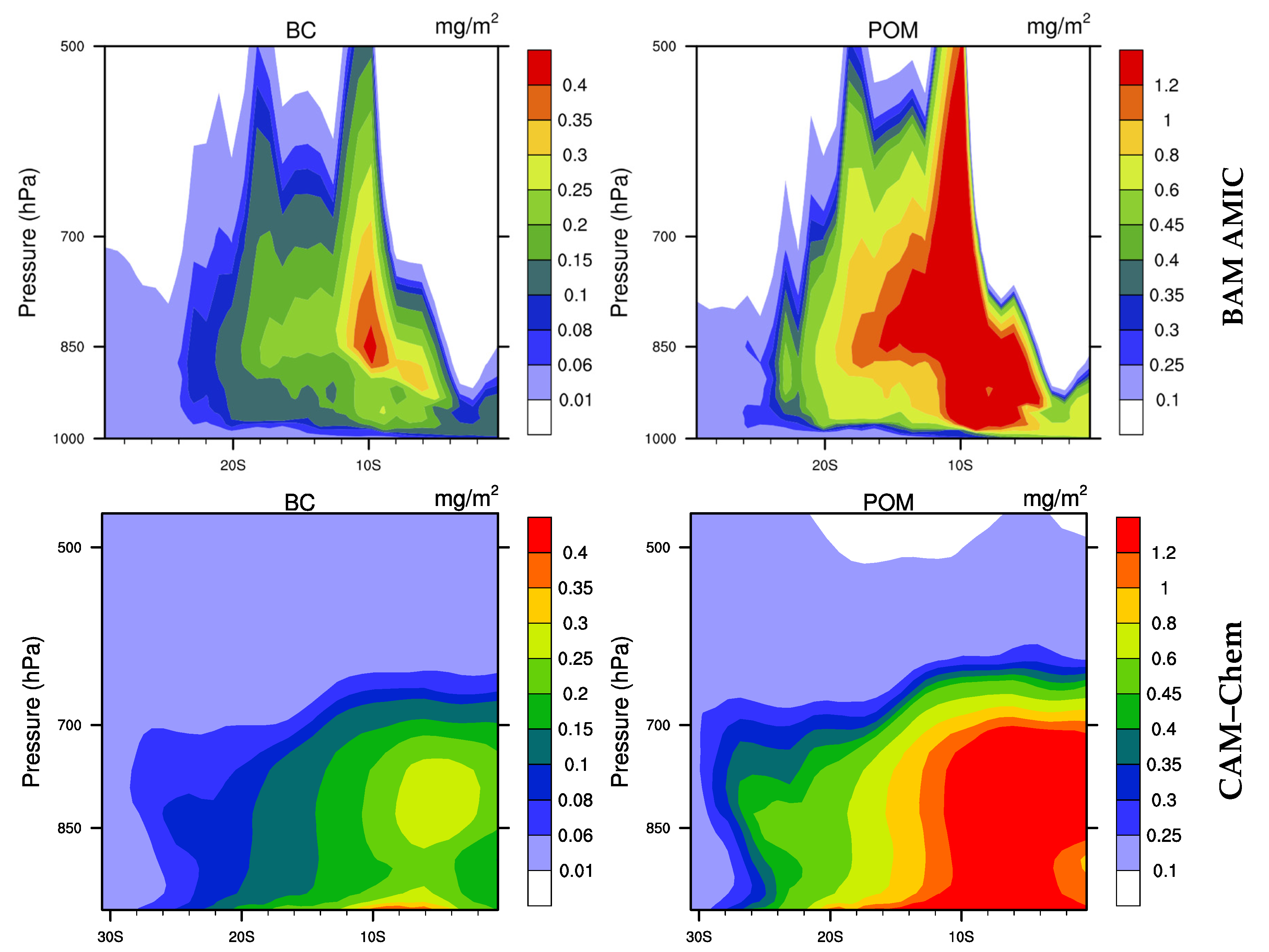
Precipitation features simulated in BAM CTRL and BAM AMIC for both sets of experiments, along with GPCP daily precipitation, are shown in Figure 6. For the JFM2014 set, which is a wet season in SA, precipitation over the La Plata basin is strongly underpredicted and moderately overpredicted over the South Atlantic Convergence Zone. Over Southern Africa and the Amazon basin, relatively, the simulated precipitation with aerosol included is slightly better. A strong overprediction is observed over the South Pacific. Moderate overprediction is seen over the high latitudes in the NH. Overall, both BAM CTRL and BAM AMIC simulations overpredict with NMBs of 85% and 97% and RMSE of 3.39 and 3.55, respectively (Table 3). In JAS2019 experiments, precipitation over the Indian continent is not well reproduced, and extreme values are observed over the equatorial West Pacific. However, the global means show good agreement with the observations. The NMB is 7% for BAM CTRL, with an RMSE of 3.72; and 14% for BAM AMIC, with an RMSE of 3.85 (Table 4).
Comparing the 2 m temperature simulated in BAM CTRL and BAM AMIC simulations, the inclusion of aerosols slightly increased the temperatures over equatorial and midlatitudes in both seasons (Supplementary Figure S5). On the contrary, 2 m specific humidity is reduced, leading to drier conditions due to the presence of aerosols.

4.6. Case Study

Biomass burning in the Amazon during the dry season has witnessed unprecedented increase in recent years. Mesoscale dynamical systems transport aerosol particles downwind towards populated areas, impacting regional weather [43,46]. August 2019 is considered the worst biomass burning season in the Amazon, during which smoke from the Amazon is transported down south, causing darkness over Sao Paulo during the daytime. Using the new CPTEC–WRF–Chem modeling framework, Vara-Vela et al. [42] reported a case study predicting the arrival of smoke down Southeast. As noted above, BAM is an operation model in CPTEC. In order to test the performance of BAM AMIC for an extreme aerosol-loading scenario, we ran a short BAM AMIC experiment following the configuration in Table 1 for the period 13–22 August 2019. The meteorological initial conditions and prescribed weekly sea surface temperature are generated for 13 August 12:00:00. Figure 7 shows the evaluation of the simulated daily averaged AOD 550 nm over SA against MODIS observations during the period 16–19 August. Relatively, the simulated AOD magnitude is lower but the model reproduces the spatial distribution from Central Amazon towards Southeast. Comparing the results with Figure 3 of the reported study [42], performance of BAM AMIC can be improved by incorporating treatment of fires in BAM and use of real-time fire products. The CPTEC–WRF–Chem modeling system performs as good as the ECMWF–Copernicus Atmosphere Monitoring Service owing to the use of near-real-time remote-sensing fire products.
Figure 8 compares the BAM AMIC simulated and CAM–Chem generated vertical distribution of zonally averaged mass concentrations of BC and POM during 15–22 August 2019, over latitudes 30° S–0°. Both models show biomass burning plumes being transported towards southern regions, with CAM–Chem showing more uniform distribution of aerosols with latitudes between 0° and 14° S, while in BAM AMIC, the plumes are restricted to a region between 6° and 14° S. However, the estimated burned area retrieved from satellite fire products shows comparatively much less fires over latitudes between 0° and 6° S for August 2019 (Supplementary Figure S1 in [42]), thereby indicating that the aerosol plumes are more realistically represented in BAM AMIC simulations [104]. Moreover, the BC and POM emissions are uplifted (surface level concentrations are 30–50% lower in emission areas compared to upper levels in the lower troposphere) and transported down south, thus indicating that BAM with aerosol parameterization is able to simulate advection and vertical mixing (Figure 8).

5. Conclusions

The preliminary results of the ongoing implementation of online-coupled aerosol interactions in global BAM were presented. The aerosol–chemistry–climate is a complex tightly coupled system that requires accurate representation of the mechanisms and feedbacks in a GCM. Several independent evaluation studies reported biases in representing climate over SA, and models differ widely in estimating the direct and indirect radiative forcings due to aerosols. Modeling centers such as PNNL, NCAR, and ECMWF have invested years of continued research in building state-of-the-science global aerosol–chemistry–climate models. From the implementation standpoint, it can be conjectured that significant modification is required in a GCM for the coupling. Realizing the humongous efforts required, CPTEC’s approach involves adopting a simplified aerosol module from NCAR in BAM rather than developing a better aerosol model, and subsequently extending it to include more complex aerosol processes. As seen from Supplementary Table S1, the online-coupled mode of interactions between aerosols and GCM treats the feedback mechanism in totality, providing a more realistic representation. The aerosol module is a microphysical subset of CAM–MAM that prognostically treats six aerosol species, namely BC, POM, SOA, sulfate, dust, and sea salt, partitioned into different lognormally distributed modes (seven-mode, four-mode, or three-mode) and computes aging, condensation, coagulation, nucleation, and renaming. A comparative study on the impacts of aerosol size distribution on aerosol–cloud interaction, using the modal (with both fixed and varying σg) and sectional approach in a single column version of this module in MIRAGE, has shown good agreement between the modal and sectional partitioning [105]. The module has been ported to BAM in an online-coupled mode and has been expanded to include feedback to Morrison double moment cloud microphysics and radiation schemes. A physically based treatment for aerosol activation [81], along with vertical mixing and CCN at different supersaturations, was implemented. Aerosol optical properties based on the Mie theory of scattering were computed. We note that, for the partial representation of aerosol processes implemented in BAM until now, we relied heavily on remote-sensing observations for model evaluation. Comparing with previous results from existing global aerosol models requires a complete representation of aerosol processes in BAM and is not viable or conclusive at the current stage of implementation. Therefore, the BAM global simulations are compared with satellite observations, which provide global data.
To assess the performance of the new parameterization, experiments without and with aerosols for two different periods, namely JFM 2014 and JAS 2019, were performed and evaluated by using satellite-based observations from MODIS, CERES, and GPCP. Firstly, the column integrated mass and number concentrations of the aerosol species were examined to understand the simulated distribution of aerosols in response to the inputs. Overall, the imprint of the intense biomass burning events in the Amazon is seen in the simulations [106,107]. BC, POM, sulfate, and dust species exhibit varying degrees of seasonality. The simulated spatial patterns are as expected from other studies. For instance, the latitudinal shift of Saharan dust emissions modulated by the ITCZ is captured in simulations. Similarly, BC and POM emissions from the biomass burning and their transport downwind are fairly simulated, as well. On the other hand, biogenic emissions over the Amazon and high sea salt emissions over the north and northwest of India are not well represented. The simulated seasonal variations in CDNC and CCN at 0.5% supersaturations are relatable to the distribution of mass and number concentrations. The indirect effect of aerosols is very sensitive to the aerosol activation scheme. Studies have shown improvement in CDNC and CCN predictions from using more detailed activation schemes in place of AG00, but they have also reported an increase in the computational times [108,109]. The model simulates aerosol optical depth as an integral, as well as for individual species. Relating to the mass and number distributions, over biomass burning and outflow regions, desert and arid regions, and industrial areas, the AODs are modestly simulated. AOD is underpredicted in both the seasons with NMBs −39% and −58% for JFM 2014 and JAS 2019, respectively. Simulated cloud properties, such as shortwave cloud optical depth, cloud fraction, and cloud liquid water, path have shown significant departures from MODIS data. The simulated cloud fraction in the experiment with no aerosols has a large positive bias and can be related with strong overpredictions of other variables. Experiments with aerosols increased the bias, leading to large deviations from observations. The simulated shortwave radiative forcing and outgoing longwave radiation have acceptable over-predictabilities with NMB ≤ 10%, while the longwave cloud radiative forcing is underpredicted with NMB ≤ −30. A short 10-day experiment simulating the 15–22 August 2019 intense biomass burning event, which resulted in the transport of smoke plumes down Southeast SA, was performed. BAM AMIC could reproduce the spatial pattern of the transport of aerosol particles emanating from Central Amazon on 16 August towards the southeast on 19 August. In addition, the vertical distribution of BC and POM over the Amazon and Southeast SA shows a realistic representation of vertical uplift and advection of smoke plumes towards the south. These results seen alongside CPTEC–WRF–Chem and ECMWF–CAMS predictions, and with BAM being an operational model in CPTEC, advocates for a future study to be performed to examine the predictability of BAM (with AMIC), with treatment of fires incorporated and usage of near-real-time fire products.
The current study is crucial for assessing the indirect effect simulated by the new parameterization before moving towards representing the complete aerosol life cycle in the Brazilian global model. Future work includes improving the cloud optical properties and implementing dry and wet deposition, scavenging, sulfur cycle, and other complex mechanisms to treat biomass burning aerosols, secondary organic aerosols, and volatile organic compounds.

Supplementary Materials

The supplementary information consists of Tables (S1 and S2) and 5 figures along with relevant text. The supplementary file can be downloaded at: https://www.mdpi.com/article/10.3390/rs15010278/s1. Table S1: Aerosol and their effects on climate; Table S2: List of acronyms; Figure S1: Vertically integrated column droplet number concentration (per m2) averaged for the periods–(a) JFM2014 and (b) JAS2019 in BAM AMIC experiments; Figure S2: Surface concentration (per cm3) of CCN at 0.5% supersaturation averaged for the periods–(a) JFM2014 and (b) JAS2019 in BAM AMIC experiments; Figure S3a: Model evaluation of cloud optical properties for JFM2014; Figure S3b: Model evaluation of cloud optical properties for JAS2019; Figure S4: Model evaluation of downward shortwave radiation for JFM2014 and JAS2019; Figure S5: 2-m temperature (top panel) and specific humidity (bottom panel) in BAM CTRL and BAM AMIC simulations averaged for the periods–JFM2014 and JAS2019.

Author Contributions

Conceptualization, J.P., A.V.-V., R.P.M.K., S.N.F. and D.L.H.; methodology, J.P., D.S., R.P.M.K. and A.V.-V.; software, J.P., S.N.F. and P.Y.K.; validation, J.P., A.V.-V., D.S.A., E.P.V. and D.S.; formal analysis, J.P., A.V.-V. and D.S.; investigation, J.P., D.L.H., S.N.F. and E.P.V.; resources, D.L.H., S.N.F., P.Y.K., D.S.A., H.B.G. and P.N.; writing—original draft preparation, J.P., S.N.F., R.P.M.K. and A.V.-V.; writing—review and editing, A.V.-V., S.N.F., D.S. and D.S.A.; visualization, J.P., A.V.-V. and D.S.; supervision, D.L.H., S.N.F., P.N., E.P.V. and H.B.G.; project administration, D.L.H., D.S.A. and H.B.G.; funding acquisition, D.L.H. All authors have read and agreed to the published version of the manuscript.

Funding

This research was funded by Coordination for the Improvement of Higher Education Personnel (CAPES, Brazil) through the project CAPES/Modelagem 88881.148662/2017-01, J.P. was funded by CAPES/Modelagem 88881.148662/2017-01 fellowship, and D.S. at Northeastern University, US, is supported by the Wellcome Trust Grant Number 216087/Z/19/Z (subaward #GR108374 from Yale University to Northeastern University).

Data Availability Statement

Not applicable.

Acknowledgments

We acknowledge Yang Zhang (Northeastern University), Richard Easter (PNNL), and X. Liu (University of Texas) for providing the aerosol module for BAM; Rebecca Buccholz (NCAR) and Simone Tilmes (NCAR) for providing CAM–Chem forcings for the experiments; the SDumont cluster in the National Laboratory for Scientific Computing (LNCC/MCTI, Brazil) for computational resources; and Coordination for the Improvement of Higher Education Personnel (CAPES, Brazil), National Council for Scientific and Technological Development (CNPq, Brazil). The EDGAR emissions were processed on the National Supercomputer TACC/NSF Stampede 2, provided as an Extreme Science and Engineering Discovery Environment (XSEDE) digital service by the Texas Advanced Computing Center (TACC) (http://www.tacc.utexas.edu, accessed on 19 November 2022), which is supported by National Science Foundation grant number ACI-1053575, and Cheyenne (doi:10.5065/D6RX99HX) provided by NCAR's Computational and Information Systems Laboratory, sponsored by the National Science Foundation.

Conflicts of Interest

The authors declare no conflict of interest.

References

  1. Haywood, J.; Boucher, O. Estimates of the direct and indirect radiative forcing due to tropospheric aerosols–A review. Rev. Geophys. 2000, 38, 513–543. [Google Scholar] [CrossRef]
  2. Twomey, S. Pollution and the planetary albedo. Atmos. Environ. 1974, 8, 1251–1256. [Google Scholar] [CrossRef]
  3. Twomey, S. Influence of pollution on shortwave albedo of clouds. J. Atmos. Sci. 1977, 34, 1149–1152. [Google Scholar] [CrossRef]
  4. Twomey, S. Aerosols, clouds and radiation. Atmos. Environ. 1991, 25A, 2435–2442. [Google Scholar] [CrossRef]
  5. Boucher, O.; Randall, D.; Artaxo, P.; Bretherton, C.; Feingold, G.; Forster, P.; Kerminen, V.-M.; Kondo, Y.; Liao, H.; Lohmann, U.; et al. Clouds and aerosols. In Climate Change 2013: The Physical Science Basis; Contribution of Working Group I to the Fifth Assessment Report of the Intergovernmental Panel on Climate Change; Stocker, T.F., Qin, D., Plattner, G.-K., Tignor, M., Allen, S., Boschung, J., Nauels, A., Xia, Y., Bex, V., Midgley, P., Eds.; Cambridge University Press: Cambridge, UK, 2013; pp. 571–657. [Google Scholar]
  6. Myhre, G.; Shindell, D.; Pongratz, J. Anthropogenic and Natural Radiative Forcing. In Climate Change 2013: The Physical Science Basis; Contribution of Working Group I to the Fifth Assessment Report of the Intergovernmental Panel on Climate Change; Stocker, T.F., Ed.; Cambridge University Press: Cambridge, UK, 2013. [Google Scholar]
  7. Masson-Delmotte, V.; Zhai, P.; Pirani, A.; Connors, S.L.; Péan, C.; Berger, S.; Caud, N.; Chen, Y.; Goldfarb, L.; Gomis, M.I.; et al. IPCC, 2021. In Climate Change 2021: The Physical Science Basis; Contribution of Working Group I to the Sixth Assessment Report of the Intergovernmental Panel on Climate Change; Cambridge University Press: Cambridge, UK; New York, NY, USA, 2021. [Google Scholar] [CrossRef]
  8. Zhang, Y. Online-coupled meteorology and chemistry models: History, current status, and outlook. Atmos. Chem. Phys. 2008, 8, 2895–2932. [Google Scholar] [CrossRef] [Green Version]
  9. Jacobson, M.Z. Strong radiative heating due to the mixing state of black carbon in atmospheric aerosols. Nature 2001, 409, 695–697. [Google Scholar] [CrossRef]
  10. Jacobson, M.Z. Control of fossil-fuel particulate black carbon plus organic matter, possibly the most effective method of slowing global warming. J. Geophys. Res. 2002, 107, 4410. [Google Scholar] [CrossRef] [Green Version]
  11. Chung, S.H.; Seinfeld, J.H. Climate response of direct radiative forcing of anthropogenic black carbon. J. Geophys. Res. 2005, 110, 1102. [Google Scholar] [CrossRef]
  12. Penner, J.E.; Zhang, S.Y.; Chuang, C.C. Soot and smoke aerosol may not warm climate. J. Geophys. Res. 2003, 108, 4657. [Google Scholar] [CrossRef]
  13. Feichter, J.; Lohmann, U.; Schult, I. The atmospheric sulphur cycle in ECHAM-4 and its impact on the shortwave radiation. Clim. Dyn. 1997, 13, 235–246. [Google Scholar] [CrossRef] [Green Version]
  14. Lohmann, U.; Feichter, J. Impact of sulfate aerosols on albedo and lifetime of clouds- A sensitivity study with the ECHAM GCM. J. Geophys. Res. 1997, 102, 13685–13700. [Google Scholar] [CrossRef]
  15. Kiehl, J.T.; Schneider, T.L.; Rasch, P.J.; Barth, M.C.; Wong, J. Radiative forcing due to sulfate aerosols from simulations with the NCAR community climate model. J. Geophys. Res. 2000, 105, 1441–1457. [Google Scholar] [CrossRef]
  16. Lohmann, U.; Feichter, J.; Penner, J.E.; Leaitch, R. Indirect effect of sulfate and carbonaceous aerosols: A mechanistic treatment. J. Geophys. Res. 2000, 105, 12193–12206. [Google Scholar] [CrossRef]
  17. Ghan, S.J.; Easter, R.C.; Chapman, E.G.; Abdul-Razzak, H.; Zhang, Y.; Leung, L.R.; Laulainen, N.S.; Saylor, R.D.; Zaveri, R.A. A physically based estimate of radiative forcing by anthropogenic sulfate aerosol. J. Geophys. Res. 2001, 106, 5279–5293. [Google Scholar] [CrossRef] [Green Version]
  18. Andreae, M.O.; Crutzen, P.J. Atmospheric aerosols: Bio-geochemical sources and role in atmospheric chemistry. Science 1997, 276, 1052–1058. [Google Scholar] [CrossRef] [Green Version]
  19. Spracklen, D.V.; Jimenez, J.L.; Carslaw, K.S.; Worsnop, D.R.; Evans, M.J.; Mann, G.W.; Zhang, Q.; Canagaratna, M.R.; Allan, J.; Coe, H.; et al. Aerosol mass spectrometer constraint on the global secondary organic aerosol budget. Atmos. Chem. Phys. 2011, 11, 12109–12136. [Google Scholar] [CrossRef] [Green Version]
  20. Scott, C.E.; Rap, A.; Spracklen, D.V.; Forster, P.M.; Carslaw, K.S.; Mann, G.W.; Pringle, K.J.; Kivekäs, N.; Kulmala, M.; Lihavainen, H.; et al. The direct and indirect radiative effects of biogenic secondary organic aerosol. Atmos. Chem. Phys. 2014, 14, 447–470. [Google Scholar] [CrossRef] [Green Version]
  21. Shrivastava, M.; Cappa, C.D.; Fan, J.; Goldstein, A.H.; Guenther, A.B.; Jimenez, J.L.; Kuang, C.; Laskin, A.; Martin, S.T.; Ng, N.L.; et al. Recent advances in understanding secondary organic aerosol: Implications for global climate forcing. Rev. Geophys. 2017, 55, 509–559. [Google Scholar] [CrossRef] [Green Version]
  22. Prospero, J.M.; Glaccum, R.A.; Nees, R.T. Atmospheric transport of soil dust from Africa to South America. Nature 1981, 289, 570–572. [Google Scholar] [CrossRef]
  23. Perry, K.D.; Cahill, T.A.; Eldred, R.A.; Dutcher, D.D.; Gill, T.E. Long-range transport of North African dust to the eastern United States. J. Geophys. Res. 1997, 102, 11225–11238. [Google Scholar] [CrossRef]
  24. Meywerk, J.; Ramanathan, V. Observations of the spectral clear-sky aerosol forcing over the Tropical Indian Ocean. J. Geophys. Res. 1999, 104, 24359–24370. [Google Scholar] [CrossRef]
  25. Parrington, J.R.; Zoller, W.H.; Aras, N.K. Asian dust: Seasonal transport to the Hawaiian Islands. Science 1983, 220, 195–197. [Google Scholar] [CrossRef]
  26. Ginoux, P.; Chin, M.; Tegen, I.; Prospero, J.; Holben, B.; Dubovik, O.; Lin, S.J. Sources and distributions of aerosols simulated with the GOCART model. J. Geophys. Res. 2001, 106, 20255–20273. [Google Scholar] [CrossRef]
  27. Tegen, I.; Harrison, S.P.; Kohfeld, K.; Prentice, I.C.; Heimann, M. The impact of vegetation and preferential source areas on global dust aerosol: Results from a model study. J. Geophys. Res. 2002, 107, 4576. [Google Scholar] [CrossRef] [Green Version]
  28. Luo, C.; Mahowald, N.M.; del Corral, J. Sensitivity study of meteorological parameters on mineral aerosol mobilization, transport, and distribution. J. Geophys. Res. 2003, 108, 4447. [Google Scholar] [CrossRef] [Green Version]
  29. Miller, R.L.; Tegen, I.; Perlwitz, J. Surface radiative forcing by soil dust aerosols and the hydrologic cycle. J. Geophys. Res. 2004, 109, D04203. [Google Scholar] [CrossRef]
  30. Zender, C.S.; Miller, R.L.; Tegen, I. Quantifying mineral dust mass budgets: Systematic terminology, constraints, and current estimates. Eos Trans. AGU 2004, 85, 509–512. [Google Scholar] [CrossRef]
  31. Woodward, S. Modeling the atmospheric life cycle and radiative impact of mineral dust in the Hadley Centre climate model. J. Geophys. Res. 2001, 106, 18155–18166. [Google Scholar] [CrossRef] [Green Version]
  32. Miller, R.L.; Cakmur, R.V.; Perlwitz, J.; Geogdzhayev, I.V.; Ginoux, P.; Koch, D.; Kohfeld, K.E.; Prigent, C.; Ruedy, R.; Schmidt, G.A.; et al. Mineral dust aerosols in the NASA Goddard Institute for Space Sciences ModelE atmospheric general circulation model. J. Geophys. Res. 2006, 111, D06208. [Google Scholar] [CrossRef]
  33. Yoshioka, M.; Mahowald, N.M.; Conley, A.J.; Collins, W.D.; Fillmore, D.W.; Zender, C.S.; Coleman, D.B. Impact of Desert Dust Radiative Forcing on Sahel Precipitation: Relative Importance of Dust Compared to Sea Surface Temperature Variations, Vegetation Changes, and Greenhouse Gas Warming. J. Clim. 2007, 20, 1445–1467. [Google Scholar] [CrossRef]
  34. Blanchard, D.C. The Production, Distribution, and Bacterial Enrichment of the Sea-Salt Aerosol. In Air-Sea Exchange of Gases and Particles; Liss, P.S., Slinn, W.G.N., Reidel, D., Norwell, M., Eds.; Springer: Dordrecht, The Netherlands, 1983; pp. 407–454. [Google Scholar]
  35. Monahan, E.C.; Spiel, D.E.; Davidson, K.L. A Model of Marine Aerosol Generation Via Whitecaps and Wave Disruption. In Oceanic Whitecaps; Oceanographic Sciences Library Series; Monahan, E.C., Niocaill, G.M., Eds.; Springer: Dordrecht, The Netherlands, 1986; Volume 2. [Google Scholar] [CrossRef]
  36. Erickson, D.J.; Duce, R.A. On the global flux of atmospheric sea salt. J. Geophys. Res. 1988, 93, 14079. [Google Scholar] [CrossRef]
  37. Gong, S.L.; Barrie, L.A.; Prospero, J.; Savoie, D.L.; Ayers, G.P.; Blanchet, J.-P.; Spacek, L. Modeling sea-salt aerosols in the atmosphere, Part 2: Atmospheric concentrations and fluxes. J. Geophys. Res. 1997, 102, 3819–3830. [Google Scholar] [CrossRef] [Green Version]
  38. Gong, S.L.; Barrie, L.A.; Blanchet, J.-P. Modeling sea-salt aerosols in the atmosphere: 1. Model development. J. Geophys. Res. 1997, 102, 3805–3818. [Google Scholar] [CrossRef] [Green Version]
  39. Artaxo, P.; Martins, J.V.; Yamasoe, M.A.; Procopio, A.S.; Pauliquevis, T.M.; Andreae, M.O.; Guyon, P.; Gatti, L.V.; Leal, A.M.C. Physical and chemical properties of aerosols in the wet and dry season in Rondonia, Amazonia. J. Geophys. Res. 2002, 107, 8081e8095. [Google Scholar] [CrossRef]
  40. Artaxo, P.; Rizzo, L.V.; Brito, J.F.; Barbosa, H.M.J.; Arana, A.; Sena, E.T.; Cirino, G.G.; Bastos, W.; Martin, S.T.; Andreae, M.O. Atmospheric aerosols in Amazonia and land use change: From natural biogenic to biomass burning conditions. Faraday Discuss. 2013, 165, 203–235. [Google Scholar] [CrossRef] [PubMed] [Green Version]
  41. Martin, S.T.; Andreae, M.O.; Artaxo, P.; Baumgardner, D.; Chen, Q.; Goldstein, A.H.; Guenther, A.; Heald, C.L.; Mayol- Bracero, O.L.; McMurry, P.H.; et al. Sources and properties of Amazonian aerosol particles. Rev. Geophys. 2010, 48, RG2002. [Google Scholar] [CrossRef] [Green Version]
  42. Vara-Vela, A.L.; Herdies, D.L.; Alvim, D.S.; Vendrasco, É.P.; Figueroa, S.N.; Pendharkar, J.; Reyes Fernandez, J.P. A New Predictive Framework for Amazon Forest Fire Smoke Dispersion over South America. Bull. Am. Meteorol. Soc. 2021, 102, E1700–E1713. [Google Scholar] [CrossRef]
  43. Freitas, S.R.; Longo, K.M.; Silva Dias, M.A.F.; Silva Dias, P.L.; Chatfield, R.; Prins, E.; Artaxo, P.; Grell, G.A.; Recuero, F.S. Monitoring the transport of biomass burning emissions in South America. Environ. Fluid Mech. 2005, 5, 135–167. [Google Scholar] [CrossRef]
  44. Andreae, M.; Artaxo, P.; Fischer, H.; Freitas, S.; Grégoire, J.-M.; Hansel, A.; Hoor, P.; Kormann, R.; Krejci, R.; Lange, L.; et al. Transport of biomass burning smoke to the upper troposphere by deep convection in the equatorial region. Geophys. Res. Lett. 2001, 28, 951. [Google Scholar] [CrossRef] [Green Version]
  45. Alvim, D.S.; Chiquetto, J.B.; D’Amelio, M.T.S.; Khalid, B.; Herdies, D.L.; Pendharkar, J.; Corrêa, S.M.; Figueroa, S.N.; Frassoni, A.; Capistrano, V.B.; et al. Evaluating Carbon Monoxide and Aerosol Optical Depth Simulations from CAM-Chem Using Satellite Observations. Remote Sens. 2021, 13, 2231. [Google Scholar] [CrossRef]
  46. Martins, L.D.; Hallak, R.; Alves, R.C.; de Almeida, D.S.; Squizzato, R.; Moreira, C.A.; Beal, A.; da Silva, I.; Rudke, A.; Martins, J.A. Long-range Transport of Aerosols from Biomass Burning over Southeastern South America and their Implications on Air Quality. Aerosol Air Qual. Res. 2018, 18, 1734–1745. [Google Scholar] [CrossRef] [Green Version]
  47. Gilardoni, S.; Di Mauro, B.; Bonasoni, P. Black carbon, organic carbon, and mineral dust in South American tropical glaciers: A review. Glob. Planet. Change 2022, 213, 103837. [Google Scholar] [CrossRef]
  48. Lamarque, J.-F.; Shindell, D.T.; Josse, B.; Young, P.J.; Cionni, I.; Eyring, V.; Bergmann, D.; Cameron-Smith, P.; Collins, W.J.; Doherty, R.; et al. The Atmospheric Chemistry and Climate Model Intercomparison Project (ACCMIP): Overview and description of models, simulations and climate diagnostics. Geosci. Model Dev. 2013, 6, 179–206. [Google Scholar] [CrossRef] [Green Version]
  49. Shindell, D.T.; Lamarque, J.-F.; Schulz, M.; Flanner, M.; Jiao, C.; Chin, M.; Young, P.J.; Lee, Y.H.; Rotstayn, L.; Mahowald, N.; et al. Radiative forcing in the ACCMIP historical and future climate simulations. Atmos. Chem. Phys. 2013, 13, 2939–2974. [Google Scholar] [CrossRef] [Green Version]
  50. Lee, Y.H.; Lamarque, J.-F.; Flanner, M.G.; Jiao, C.; Shindell, D.T.; Berntsen, T.; Bisiaux, M.M.; Cao, J.; Collins, W.J.; Curran, M.; et al. Evaluation of preindustrial to present-day black carbon and its albedo forcing from Atmospheric Chemistry and Climate Model Intercomparison Project (ACCMIP). Atmos. Chem. Phys. 2013, 13, 2607–2634. [Google Scholar] [CrossRef] [Green Version]
  51. Alvim, D.S.; Pendharkar, J.; Capistrano, V.B.; Frassoni, A.; Enoré, D.P.; Neto, O.L.D.M.; Gutierrez, E.R.; Choudhury, A.D.; Kubota, P.Y.; Da Silva, J.; et al. Aerosol distribution over Brazil with ECHAM-HAM and CAM5-MAM3 simulations and its comparison with ground-based and satellite data. Atmos. Pollut. Res. 2017, 8, 718–728. [Google Scholar] [CrossRef]
  52. Figueroa, S.N.; Bonatti, J.P.; Kubota, P.Y.; Grell, G.A.; Morrison, H.; Barros, S.R.M.; Fernandez, J.P.R.; Ramirez, E.; Siqueira, L.; Luzia, G.; et al. The Brazilian Global Atmospheric Model (BAM): Performance for tropical rainfall forecasting and sensitivity to convective scheme and horizontal resolution. Weather. Forecast. 2016, 31, 1547–1572. [Google Scholar] [CrossRef]
  53. Nobre, P.; Siqueira, L.S.P.; de Almeida, R.A.F.; Malagutti, M.; Giarolla, E.; Castelão, G.P.; Bottino, M.J.; Kubota, P.; Figueroa, S.N.; Costa, M.C.; et al. Climate Simulation and Change in the Brazilian Climate Model. J. Clim. 2013, 26, 6716–6732. [Google Scholar] [CrossRef]
  54. Capistrano, V.B.; Nobre, P.; Tedeschi, R.; Silva, J.; Bottino, M.; da Silva, M.B., Jr.; Menezes Neto, O.L.; Figueroa, S.N.; Bonatti, J.P.; Kubota, P.Y.; et al. Overview of climate change in the BESM-OA2.5 climate model. Geosci. Model Dev. 2018, 12, 1613–1642. [Google Scholar] [CrossRef] [Green Version]
  55. Veiga, S.F.; Nobre, P.; Giarolla, E.; Capistrano, V.; Baptista, M.; Marquez, A., Jr.; Figueroa, S.N.; Bonatti, J.P.; Kubota, P.; Nobre, C.A. The Brazilian earth system model version 2.5: Evaluation of its CMIP5 historical simulation. Geosci. Model Dev. 2019, 12, 1613–1642. [Google Scholar] [CrossRef] [Green Version]
  56. Guimarães, B.S.; Coelho, C.A.S.; Woolnough, S.J.; Kubota, P.Y.; Bastarz, C.F.; Figueroa, S.N.; Bonatti, J.P.; de Souza, D.C. Configuration and hindcast quality assessment of a brazilian global sub-seasonal prediction system. Q. J. R. Meteorol. Soc. 2020, 146, 1067–1084. [Google Scholar] [CrossRef]
  57. Cavalcanti, I.F.A.; Silveira, V.P.; Figueroa, S.N.; Kubota, P.Y.; Bonatti, J.P.; de Souza, D.C. Climate variability over South America-regional and large scale features simulated by the Brazilian Atmospheric Model (BAM-v0). Int. J. Climatol. 2019, 40, 2845–2869. [Google Scholar] [CrossRef]
  58. Coelho, C.A.S.; de Souza, D.C.; Kubota, P.Y.; Costa, S.; Menezes, L.; Guimarães, B.S.; Figueroa, S.N.; Bonatti, J.P.; Cavalcanti, I.F.; Sampaio, G.; et al. Evaluation of climate simulations produced with the Brazilian global atmospheric model version 1.2. Clim. Dyn. 2021, 56, 873–898. [Google Scholar] [CrossRef]
  59. de Souza, D.C.; Kubota, P.Y.; Figueroa, S.N.; Gutierrez, E.M.A.R.; Coelho, C.A.S. Impacto da resolução horizontal na simulação dos jatos de baixos níveis na América do Sul usando o modelo global do CPTEC. In Estudos Interdisciplinares nas Ciências Exatas e da Terra e Engenharias 4, E82 ed.; Atena Editora: Ponta Grossa, Brasil, 2019; pp. 205–217. [Google Scholar] [CrossRef] [Green Version]
  60. Guimarães, B.S.; Coelho, C.A.S.; Woolnough, S.J.; Kubota, P.Y.; Bastarz, C.F.; Figueroa, S.N.; Bonatti, J.P.; de Souza, D.C. An inter-comparison performance assessment of a Brazilian global sub-seasonal prediction model against four sub-seasonal to seasonal (S2S) prediction project models. Clim. Dyn. 2021, 56, 2359–2375. [Google Scholar] [CrossRef]
  61. Easter, R.C.; Ghan, S.J.; Zhang, Y.; Saylor, R.D.; Chapman, E.G.; Laulainen, N.S.; Abdul-Razzak, H.; Leung, L.R.; Bian, X.; Zaveri, R.A. MIRAGE: Model description and evaluation of aerosols and trace gases. J. Geophys. Res. Atmos. 2004, 109, D20210. [Google Scholar] [CrossRef]
  62. Liu, X.; Easter, R.C.; Ghan, S.J.; Zaveri, R.; Rasch, P.; Shi, X.; Lamarque, J.-F.; Gettelman, A.; Morrison, H.; Vitt, F.; et al. Toward a minimal representation of aerosols in climate models: Description and evaluation in the Community Atmosphere Model CAM5. Geosci. Model Dev. 2012, 5, 709–739. [Google Scholar] [CrossRef] [Green Version]
  63. Liu, X.; Ma, P.-L.; Wang, H.; Tilmes, S.; Singh, B.; Easter, R.C.; Ghan, S.J.; Rasch, P.J. Description and evaluation of a new four-mode version of the Modal Aerosol Module (MAM4) within version 5.3 of the Community Atmosphere Model. Geosci. Model Dev. 2016, 9, 505–522. [Google Scholar] [CrossRef]
  64. Morrison, G.; Curry, J.A.; Khvorostyanov, V.I. A new double-moment microphysics parameterization for application in cloud and climate models. Part I: Description. J. Atmos. Sci. 2005, 62, 1665–1677. [Google Scholar] [CrossRef]
  65. Iacono, M.; Delamere, J.; Mlawer, E.; Shephard, M.; Clough, S.; Collins, W. Radiative forcing by long-lived greenhouse gases: Calculations with the AER radiative transfer models. J. Geophys. Res. 2008, 113, D13103. [Google Scholar] [CrossRef]
  66. Tiedtke, M. The Sensitivity of the Time-Mean Large-Scale Flow to Cumulus Convection in the ECMWF Model. In Proceedings of the Workshop on Convection in Large-Scale Models, ECMWF, Reading, UK, 28 November–1 December 1983; pp. 297–316. [Google Scholar]
  67. Arakawa, A.; Schubert, W.H. Interaction of a cumulus cloud ensemble with the large-scale environment, Part I. J. Atmos. Sci. 1974, 31, 674–701. [Google Scholar] [CrossRef]
  68. Foley, J.A.; Prentice, I.C.; Ramankutty, N.; Levis, S.; Pollard, D.; Sitch, S.; Haxeltine, A. An integrated biosphere model of land surface processes, terrestrial carbon balance, and vegetation dynamics. Glob. Biogeochem. Cycles 1996, 10, 603–628. [Google Scholar] [CrossRef]
  69. Kucharik, C.J.; Foley, J.A.; Delire, C.; Fisher, V.A.; Coe, M.T.; Lenters, J.D.; Young-Molling, C.; Ramankutty, N.; Norman, J.M.; Gower, S.T. Testing the performance of a dynamic global ecosystem model: Water balance, carbon balance, and vegetation structure. Glob. Biogeochem. Cycles 2000, 14, 795–826. [Google Scholar] [CrossRef]
  70. Kubota, P.Y. Variability of Storage Energy in the Soil-Canopy System and its Impact on the Definition of Precipitation Standard in South America (in Portuguese with abstract in English). Ph.D. Thesis, Instituto Nacional de Pesquisas Espaciais (INPE), São José dos Campos, Brazil, 2012; 285p. [Google Scholar]
  71. Giorgi, F. Development of an Atmospheric Model for Studies of Global Budgets and Effects of Airborne Particulate Material. Ph.D. Thesis, The Georgia Institute of Technology, Atlanta, GA, USA, 1986. [Google Scholar]
  72. Ghan, S.J.; Laulainen, N.S.; Easter, R.C.; Wagener, R.; Nemesure, S.; Chapman, E.G.; Zhang, Y.; Leung, L.R. Evaluation of aerosol direct radiative forcing in MIRAGE. J. Geophys. Res. 2001, 106, 5295–5316. [Google Scholar] [CrossRef]
  73. Poschl, U.; Canagaratna, M.; Jayne, J.T.; Molina, L.T.; Worsnop, D.R.; Kolb, C.E.; Molina, M.J. Mass accommodation coefficient of h2so4 vapor on aqueous sulfuric acid surfaces and gaseous diffusion coefficient of h2so4 in n-2/h2o. J. Phys. Chem. A 1998, 102, 10082–10089. [Google Scholar] [CrossRef]
  74. Seinfeld, J.F.; Pandis, S.N. Atmospheric Chemistry and Physics; John Wiley: Hoboken, NJ, USA, 1998; 1326p. [Google Scholar]
  75. Binkowski, F.S.; Shankar, U. The regional particulate matter model. 1. model description and preliminary results. J. Geophys. Res. Atmos. 1995, 100, 26191–26209. [Google Scholar] [CrossRef]
  76. Vehkamaki, H.; Kulmala, M.; Napari, I.; Lehtinen, K.E.J.; Noppel, T.T.N.; Laaksonen, A. An improved parameterization for sulfuric acid-water nucleation rates for tropospheric and stratospheric conditions. J. Geophys. Res. Atmos. 2002, 107, 4622. [Google Scholar] [CrossRef]
  77. Kerminen, V.M.; Kulmala, M. Analytical formulae connecting the “real” and the “apparent” nucleation rate and the nuclei number concentration for atmospheric nucleation events. J. Aerosol Sci. 2002, 33, 609–622. [Google Scholar] [CrossRef]
  78. Wilson, J.; Cuvelier, C.; Raes, F. A modeling study of global mixed aerosol fields. J. Geophys. Res. Atmos. 2001, 106, 34081–34108. [Google Scholar] [CrossRef]
  79. Binkowski, F.S.; Roselle, S.J. Models-3 community multiscale air quality (CMAQ) model aerosol component 1. model description. J. Geophys. Res. Atmos. 2003, 108, 4183. [Google Scholar] [CrossRef]
  80. Pruppacher, H.R.; Klett, J.D. Microphysics of Clouds and Precipitation; Reidel Publishing Co.: Norwell, MA, USA, 1980; 714p. [Google Scholar]
  81. Abdul-Razzak, H.; Ghan, S.J. A parameterization of aerosol activation: 2. Multiple aerosol types. J. Geophys. Res. 2000, 105, 6837–6844. [Google Scholar] [CrossRef]
  82. Ghan, S.J.; Leung, L.R.; Easter, R.C.; Abdul-Razzak, H. Prediction of droplet number in a general circulation model. J. Geophys. Res. 1997, 102, 794. [Google Scholar] [CrossRef] [Green Version]
  83. Liu, X.H.; Penner, J.E. Ice nucleation parameterization for global models. Meteor. Z. 2005, 14, 499–514. [Google Scholar] [CrossRef] [PubMed]
  84. Cooper, W.A. Ice Initiation in Natural Clouds. In Precipitation Enhancement—A Scientific Challenge; Meteorological Monographs; American Meteorological Society: Boston, MA, USA, 1986; pp. 29–32. [Google Scholar]
  85. Meyers, M.P.; DeMott, P.J.; Cotton, W.R. New primary ice-nucleation parameterizations in an explicit cloud model. J. Appl. Met. 1992, 31, 708–721. [Google Scholar] [CrossRef]
  86. Ghan, S.J.; Chung, C.C.; Penner, J.E. A parameterization of cloud droplet nucleation part I: Single aerosol type. Atmos. Res. 1993, 30, 198–221. [Google Scholar] [CrossRef]
  87. Ghan, S.J.; Zaveri, R.A. Parameterization of optical properties for hydrated internally mixed aerosol. J. Geophys. Res. 2007, 112, D10201. [Google Scholar] [CrossRef]
  88. Ghan, S.J.; Leung, L.R.; Hu, Q. Application of cloud microphysics to NCAR community climate model. J. Geophys. Res. 1997, 102, 16507–16527. [Google Scholar] [CrossRef]
  89. Crippa, M.; Solazzo, E.; Huang, G.; Guizzardi, D.; Koffi, E.; Muntean, M.; Schieberle, C.; Friedrich, R.; Janssens-Maenhout, G. High resolution temporal profiles in the Emissions Database for Global Atmospheric Research. Sci. Data 2020, 7, 1–17. [Google Scholar] [CrossRef]
  90. Zender, C.S. netCDF Operator (NCO) User Guide, Version 4.4.3. 2014. Available online: http://nco.sf.net/nco.pdf (accessed on 19 November 2022).
  91. Ibarra-Espinosa, S.; Schuch, D.; Dias de Freitas., E. eixport: An R package to export emissions to atmospheric models. J. Open Source Softw. 2018, 3, 607. [Google Scholar] [CrossRef]
  92. Buchholz, R.R.; Emmons, L.K.; Tilmes, S.; The CESM2 Development Team. CESM2.1/CAM-chem Instantaneous Output for Boundary Conditions; Global Data January–March 2014 and July–September 2019, Accessed 2020; UCAR/NCAR-Atmospheric Chemistry Observations and Modeling Laboratory: Boulder, CO, USA, 2020. [Google Scholar] [CrossRef]
  93. Emmons, L.K.; Schwantes, R.H.; Orlando, J.J.; Tyndall, G.; Kinnison, D.; Lamarque, J.-F.; Marsh, D.; Mills, M.J.; Tilmes, S.; Bardeen, C.; et al. The Chemistry Mechanism in the Community Earth System Model version 2 (CESM2). J. Adv. Model. Earth Syst. 2020, 12, e2019MS001882. [Google Scholar] [CrossRef] [Green Version]
  94. Martensson, E.M.; Nilsson, E.D.; deLeeuw, G.; Cohen, L.H.; Hansson, H.C. Laboratory simulations and parameterization of the primary marine aerosol production. J. Geophys. Res. Atmos. 2003, 108, 682QU. [Google Scholar] [CrossRef] [Green Version]
  95. Remer, L.A.; Kaufman, Y.J.; Tanré, D.; Mattoo, S.; Chu, D.A.; Martins, J.V.; Li, R.-R.; Ichoku, C.; Levy, R.C.; Kleidman, R.G.; et al. The MODIS aerosol algorithm, products, and validation. J. Atmos. Sci. 2005, 62, 947–973. [Google Scholar] [CrossRef] [Green Version]
  96. Loeb, N.G.; Doelling, D.R.; Wang, H.; Su, W.; Nguyen, C.; Corbett, J.G.; Liang, L.; Mitrescu, C.; Rose, F.G.; Kato, S. Clouds and the Earth’s Radiant Energy System (CERES) Energy Balanced and Filled (EBAF) Top-of-Atmosphere (TOA) Edition-4.0 Data Product. J. Climate 2018, 31, 895–918. [Google Scholar] [CrossRef]
  97. Kato, S.; Rose, F.G.; Rutan, D.A.; Thorsen, T.E.; Loeb, N.G.; Doelling, D.R.; Huang, X.; Smith, W.L.; Su, W.; Ham, S.-H. Surface irradiances of Edition 4.0 Clouds and the Earth’s Radiant Energy System (CERES) Energy Balanced and Filled (EBAF) data product. J. Climate 2018, 31, 4501–4527. [Google Scholar] [CrossRef]
  98. Huffman, G.J.; Bolvin, D.T.; Adler, R.F. GPCP Version 1.2 One-Degree Daily Precipitation Data Set; Research Data Archive at the National Center for Atmospheric Research; Computational and Information Systems Laboratory: Boulder, CO, USA, 2016. [Google Scholar] [CrossRef]
  99. Zhang, Y.; Karamchandani, P.; Glotfelty, T.; Streets, D.G.; Grell, G.; Nenes, A.; Yu, F.; Bennartz, R. Development and initial application of the global-through-urban weather research and forecasting model with chemistry (GU-WRF/Chem). J. Geophys. Res. 2012, 117, D20206. [Google Scholar] [CrossRef] [Green Version]
  100. Cooke, W.F.; Wilson, J.J.N. A global black carbon aerosol model. J. Geophys. Res. 1996, 101, 19395–19409. [Google Scholar] [CrossRef]
  101. Liousse, C.; Penner, J.E.C.; Chuang, J.; Walton, J.; Eddleman, H.; Cachier, H. A global three-dimensional model study of carbonaceous aerosols. J. Geophys. Res. 1996, 101, 19411–19432. [Google Scholar] [CrossRef]
  102. Chuang, C.C.; Penner, J.E.; Prospero, J.M.; Grant, K.E.; Rau, G.H.; Kawamoto, K. Cloud susceptibility and the first aerosol indirect forcing: Sensitivity to black carbon and aerosol concentrations. J. Geophys. Res. 2002, 107, 4564. [Google Scholar] [CrossRef]
  103. Martins, J.A.; Brand, V.S.; Capucim, M.N.; Felix, R.R.; Martins, L.D.; Freitas, E.D.; Gonçalves, F.L.T.; Hallak, R.; Silva Dias, M.A.F.; Cecil, D.J. Climatology of destructive hailstorms in Brazil. Atmos. Res. 2017, 184, 126–138. [Google Scholar] [CrossRef]
  104. Bencherif, H.; Bègue, N.; Kirsch Pinheiro, D.; du Preez, D.J.; Cadet, J.-M.; da Silva Lopes, F.J.; Shikwambana, L.; Landulfo, E.; Vescovini, T.; Labuschagne, C.; et al. Investigating the Long-Range Transport of Aerosol Plumes Following the Amazon Fires (August 2019): A Multi-Instrumental Approach from Ground-Based and Satellite Observations. Remote Sens. 2020, 12, 3846. [Google Scholar] [CrossRef]
  105. Zhang, Y.; Easter, R.C.; Ghan, S.J.; Abdul-Razzak, H. Impact of aerosol size representation on modeling aerosol-cloud interactions. J. Geophys. Res. 2002, 107, 4558. [Google Scholar] [CrossRef]
  106. Liu, L.; Cheng, Y.; Wang, S.; Wei, C.; Pöhlker, M.; Pöhlker, C.; Artaxo, P.; Shrivastava, M.; Andreae, M.O.; Pöschl, U.; et al. Impact of biomass burning aerosols on radiation, clouds, and precipitation over the Amazon: Relative importance of aerosol–cloud and aerosol–radiation interactions. Atmos. Chem. Phys. 2020, 20, 13283–13301. [Google Scholar] [CrossRef]
  107. Duarte, E.D.S.F.; Franke, P.; Lange, A.C.; Friese, E.; da Silva Lopes, F.J.; da Silva, J.J.; dos Reis, J.S.; Landulfo, E.; e Silva, C.M.S.; Elbern, H.; et al. Evaluation of atmospheric aerosols in the metropolitan area of São Paulo simulated by the regional EURAD-IM model on high-resolution. Atmos. Pollut. Res. 2021, 12, 451–469. [Google Scholar] [CrossRef]
  108. Zhang, Y.; Zhang, X.; Wang, K.; He, J.; Leung, L.R.; Fan, J.; Nenes, A. Incorporating an advanced aerosol activation parameterization into WRF-CAM5: Model evaluation and parameterization intercomparison. J. Geophys. Res. Atmos. 2015, 120, 6952–6979. [Google Scholar] [CrossRef]
  109. Gantt, B.; He, J.; Zhang, X.; Zhang, Y.; Nenes, A. Incorporation of advanced aerosol activation treatments into CESM/CAM5: Model evaluation and impacts on aerosol indirect effects. Atmos. Chem. Phys. 2014, 14, 7485–7497. [Google Scholar] [CrossRef]
Figure 1. Flowchart of the AMIC module incorporated into the physical parameterization of BAM. Outputs from AMIC are fed to cloud microphysics, cloud optical properties, and radiation routines to compute aerosol activation, changes in cloud optical properties, and aerosol radiative properties, respectively.
Remotesensing 15 00278 g001
Figure 2. Total column mass concentrations (in mg/m2) of MAM4 species (BC, POM, SOA, sulfate, DU, and SS) summed over modes in BAM AMIC experiments. (af) (left panel) Averaged for JFM2014 period, and (a’f’) averaged for JAS2019.
Remotesensing 15 00278 g002
Figure 3. Number concentrations (per m3) for the Aitken, accumulation, coarse, and primary carbon mode averaged for the periods (ad; left) JFM2014 and (a’d’; right) JAS2019 in BAM AMIC experiments.
Remotesensing 15 00278 g003
Figure 4. Model evaluation of cloud radiative properties for (a) JFM2014 and (b) JAS2019. Simulated means from BAM CTRL (left column) and BAM AMIC (right column) are compared with CERES satellite observations (middle column) corresponding to a similar period. Variables evaluated include shortwave cloud radiative forcing (SWCRF), longwave cloud radiative forcing (LWCRF), and outgoing longwave radiation (OLR).
Remotesensing 15 00278 g004
Figure 5. Model evaluation of aerosol optical depth (AOD) at 550 nm for the JFM2014 (left panel) and JAS 2019 (right panel) periods in BAM AMIC experiments. Simulated mean (JFM and JAS) AODs for BC, POM, SOA, sulfate, dust, and sea salt (af; a’f’). Total AOD (g,g’) is compared with MODIS observations (h,h’) for respective periods.
Remotesensing 15 00278 g005
Figure 6. Model evaluation of total precipitation (mm/day) based on GPCP satellite data for simulations without and with aerosols in the JFM2014 (left panel) and JAS2019 (right panel) sets.
Remotesensing 15 00278 g006
Figure 7. Spatial distribution of AOD during the intense biomass burning event of 16–19 August 2019 over the Amazon from MODIS (top) and BAM AMIC (bottom).
Remotesensing 15 00278 g007
Figure 8. Vertical distribution of the mass concentrations (in mg/m2) of BC and POM during the intense biomass burning event of 15–22 August 2019 over Amazon simulated by BAM AMIC (top) and CAM–Chem.
Remotesensing 15 00278 g008
Table 1. Model configuration and simulations.
Simulation PeriodJanuary–March 2014 and July–September 2019
BAM ConfigurationRef.
DomainGlobal[52]
Horizontal resolutionT126 (1° × 1°)
Vertical resolution42 sigma levels
MicrophysicsMorrison double-moment[64]
Shallow convectionTiedtke[66]
Deep convectionArakawa and Schubert[67]
RadiationRapid Radiative Transfer Model for GCMs[65]
Land surfaceIntegrated Biosphere Simulator (IBIS)[68,69,70]
Meteorological ICsNational Center for Environmental Prediction FNL
AMIC Configuration
Modal configuration

Aerosol species


Gas species
Geometric size (DgN) and
standard deviation (σg)


Aerosol activation
Emission fluxes and forcings
4-mode (M1: Accumulation; M2: Aitken, M3: Coarse; M4: Primary carbon)
M1: sulfate, BC, POM, SOA, DU, SS, NUM
M2: sulfate, SOA, SS, NUM
M3: sulfate, DU, SS, NUM
M4: POM, BC, NUM
SO2, H2SO4, DMS, SOAG, H2O2
M1: 0.1 μm < DgN < 1.0 μm; σg = 1.6
M2: 0.01 μm < DgN < 0.1 μm; σg = 1.8
M3: 1.0 μm < DgN < 10 μm; σg = 1.8
M4: 0.02 μm < DgN < 0.2 μm; σg = 1.6
Abdul-Razzak and Ghan
surface: SO2, BC, OC, PM2.5 PM10 (EDGARv6.1)
BC, OC, PM2.5 → M1; PM10 → M3: DU;
1.4 × OC → M4: POM
forcings: CAM-chem (0.9° × 1.25°; 56 hybrid levels)
SS emission: cut-off size range (μm) 0.02–0.08 (M2); 0.08–1.0 (M1); 1.0–10 (M3)
[63]


[81]


[92,93]
[35,94]
Experiments for each simulation period1. BAM CTRL—no aerosols, constant CDNC
2. BAM AMIC
Observational data
CERESSWCRF, LWCRF[96,97]
MODISCF, AOD[95]
GPCPTotal precipitation[98]
Table 2. Global mean total column mass concentrations (in mg/m2) of MAM4 species (BC, POM, SOA, sulfate, DU, and SS) summed over modes for JFM2014 and JAS2019 in BAM AMIC experiments.
JFM2014JAS2019
MinMaxMeanMinMaxMean
BC0.0370.170.460.0366.950.55
POM0.11208.581.970.13192.412.77
SOA0.02449.830.680.02504.900.66
Sulfate0.961138.784.130.711369.174.62
DU0.179769.6574.350.0511,222.2095.11
SS0.46196.4124.720.44531.7726.84
Table 3. Model performance statistics of cloud properties and precipitation for JFM2014 set of experiments.
BAM CTRLBAM AMIC
VariableObs. DataMean Obs.Mean ModelNMB (%)RMSERMean ModelNMB (%)RMSER
SWCRFCERES−40.66−43.98820.910.84−45.151122.260.82
LWCRFCERES22.0819.24−1310.570.7215.96−2811.230.76
OLRCERES223236.5619.80.93239.77.420.760.94
AODMODIS0.14----0.08−390.100.52
Precip.GPCP1.282.37853.390.212.51973.550.23
Table 4. Model performance statistics of cloud properties and precipitation for JAS2019 set of experiments.
BAM CTRLBAM AMIC
VariableObs. DataMean Obs.Mean ModelNMB (%)RMSERMean ModelNMB (%)RMSER
SWCRFCERES−38.5−55.64434.60.72−42922.410.74
LWCRFCERES22.620.3−1010.30.7315.7−30110.78
OLRCERES228.9236.8315.30.97243617.60.97
AODMODIS0.18----0.08−580.160.42
Precip.GPCP2.292.4573.720.052.60143.850.05
Disclaimer/Publisher’s Note: The statements, opinions and data contained in all publications are solely those of the individual author(s) and contributor(s) and not of MDPI and/or the editor(s). MDPI and/or the editor(s) disclaim responsibility for any injury to people or property resulting from any ideas, methods, instructions or products referred to in the content.

