Article

Mid-Wave Infrared Snapshot Compressive Spectral Imager with Deep Infrared Denoising Prior

1
School of Optoelectronic Engineering, Xidian University, Xi’an 710071, China
2
Xi’an Institute of Modern Control Technology, Xi’an 710065, China
*
Author to whom correspondence should be addressed.
Remote Sens. 2023, 15(1), 280; https://doi.org/10.3390/rs15010280
Submission received: 18 November 2022 / Revised: 27 December 2022 / Accepted: 29 December 2022 / Published: 3 January 2023
(This article belongs to the Special Issue Hyperspectral Remote Sensing Imaging and Processing)

Abstract

:
Although various infrared imaging spectrometers have been studied, most of them are developed under the Nyquist sampling theorem, which severely burdens 3D data acquisition, storage, transmission, and processing, in terms of both hardware and software. Recently, computational imaging, which avoids direct imaging, has been investigated for its potential in the visible field. However, it has been rarely studied in the infrared domain, as it suffers from inconsistency in spectral response and reconstruction. To address this, we propose a novel mid-wave infrared snapshot compressive spectral imager (MWIR-SCSI). This design scheme provides a high degree of randomness in the measurement projection, which is more conducive to the reconstruction of image information and makes spectral correction implementable. Furthermore, leveraging the explainability of model-based algorithms and the high efficiency of deep learning algorithms, we designed a deep infrared denoising prior plug-in for the optimization algorithm to perform in terms of both imaging quality and reconstruction speed. The system calibration obtains 111 real coded masks, filling the gap between theory and practice. Experimental results on simulation datasets and real infrared scenarios prove the efficacy of the designed deep infrared denoising prior plug-in and the proposed acquisition architecture that acquires mid-infrared spectral images of 640 pixels × 512 pixels × 111 spectral channels at an acquisition frame rate of 50 fps.

1. Introduction

The mid-wavelength infrared (MWIR) region spanning 3.0–5.0 μ m contains the characteristic vibrational absorption bands of most molecules as well as the atmospheric transmission window and is, therefore, of critical importance in various applications. Meanwhile, spectral imaging is a technique used to acquire narrow-band spatial and spectral signatures from the scene, making identification and quantification easier. In recent years, the unification between them, the mid-wave infrared spectral imager, is a promising tool that displays unique and robust mid-infrared spectral fingerprints, which can be widely applied in remote sensing [1], planetary exploration [2], medical diagnosis [3,4], and industrial emissions monitoring [5].
Various techniques have been developed for MWIR spectral imagers, such as narrow-band filters [6,7], Fourier transform IR spectroscopy [8,9], acousto-optical tuning [10,11], and frequency up-conversion [4,12,13]. Nevertheless, these Nyquist-sampling-based methods acquire spectral images at a certain given sampling rate in spatial dimension M × N or spectral dimension L. This process requires the scanning of a large number of data cube slices that grows linearly in proportion to the desired spatio-spectral resolution M × N × L , which is inadequate for dynamic scenes and causes a heavy computing burden for storage, transmission, and processing. Additionally, the complexity and high cost associated with Nyquist sampling are prohibitive for various applications. To alleviate these issues, compressive sensing (CS) [14] provides a new approach for new data acquisition schemes in the imaging field. This theorem enables the reconstruction of sparse or compressible images from measurements requiring fewer samples than is needed for Nyquist sampling.
Most signals can be compressed during acquisition because they are sparse or can be represented sparsely [14]. At the same time, the sensing phase recovers the original signal from a small number of compressed signals. On this basis, compressive spectral imaging compresses the three-dimension ( x , y , λ ) data cube to a measurement on the low-dimension detector, and the reconstruction algorithms recover the three-dimension (3D) data cube from the measurement. In the compressed process, different wavelengths in the 3D data cube are modulated by different coded masks, and the coded signals are then integrated into the detector. Coded aperture snapshot spectral imaging (CASSI) [15] is based on the pioneering work that used a static coded aperture and two dispersers to implement compressive spectral imaging, known as DD-CASSI. Following this, single-disperser CASSI was invented [16] to achieve modulation with a single disperser. To supplement the coded information for reconstruction, multi-frame CASSI [17] (MS-CASSI) was proposed to use many different coded apertures to modulate. In addition, by replacing the traditional coded aperture with a colored one, Arce et al. [18] proposed colored coded aperture compressive spectral imaging (CC-CASSI) to extend the compressive capabilities. Lin et al. [19] designed spatial–spectral encoded compressive spectral imaging (SS-CASSI) to provide a higher degree of randomness in the measurement. To leverage the side information for facilitating reconstruction, dual-camera compressive spectral imaging (DCCHI) has been intensively studied [20,21,22,23]. Recently, motivated by the spectral variant responses of different media, more types of spectral imaging systems have also been explored [24,25,26].
Compared to mature compressive spectral imaging at visible wavelengths, there are a few studies on imaging at infrared wavelengths. Mahalanobis et al. [27] used the CS structure of mid-wave infrared wavelengths to prove that measurements obtained by a small infrared focal plane array (IRFPA), which can recover high spatial resolution information. Zhang et al. [28], to improve the reconstruction strategy, used an imaging calibration method coupled with a parallel computing accelerated reconstruction algorithm to speed up mid-wave infrared imaging. Wu et al. [29] researched system patterns for mid-wave infrared image super-resolution by IRFPA compressive sensing, described the generation process of the digital micro-mirrors device (DMD), and modified the block-based reconstruction algorithm. Further, Wu et al. [30] proposed calibration-based non-uniformity correction and the stray light correction method for mid-wave infrared imaging to improve image sharpness and reduce the blocky effect in the recovered images.
CS has paved the way for infrared imaging using a low-resolution detector that benefits from replacing an expensive IRFPA [31,32,33,34]. The spectral and spatial resolution is achieved using a fully integrated spectrometer and a DMD, respectively. However, to 3D reconstruct spectral images M × N × L , the scene needs to be sequentially encoded η times ( η refers to the sampling rate) by DMD with size M × N , which severely prolongs the data acquisition time. Instead of sequential acquisition, snapshot computational spectral imaging utilizes a coded aperture to implement static encoding, and a 2D detector is used to capture compressed data, which meets the demands of compressive sensing reconstruction [35]. In this way, Sullenberger et al. [36] proposed a long-wave infrared computational re-configurable imaging spectrometer, which adopts a dual-disperser re-imaging design with a static coded aperture. It realizes the diversity of coding via the device motion or IRFPA scanning. Nevertheless, this method depends on multiple exposures to capture enough measurement sequences for completely recovering spectral images, which hinders instantaneous imaging. Furthermore, spectral calibration is relatively complicated due to the re-imaging design of the system structure.
To address the above issues, a novel mid-wave infrared snapshot compressive spectral imager is proposed that utilizes an infrared static coded mask and a dispersion element to modulate the spatial and spectral information of scenes. A 2D, multiplexed projection of the 3D data cube representing the signal is captured by an IRFPA. Instead of coding the spectrum in a spatially uniform manner, e.g., CASSI [16], which places fundamental limits on the performance of the compressive reconstruction algorithms, a spatio-spectral encoded optical design is able to increase the degree of randomness to preserve more encoded information. Moreover, from a functional perspective, the snapshot structure reduces the difficulty of calibration and improves the acquisition speed with a single-shot capture procedure.
For our system, the infrared spectral images can be reconstructed from two-dimensional measurements by solving an l 0 , l 1 , and l p (0 < p < 1) relaxation optimization problem using prior knowledge [28,37,38]. However, these optimization-based algorithms have a low reconstruction speed and limited performance. Recently, deep learning approaches exhibit promising potential in resolving the reconstruction problem of visible snapshot compressive imaging for a rapid and raised effect [35,39,40,41,42,43,44,45,46]. However, these system-specific networks are hard to apply directly to our task due to the lack of infrared hyperspectral datasets for network training. Inspired by the plug-and-play (PnP) framework proposed for inverse problems [47], we designed an infrared denoising network as a prior for infrared spectral image reconstruction, combining the advantages of optimization-based and deep network algorithms. That is, an ingenious, quick, and high-accuracy algorithm is exploited to solve the reconstruction problem of our mid-wave infrared snapshot compressive spectral imager. In conclusion, our major contributions are as follows:
1. A novel mid-wave infrared snapshot compressive spectral imager that utilizes an infrared static coded mask and a dispersion element to modulate the spatial and spectral dimensions of scenes is presented. The spatio-spectral encoded optical design increases the degree of randomness to preserve more encoded information. Furthermore, the snapshot structure can reduce the difficulty of calibration and improve the acquisition speed with a single-shot capture procedure.
2. To integrate the best of traditional optimization-based and deep learning algorithms, an infrared denoising network as a prior for infrared spectral image reconstruction is designed to resolve the inverse problem of our mid-wave infrared snapshot compressive spectral imager.
3. Experimental results on both a simulation dataset and real infrared scenarios demonstrate the efficacy of the designed deep infrared denoising prior and the proposed acquisition architecture that acquires mid-infrared spectral images of 640 pixels × 512 pixels × 111 spectral channels at an acquisition frame rate of 50 fps.

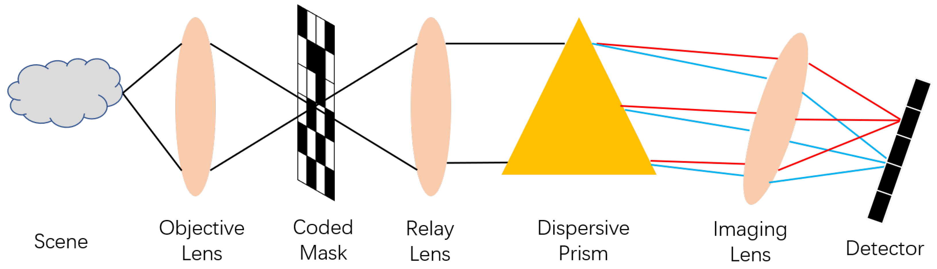
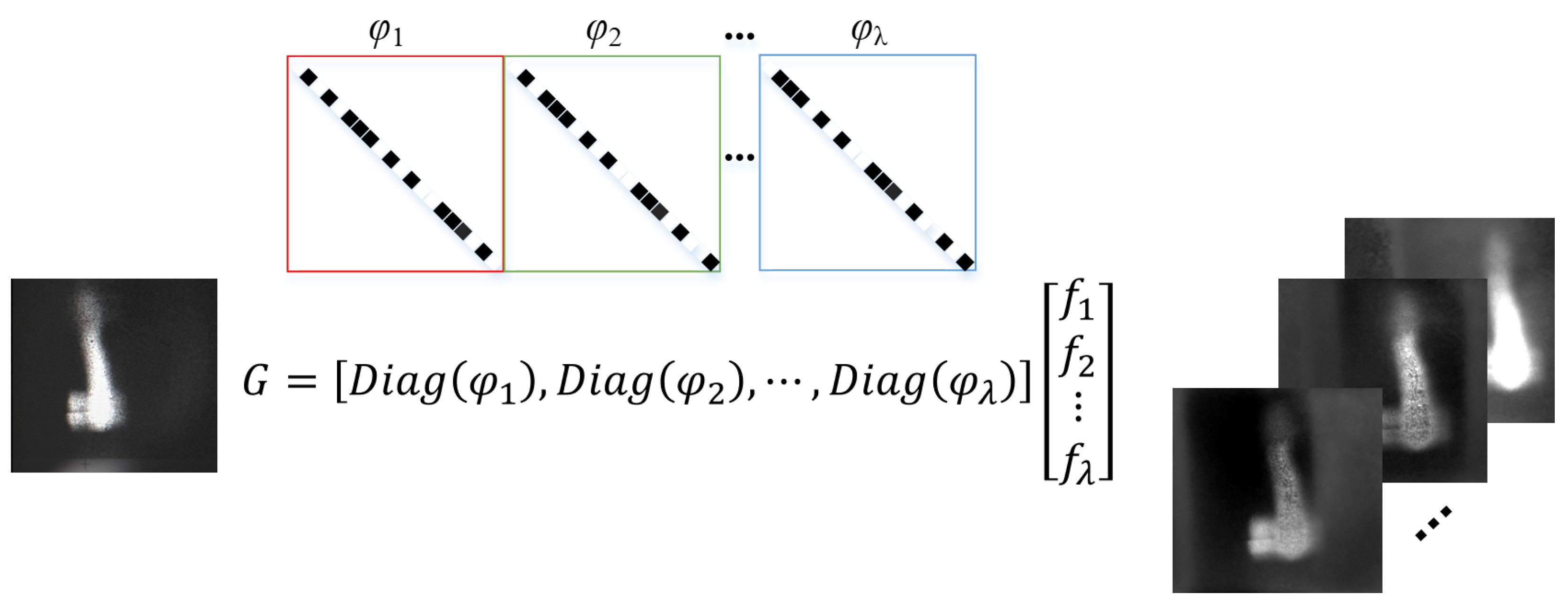
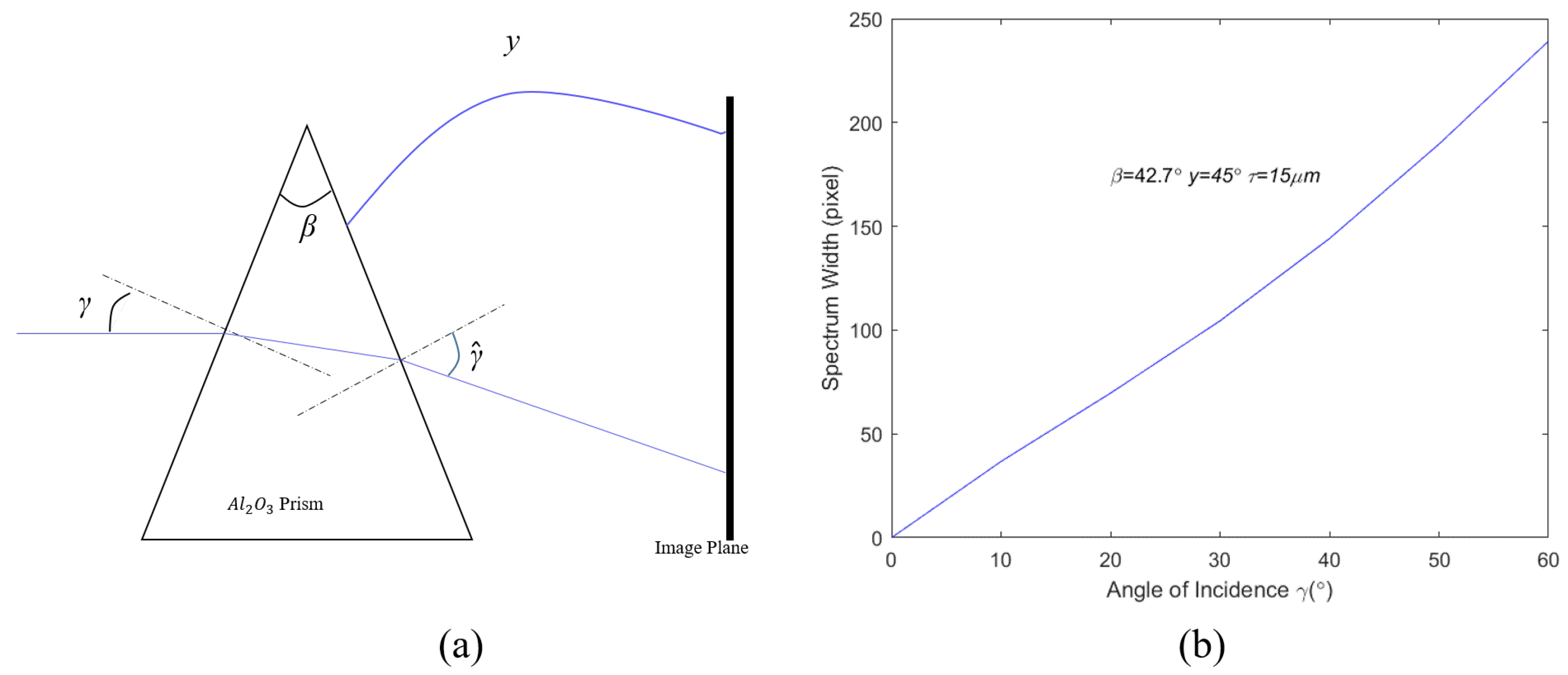
2. A Compressive Spectral Imaging Model

The basic idea of compressive spectral imaging is to encode a 3D spatio-spectral data cube to a 2D detector forming a snapshot 2D measurement, as shown in Figure 1. The spectral scene is spatially encoded by the coded mask. The prism spectrally disperses the encoded scene. At last, a detector captures the spatial-spectral encoding scene.
For the spectral data cube of the scene X R n x × n y × B , where n x , n y , and B denote the width, height, and the number of spectral bands, respectively, and is compressed by B coded masks A R n x × n y × B into the measurements Y R n x × n y . We can mathematically form this process as
Y = b = 1 B A b X b + M
where b denotes the b-th coded mask and the corresponding spectral image. M R n x × n y denotes the measurement noise. ⊙ denotes the element-wise product. By vectorizing y = v e c ( Y ) R n x n y , x = v e c ( X ) R n x n y B , and m = v e c ( M ) R n x n y , Equation (1) can be written in matrix-vector form as
y = A x + m
After obtaining the measurement y, the spectral images can be recovered from reconstruction algorithms.

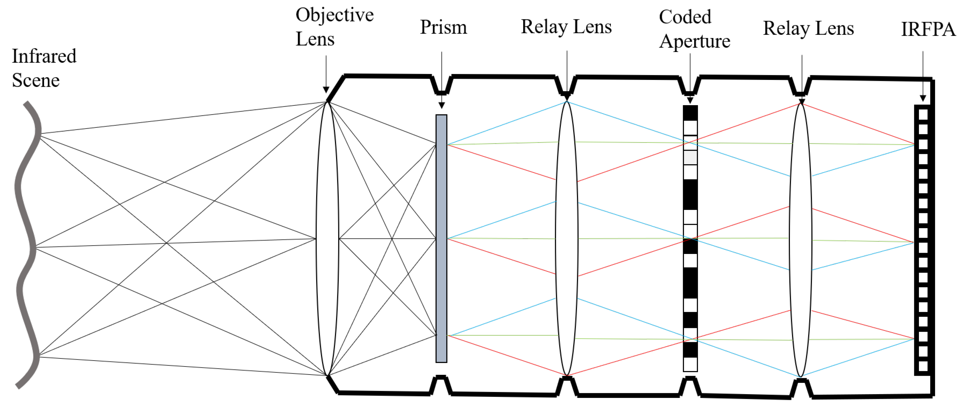
3. Optical Sensing and Reconstruction of the Proposed Architecture

A conceptual diagram of the MWIR-SCSI optical setup is presented in Figure 2. The scene’s infrared radiation is collected by an objective lens and then dispersed into the spectral plane by the prism. After a relay lens, a coded mask is mounted in front of the image plane, which allows the mask to modulate the spectral scene in both spatial and spectral dimensions. The encoded spectral image is focused onto the 2D IRFPA by the last relay lens. The captured 2D radiance field sampled by our system includes light multiplexed from the spatio-spectral encoded of the entire scene. The mathematical model of the sensing process is represented as follows:
The scene information of a 3D spectral clip in discrete form is denoted by Z i , j , λ , where 1 i W and 1 j H are the spatial coordinates, and 1 λ Ω denotes the spectral channels. Therefore, we can write the IRFPA measurement obtained during the entire interval as follows:
g ( i , j ) = λ = 1 Ω w ( λ ) O i , j σ ( λ ) z i , j σ ( λ ) , λ
where O ( i , j ) is the transfer function of the coded mask, w ( λ ) is the point spread function (PSF) achieved by the optical system, and σ ( λ ) denotes the dispersion function of the dispersion element. We can rewrite the formula of Equation (3), as follows:
G = Φ Z
where G R W H × 1 is a representation of g by vectorization, and Z = z 1 , z 2 , , z λ T R W H Ω × 1 denotes the vectorized representation of the original spectral images. Since the spectral images are dispersed to different positions on the coded aperture, the spectral images are encoded by different sensing matrices φ k , k = 1 , , λ . Thus, we let Φ R W H × W H Ω denote the sensing matrices of the coded spectral images, and it can be expressed as
Φ = [ D i a g ( φ 1 ) , D i a g ( φ 2 ) , , D i a g ( φ λ ) ]
where D i a g ( · ) is a diagonal matrix, and the vector φ k forms diagonal elements. The entire sensing process is depicted in Figure 3.
Thus, the spectral images reconstruction is formulated as a recovery problem of a fitting data term with an additional regularization term:
Z ˜ = arg min Z G Φ Z 2 2 + ρ K Z
where ρ denotes the Lagrange parameter that balances sparsity and the regularization term K ( Z ) during optimization. We further solve Equation (6) using the PnP algorithm with a deep infrared denoising prior, described in the next section.

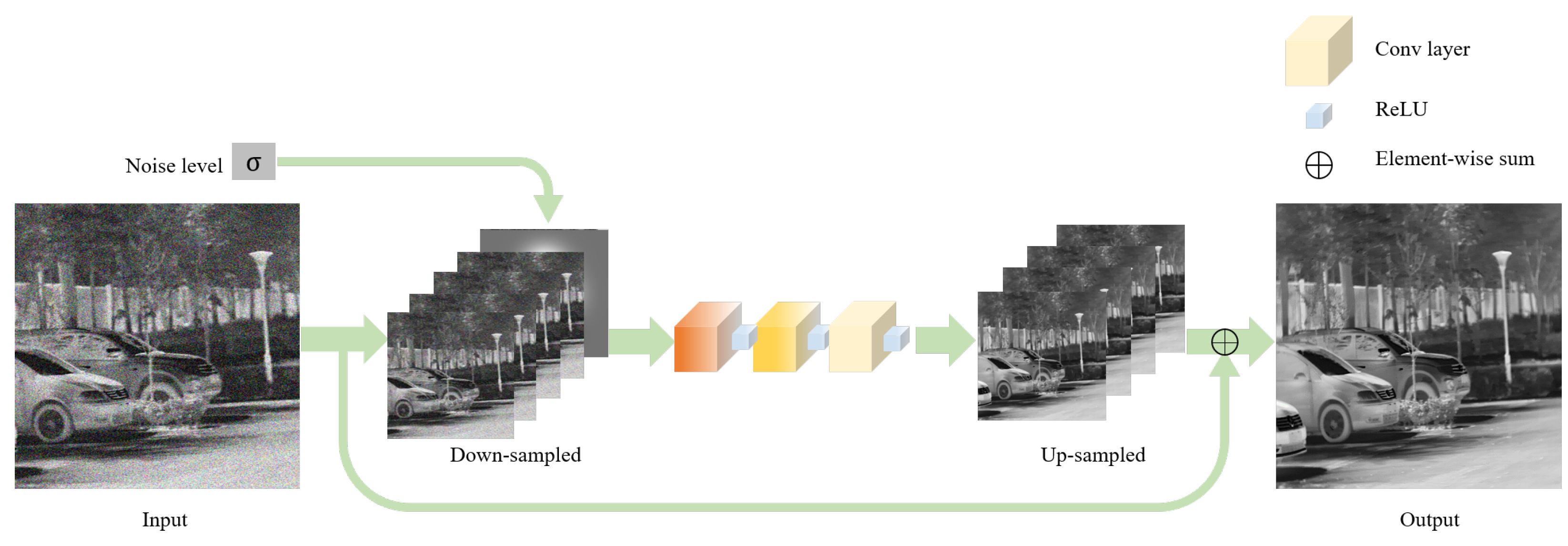
4. A Deep Infrared Denoising Prior for Hyperspectral Image Reconstruction

In the optimization-based methods, the GAP-TV algorithm has shown impressive performance in compressive sensing reconstruction [48]. The generalized alternating projection (GAP) framework applies a faster denoiser and total variation (TV), but the denoiser cannot achieve high-quality results. Recently, deep learning approaches have been used to resolve recovery problems of visible snapshot compressive imaging for rapid and raised effects [35,39,40,41,42,44,45,46]. However, these system-specific networks cannot be directly applied to our task due to the lack of infrared hyperspectral datasets for network training. From the idea of the recent advance of the PnP image restoration, it has demonstrated that a proper denoiser can act as the image prior for optimization-based algorithms to solve the recovery problem of Equation (6). To leverage the advantage of GAP, a deep infrared denoising network is designed as the spatio-spectral prior and integrated into GAP for reconstruction. The GAP solution to the recovery problem of Equation (6) can be represented as
Z ( t + 1 ) = v ( t ) + Φ T ( Φ Φ T ) 1 ( G Φ v ( t ) )
v ( k + 1 ) = D σ ( F ( t + 1 ) )
where ( t ) is the iteration number. The data is first projected on a linear manifold G = Φ F in Equation (7), and the projected data are then denoised during iteration in Equation (8).
A great challenge in our task of using deep denoisers as a prior is that the contrast of the infrared image is low, various noise levels from different IRFPAs appear in the captured infrared image, and the inconspicuous features of the infrared image are difficult to extract. Therefore, the denoiser should be robust to adapt to different noise levels. We designed a deep infrared denoising network, as shown in Figure 4, and employed it in the denoising step of Equation (8), which can be formulated as
D σ ( Z ( t + 1 ) ) = arg min v g ( v ) + 1 2 Z ( t + 1 ) v 2 2
where g ( v ) is the regularization term. Given the noisy infrared image v, the clean infrared image can be obtained by our deep infrared denoising network.
To adapt the character of the infrared image, the noisy infrared image is down-sampled into four sub-images by convolution, as shown in Figure 4, and we then concatenate an estimated noise level map with noise deviation σ of additive white Gaussian noise (AWGN) as an input of the network. A data cube of size W 2 × H 2 × ( 4 C + 1 ) is then transported into a CNN with 14 convolution blocks ( [ C o n v + R e L U ] × 14 ). The residual learning strategy is adopted for a faster convergence [49]. A convolutional kernel of size 3 × 3 and zero padding are employed to maintain the feature map size during convolution. To produce the denoised infrared image with its original image size W × H , the PixelShuffle operation [50,51] is applied to up-sample at the last step. Hereby, the denoised infrared image is obtained and then served for the next iteration. Our code is available at https://github.com/shuowenyang/GAP-DIDNet (accessed on 28 December 2022).

5. Simulation Results

5.1. Training Details of the Infrared Denoising Network

We used a cooled mid-wave infrared camera (TB-M640-CL) to obtain 100 infrared images of size 640 × 512 (see Figure 5). We then cropped images into patches with a size of 64 × 64 , and applied data augmentation methods (flip, rotation, and scale) to increase the number of training samples. A similar operation was performed on another 20 images for testing. We added AWGN with a noise level of σ [0, 75] to the original images to generate a noisy version. PyTorch [52] was used for the implementation, and ADAM [53] was chosen as the optimizer. The training epochs were set to 100 with a learning rate starting from 10 3 , which decayed 10 times every 50 training epochs.

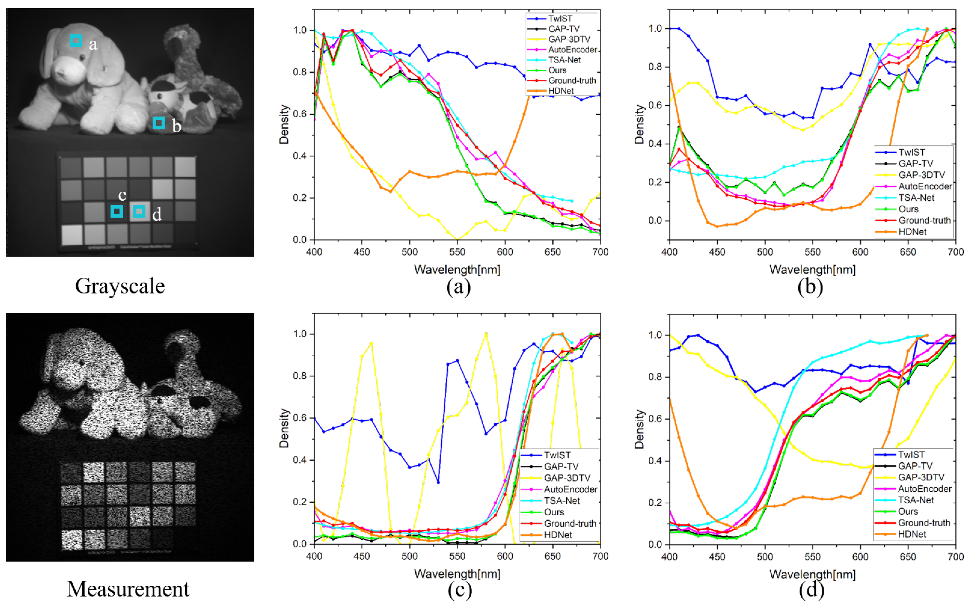
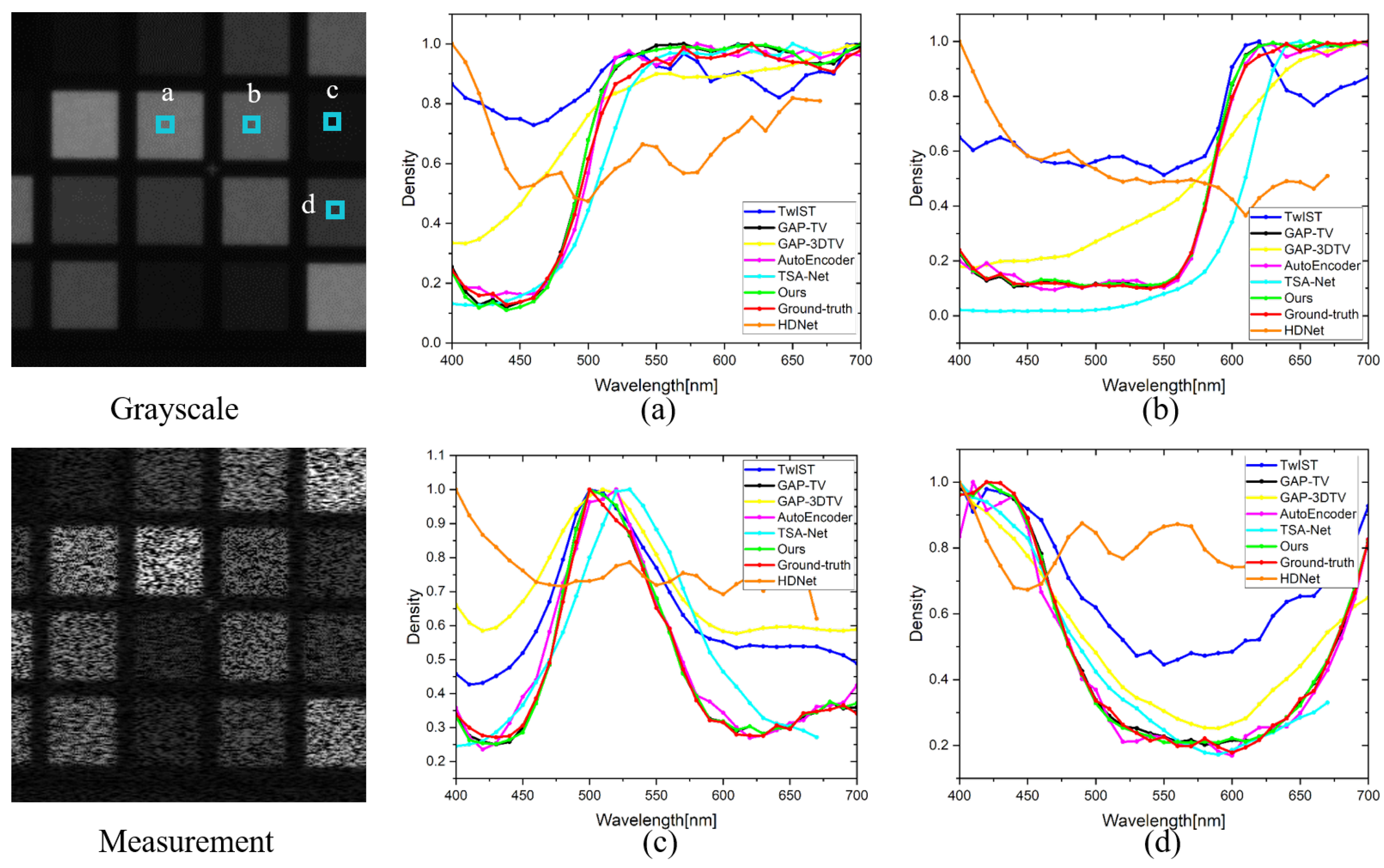
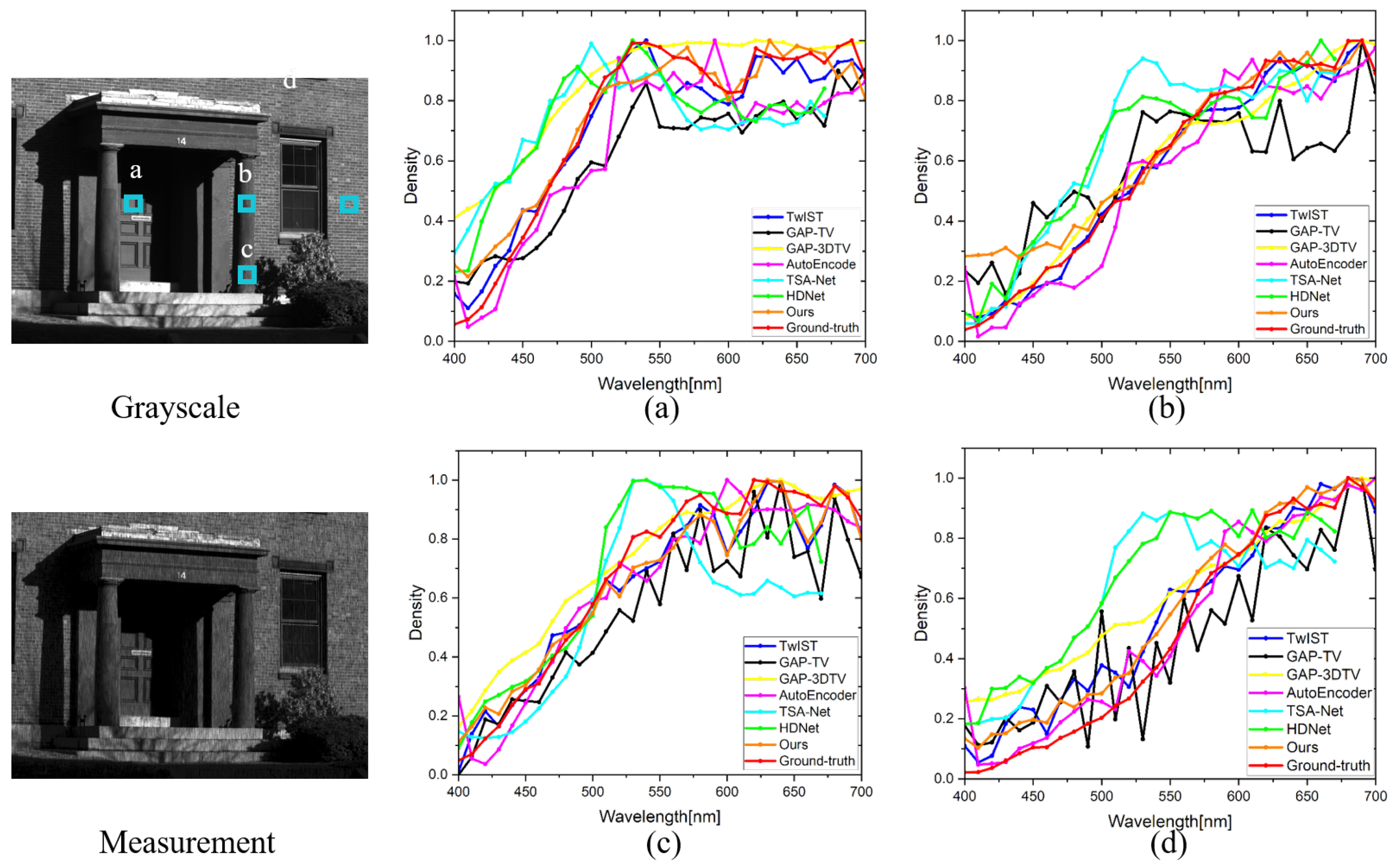
5.2. Algorithm Evaluation

We conducted simulation experiments to demonstrate the hardware principle and the proposed reconstruction algorithm. For the simulation data, we employed the publicly available datasets CAVE [54], KAIST [55], and Harvard [56] and transformed the images into grayscale images. We then generated measurements following our MWIR-SCSI framework using the shifting random binary mask. The proposed reconstruction algorithm competes with other popular methods, including TwIST [57], GAP-TV [48], GAP-3DTV [58], AutoEncoder [55], TSA-Net [59], and HDNet [60]. We assessed the performance of these competing methods by four metrics: peak signal-to-noise ratio (PSNR), structural similarity (SSIM) [61], the spectral angular mapper (SAM) [62], and running time.
The average PSNR, SSIM, and SAM on the entire CAVE and KAIST datasets constructed by the aforementioned algorithms are listed in Table 1. We can observe that the PSNR and SSIM values of the optimization-based GAP algorithms are much higher than the CNN-based TSA-Net. The table also shows that the AutoEncoder method is outstanding, as it can outperform the other methods. It achieved the best results in the SAM. The reason for this may be that this algorithm learns nonlinear spectral representations from real-world hyperspectral datasets. As a comparison, the proposed algorithm achieves a further promotion in PSNR and SSIM and ranks second in terms of SAM. It can be observed that the GAP algorithms can achieve considerable results compared with the ordinary reconstruction methods TwIST and TSA-Net. This indicates that the PnP framework can perform substantially well in spectral image reconstruction. However, the traditional denoisers (TV and 3DTV) are insufficient. In terms of the performance comparison of our proposed algorithm and the learning-based algorithms, our algorithm is excellent in PSNR and SSIM and ranks second in terms of the SAM because our algorithm plugs in a deep denoiser, exploiting the advantages of both optimization-based algorithms and learning-based algorithms.
Further, to evaluate the fidelity of reconstructed spectral images, we tried to calculate the accuracy, precision, recall, and F1-score for verification. Because the original and reconstructed spectral images are grayscale instead of binary, we normalized the values between 0 and 1, and we then set the values of the images greater than 0.5 to 1 to calculate these indexes, as shown in Table 2. The results show that the learning-based algorithms are capable of achieving a higher fidelity than the optimization-based ones. In particular, the proposed method produces the best results.
In terms of running time, the reconstruction of the CAVE data of spatial size 512 × 512 , the KAIST data of spatial size 256 × 256 , and the Harvard data of spatial size 1040 × 1392 is shown in Table 3 for each method. The codes of the optimization-based methods were written using MATLAB and run on a CPU. The deep-learning-based methods were written in Python and run on a GPU. With the increase in image size, the time consumption also increases, but for deep learning algorithms, parallel operation can effectively save time. It is observed that the GAP-based methods have a speed advantage, but the reconstruction results of these algorithms are far from optimum. The AutoEncoder method requires a high amount of training time to obtain the spectral prior. The time-consuming TSA-Net benefits from deep learning. Although our strategy requires iterative processing during the estimation, it demonstrates an acceptable amount of time consumption for the network test on the GPU by combining the pre-trained deep denoiser.
To visualize the experimental results, the spatial details and spectral accuracy of the reconstructed results by different algorithms on images from the CAVE, KAIST, and Harvard datasets are compared in Figure 6, Figure 7 and Figure 8, respectively. The reconstructed frames of TwIST are not clean. GAP-TV can provide visually decent results, whereas GAP-3DTV suffers from blurry details. Although AutoEncoder, TSA-Net, and HDNet, as CNN-based methods, can recover most spatial details, some areas have blurred edges and lost detail, especially using the TSA-Net algorithm. By contrast, our method benefits from both the GAP and the deep denoiser, and thus displays sharper edges and higher visual quality. Significantly, the drawback of learning-based methods is even more obvious in large-size images because they rely heavily on training data, and more training parameters are required. Optimization-based algorithms can fill this gap. Thus, the combination of learning-based and optimization-based methods, i.e., the proposed method, can maintain performance well. Furthermore, the reconstructed spectral curves of the four special regions were plotted to compare the spectral accuracy, shown in Figure 9, Figure 10 and Figure 11. The reconstructed spectral curves of the proposed method have a higher consistency with the ground-truth spectra. The spectral curves of TwIST and GAP-3DTV deviate from the ground truth the most.

6. Experiment Results

6.1. MWIR Snapshot Compressive Spectral Imager Design

To experimentally evaluate the effectiveness of the proposed architecture, a proof-of-concept MWIR-SCSI system was established, as shown in Figure 12. An objective lens (focal length: 127 mm; diameter: 50 mm) was used to optically form the scene’s infrared radiation on the prism (customized AL 2 O 3 ). The dispersed spectral scene was coded by a coded aperture, which is a lithographically patterned chrome-on-Ge mask. In our experiments, the mask we used was a Gaussian random pattern with the same resolution and pixel pitch as the IRFPA. Furthermore, each mask pixel was represented by a 1 × 1 window of IRFPA pixel subsets, so the maximum modulation resolution was 640 × 512. To flexibly adjust the mask-IRFPA distance, another relay lens (focal length 125 mm, f) was used to transfer the spatio-spectral modulation of the scene onto the IRFPA with a resolution 640 × 512 and a pixel size of 15 μ m.

6.2. Spatial, Temporal, and Spectral Resolution

In our MWIR-SCSI system, the spatial resolution and temporal resolution are determined by the IRFPA and its frame rate, respectively. Therefore, our MWIR-SCSI system can capture a maximum spatial resolution of 640 × 512 and a maximum temporal resolution of 50 fps. Both the dispersed spectrum width on the IRFPA plane and the IRFPA pixel size determine the spectral resolution. The calculation process of spectral resolution is as follows:
Figure 13a shows the optical path in the AL 2 O 3 prism. The outgoing ray angle γ ^ is represented in Equation (10):
γ ^ ( c ) = a r c s i n β a r c s i n s i n γ n ( c )
where n ( · ) denotes the refractive index of the AL 2 O 3 prism, with incident light wavelength c, β indicates the angle of the AL 2 O 3 prism, γ denotes the angle of incidence, and y represents the position between the image plane and the prism. The spectral resolution can be calculated by Equation (11):
R s p e = ψ τ = f t a n γ ^ ( c e ) y t a n γ ^ ( c s ) y τ
where ψ denotes the dispersed spectrum width, τ denotes the IRFPA array size, and f denotes the imaging focal length. c e and c s are the maximum and minimum wavelengths in the angle of refraction of the outgoing rays, respectively. Figure 13b shows the spectral resolution R s p e curve from 3.7 μ m to 4.8 μ m in MWIR-SCSI.

6.3. System Calibration

Equation (6) indicates the features of this coding pattern Φ have a great influence on the fidelity of the estimated spectral images. In most simulation experiments, the coding pattern is regarded as a binary pattern, whereas the infrared radiation does not entirely penetrate the coded mask or reflect completely in the experiment. In addition, the response of the IRFPA to infrared radiation is inconsistent, which is also the case with other infrared optical components. As a result, the coding pattern used in the reconstruction cannot be regarded as a binary pattern but as a grayscale pattern.
Therefore, system calibration is necessary to correct this theoretical error to reconstruct accurate spectral images. The response of our system or the PSF to each pixel source of the different spectral scenes can be obtained to achieve this process. We simplify this operation by obtaining the experimental coded matrix Φ . Specifically, we uniformly illuminate the MWIR-SCSI system with each monochromatic wavelength of light in 10 nm increments from 3.7 μ m to 4.8 μ m and capture 111 monochrome images of the coded mask.
Some of the results are shown in Figure 14. We can see that from 3.7 μ m to 4.8 μ m, the coded mask shift with different displacements, as well as the dispersion at the shorter end of the spectrum, is less than that at the longer end, which demonstrates the non-linear spectral response of the entire system, covering the non-linearity of the prism dispersion. All of the mask images of 111 spectral channels contain the information that the reconstruction algorithm attempts to recover. The wavelength curve according to the position of the cross on the template images is shown in Figure 15. Essentially, this nonlinear curve discretely represents the dispersion coefficient of the proposed MWIR-SCSI system.
Similar to the process above, we set the values of the captured coded mask images greater than 0.5 to 1. We generated a 0–1 Gaussian random matrix to produce the coded aperture (Figure 12). Thus, the accuracy, precision, recall, and F1-score can be calculated, as shown in Table 4. These values are not very high, which indicates the theoretical and practical gap caused by the nonlinear response of the system.

6.4. Results and Discussion

To demonstrate the spectral imaging capability, our MWIR-SCSI system recorded measurement images at mid-wave infrared wavelengths from the sample combustion process (candle flame) at live video frame rates, as shown in Figure 16a. The partial results of 32 wavelength channels between 3.7 and 4.8 μ m using the proposed reconstruction method are shown in Figure 17. In order to demonstrate the hyperspectral image acquisition capability of the proposed MWIR-SCSI system for dynamic targets, we measured another candle flame in motion, as shown in Figure 16b. Similarly, the restored results by the proposed reconstruction method are shown in Figure 18. Our system and algorithm were able to obtain the candle flame details well and distinguish significant spectral differences. The longer the wavelength, the darker the outer flame, and the brighter the inner flame. This observation can be explained by the temperature variation—the temperature of the outer flame is higher than that of the inner flame, so more radiation energy is distributed over shorter wavelengths, while the radiation energy of the inner flame is higher over longer wavelengths. The spectral curves selected from the outer and inner flame are presented in Figure 16c. The strong CO 2 absorption in the gap at 4.3 μ m is also clearly presented in the figure. This provides a reliable way to identify the chemical composition of different flames by imaging at different wavelengths.
In mid-wave infrared, we have reported another low-cost computational spectral imaging system [34], which leverages the DMD and spectrometer to collect measurement signals through multiple encoding. This strategy only conducts spatial coding, whereas the proposed MWIR-SCSI system simultaneously performs spatial and spectral coding. Table 5 lists the significant differences between these devices. The MWIR-SCSI system makes it possible to achieve fast acquisition through single encoding. However, the main limitation of the MWIR-SCSI system is that traditional optimization algorithms require high amounts of time for reconstruction. Fortunately, the future development of deep learning methods can effectively address this problem.

7. Conclusions

In this work, we present a novel mid-wave infrared snapshot compressive spectral imager based on a prism and a coded aperture to produce spatio-spectral coded to the benefit of reconstruction. In addition, as an important step in the infrared imaging system, convenient and practical calibration methods are implemented in our system. We acquire 111 real coded masks in which the displacement reflects the non-linear spectral response of the entire system. To address inconsistencies in infrared image noise levels and missing datasets, the image reconstruction problem in our system is formulated as an inverse problem with the GAP plug-in deep infrared denoising network, ensuring smooth reconstructed images in spatial and spectral dimensions. Compared to traditional scanning architectures, the proposed MWIR-SCSI performs well in dynamic scenes because objects can be sparsely sampled at live video frame rates. Extensive results on a simulation dataset and real infrared scenarios obtained by our system have demonstrated the performance of both the proposed system and the method.

Author Contributions

S.Y. (Shuowen Yang) designed the system, made the experiments, and wrote the manuscript; H.Q. reviewed and edited; X.Y. assisted in the preparation work; S.Y. (Shuai Yuan) discussed the results; Q.Z. provided some comments. All authors contributed to the improvement of the manuscript’s presentation. All authors have read and agreed to the published version of the manuscript.

Funding

This work was supported in part by the National Natural Science Foundation of China (No.61901330), the Science and Technology Project of Xi’an (No.21JBGSZ-QCY9-0004), the National Key R & D Program of China (No.2021YFF0308100), and the China Postdoctoral Science Foundation (No.2019M653566).

Data Availability Statement

The datasets presented in this study are available in [54,55,56].

Acknowledgments

The authors would like to express their gratitude to the anonymous reviewers and editors who worked tirelessly to improve our manuscript.

Conflicts of Interest

The authors declare that they have no conflict of interest.

References

  1. Sidran, M. Broadband reflectance and emissivity of specular and rough water surfaces. Appl. Opt. 1981, 20, 3176–3183. [Google Scholar] [CrossRef] [PubMed]
  2. Diener, R.; Tepper, J.; Labadie, L.; Pertsch, T.; Nolte, S.; Minardi, S. Towards 3D-photonic, multi-telescope beam combiners for mid-infrared astrointerferometry. Opt. Express 2017, 25, 19262–19274. [Google Scholar] [CrossRef]
  3. Amrania, H.; Antonacci, G.; Chan, C.H.; Drummond, L.; Otto, W.R.; Wright, N.A.; Phillips, C. Digistain: A digital staining instrument for histopathology. Opt. Express 2012, 20, 7290–7299. [Google Scholar] [CrossRef] [PubMed]
  4. Junaid, S.; Kumar, S.C.; Mathez, M.; Hermes, M.; Stone, N.; Shepherd, N.; Ebrahim-Zadeh, M.; Tidemand-Lichtenberg, P.; Pedersen, C. Video-rate, mid-infrared hyperspectral upconversion imaging. Optica 2019, 6, 702–708. [Google Scholar] [CrossRef] [Green Version]
  5. Elsner, A.E.; Weber, A.; Cheney, M.C.; VanNasdale, D.A.; Miura, M. Imaging polarimetry in patients with neovascular age-related macular degeneration. JOSA A 2007, 24, 1468–1480. [Google Scholar] [CrossRef] [Green Version]
  6. Dombrowski, M.S.; Willson, P.D. Video rate visible to LWIR hyperspectral image generation and exploitation. In Proceedings of the Internal Standardization and Calibration Architectures for Chemical Sensors, Boston, MA, USA, 20–22 September 1999; International Society for Optics and Photonics: Bellingham, WA, USA, 1999; Volume 3856, pp. 24–33. [Google Scholar]
  7. Schreer, O.; Zettner, J.; Spellenberg, B.; Schmidt, U.; Danner, A.; Peppermueller, C.; Saenz, M.L.; Hierl, T. Multispectral high-speed midwave infrared imaging system. In Proceedings of the Infrared Technology and Applications XXX, Orlando, FL, USA, 12–16 April 2004; International Society for Optics and Photonics: Bellingham, WA, USA, 2004; Volume 5406, pp. 249–257. [Google Scholar]
  8. Chamberland, M.; Farley, V.; Tremblay, P.; Legault, J.F. Performance model of imaging FTS as a standoff chemical agent detection tool. In Chemical and Biological Standoff Detection; International Society for Optics and Photonics: Bellingham, WA, USA, 2004; Volume 5268, pp. 240–251. [Google Scholar]
  9. Amenabar, I.; Poly, S.; Goikoetxea, M.; Nuansing, W.; Lasch, P.; Hillenbrand, R. Hyperspectral infrared nanoimaging of organic samples based on Fourier transform infrared nanospectroscopy. Nat. Commun. 2017, 8, 14402. [Google Scholar] [CrossRef] [Green Version]
  10. Gupta, N.; Dahmani, R.; Bennett, K.; Simizu, S.; Suhre, D.R.; Singh, N. Progress in AOTF hyperspectral imagers. In Proceedings of the Automated Geo-Spatial Image and Data Exploitation, Orlando, FL, USA, 24 April 2000; International Society for Optics and Photonics: Bellingham, WA, USA, 2000; Volume 4054, pp. 30–38. [Google Scholar]
  11. Zhao, H.; Ji, Z.; Jia, G.; Zhang, Y.; Li, Y.; Wang, D. MWIR thermal imaging spectrometer based on the acousto-optic tunable filter. Appl. Opt. 2017, 56, 7269–7276. [Google Scholar] [CrossRef]
  12. Dam, J.S.; Tidemand-Lichtenberg, P.; Pedersen, C. Room-temperature mid-infrared single-photon spectral imaging. Nat. Photonics 2012, 6, 788–793. [Google Scholar] [CrossRef] [Green Version]
  13. Junaid, S.; Tomko, J.; Semtsiv, M.P.; Kischkat, J.; Masselink, W.T.; Pedersen, C.; Tidemand-Lichtenberg, P. Mid-infrared upconversion based hyperspectral imaging. Opt. Express 2018, 26, 2203–2211. [Google Scholar] [CrossRef] [Green Version]
  14. Donoho, D.L. Compressed sensing. IEEE Trans. Inf. Theory 2006, 52, 1289–1306. [Google Scholar] [CrossRef]
  15. Gehm, M.E.; John, R.; Brady, D.J.; Willett, R.M.; Schulz, T.J. Single-shot compressive spectral imaging with a dual-disperser architecture. Opt. Express 2007, 15, 14013–14027. [Google Scholar] [CrossRef] [PubMed] [Green Version]
  16. Wagadarikar, A.; John, R.; Willett, R.; Brady, D. Single disperser design for coded aperture snapshot spectral imaging. Appl. Opt. 2008, 47, B44–B51. [Google Scholar] [CrossRef] [PubMed] [Green Version]
  17. Kittle, D.; Choi, K.; Wagadarikar, A.; Brady, D.J. Multiframe image estimation for coded aperture snapshot spectral imagers. Appl. Opt. 2010, 49, 6824–6833. [Google Scholar] [CrossRef]
  18. Arguello, H.; Arce, G.R. Colored coded aperture design by concentration of measure in compressive spectral imaging. IEEE Trans. Image Process. 2014, 23, 1896–1908. [Google Scholar] [CrossRef] [PubMed]
  19. Lin, X.; Liu, Y.; Wu, J.; Dai, Q. Spatial-spectral encoded compressive hyperspectral imaging. ACM Trans. Graph. (TOG) 2014, 33, 1–11. [Google Scholar] [CrossRef]
  20. Yuan, X.; Tsai, T.H.; Zhu, R.; Llull, P.; Brady, D.; Carin, L. Compressive hyperspectral imaging with side information. IEEE J. Sel. Top. Signal Process. 2015, 9, 964–976. [Google Scholar] [CrossRef] [Green Version]
  21. Wang, L.; Xiong, Z.; Gao, D.; Shi, G.; Wu, F. Dual-camera design for coded aperture snapshot spectral imaging. Appl. Opt. 2015, 54, 848–858. [Google Scholar] [CrossRef] [Green Version]
  22. Liu, X.; Yu, Z.; Zheng, S.; Li, Y.; Tao, X.; Wu, F.; Xie, Q.; Sun, Y.; Wang, C.; Zheng, Z. Residual image recovery method based on the dual-camera design of a compressive hyperspectral imaging system. Opt. Express 2022, 30, 20100–20116. [Google Scholar] [CrossRef]
  23. Xie, H.; Zhao, Z.; Han, J.; Zhang, Y.; Bai, L.; Lu, J. Dual camera snapshot hyperspectral imaging system via physics-informed learning. Opt. Lasers Eng. 2022, 154, 107023. [Google Scholar] [CrossRef]
  24. Li, X.; Greenberg, J.A.; Gehm, M.E. Single-shot multispectral imaging through a thin scatterer. Optica 2019, 6, 864–871. [Google Scholar] [CrossRef]
  25. Saragadam, V.; DeZeeuw, M.; Baraniuk, R.G.; Veeraraghavan, A.; Sankaranarayanan, A.C. SASSI—Super-pixelated adaptive spatio-spectral imaging. IEEE Trans. Pattern Anal. Mach. Intell. 2021, 43, 2233–2244. [Google Scholar] [CrossRef] [PubMed]
  26. Arguello, H.; Pinilla, S.; Peng, Y.; Ikoma, H.; Bacca, J.; Wetzstein, G. Shift-variant color-coded diffractive spectral imaging system. Optica 2021, 8, 1424–1434. [Google Scholar] [CrossRef]
  27. Mahalanobis, A.; Shilling, R.; Murphy, R.; Muise, R. Recent results of medium wave infrared compressive sensing. Appl. Opt. 2014, 53, 8060–8070. [Google Scholar] [CrossRef] [PubMed]
  28. Zhang, L.; Ke, J.; Chi, S.; Hao, X.; Yang, T.; Cheng, D. High-resolution fast mid-wave infrared compressive imaging. Opt. Lett. 2021, 46, 2469–2472. [Google Scholar] [CrossRef]
  29. Wu, Z.; Wang, X. Focal plane array-based compressive imaging in medium wave infrared: Modeling, implementation, and challenges. Appl. Opt. 2019, 58, 8433–8441. [Google Scholar] [CrossRef] [PubMed]
  30. Wu, Z.; Wang, X. Non-uniformity correction for medium wave infrared focal plane array-based compressive imaging. Opt. Express 2020, 28, 8541–8559. [Google Scholar] [CrossRef] [PubMed]
  31. Russell, T.A.; McMackin, L.; Bridge, B.; Baraniuk, R. Compressive hyperspectral sensor for LWIR gas detection. In Compressive Sensing; International Society for Optics and Photonics: Bellingham, WA, USA, 2012; Volume 8365, p. 83650C. [Google Scholar]
  32. Dupuis, J.R.; Kirby, M.; Cosofret, B.R. Longwave infrared compressive hyperspectral imager. In Proceedings of the Next-Generation Spectroscopic Technologies VIII; International Society for Optics and Photonics: Bellingham, WA, USA, 2015; Volume 9482, p. 94820Z. [Google Scholar]
  33. Gattinger, P.; Kilgus, J.; Zorin, I.; Langer, G.; Nikzad-Langerodi, R.; Rankl, C.; Gröschl, M.; Brandstetter, M. Broadband near-infrared hyperspectral single pixel imaging for chemical characterization. Opt. Express 2019, 27, 12666–12672. [Google Scholar] [CrossRef]
  34. Yang, S.; Yan, X.; Qin, H.; Zeng, Q.; Liang, Y.; Arguello, H.; Yuan, X. Mid-Infrared Compressive Hyperspectral Imaging. Remote Sens. 2021, 13, 741. [Google Scholar] [CrossRef]
  35. Yuan, X.; Brady, D.J.; Katsaggelos, A.K. Snapshot compressive imaging: Theory, algorithms, and applications. IEEE Signal Process. Mag. 2021, 38, 65–88. [Google Scholar] [CrossRef]
  36. Sullenberger, R.; Milstein, A.; Rachlin, Y.; Kaushik, S.; Wynn, C. Computational reconfigurable imaging spectrometer. Opt. Express 2017, 25, 31960–31969. [Google Scholar] [CrossRef]
  37. Xiang, F.; Huang, Y.; Gu, X.; Liang, P.; Zhang, J. A restoration method of infrared image based on compressive sampling. In Proceedings of the 2016 8th International Conference on Intelligent Human-Machine Systems and Cybernetics (IHMSC), Hangzhou, China, 27–28 August 2016; Volume 1, pp. 493–496. [Google Scholar]
  38. Emerson, T.H.; Olson, C.C.; Lutz, A. Image Recovery in the Infrared Domain via Path-Augmented Compressive Sampling Matching Pursuit. In Proceedings of the IEEE/CVF Conference on Computer Vision and Pattern Recognition Workshops, Long Beach, CA, USA, 16–17 June 2019. [Google Scholar]
  39. Meng, Z.; Yu, Z.; Xu, K.; Yuan, X. Self-supervised neural networks for spectral snapshot compressive imaging. In Proceedings of the IEEE/CVF International Conference on Computer Vision, Nashville, TN, USA, 20–25 June 2021; pp. 2622–2631. [Google Scholar]
  40. Meng, Z.; Yuan, X. Perception inspired deep neural networks for spectral snapshot compressive imaging. In Proceedings of the 2021 IEEE International Conference on Image Processing (ICIP), Anchorage, AK, USA, 19–22 September 2021; pp. 2813–2817. [Google Scholar]
  41. Huang, T.; Dong, W.; Yuan, X.; Wu, J.; Shi, G. Deep gaussian scale mixture prior for spectral compressive imaging. In Proceedings of the IEEE/CVF Conference on Computer Vision and Pattern Recognition, Nashville, TN, USA, 20–25 June 2021; pp. 16216–16225. [Google Scholar]
  42. Sun, Y.; Yang, Y.; Liu, Q.; Kankanhalli, M. Unsupervised Spatial–Spectral Network Learning for Hyperspectral Compressive Snapshot Reconstruction. IEEE Trans. Geosci. Remote Sens. 2021, 60, 1–14. [Google Scholar] [CrossRef]
  43. Yang, S.; Qin, H.; Yan, X.; Yuan, S.; Yang, T. Deep spatial-spectral prior with an adaptive dual attention network for single-pixel hyperspectral reconstruction. Opt. Express 2022, 30, 29621–29638. [Google Scholar] [CrossRef] [PubMed]
  44. Wang, L.; Wu, Z.; Zhong, Y.; Yuan, X. Snapshot spectral compressive imaging reconstruction using convolution and contextual Transformer. Photonics Res. 2022, 10, 1848–1858. [Google Scholar] [CrossRef]
  45. Cai, Y.; Lin, J.; Hu, X.; Wang, H.; Yuan, X.; Zhang, Y.; Timofte, R.; Van Gool, L. Mask-guided spectral-wise transformer for efficient hyperspectral image reconstruction. In Proceedings of the IEEE/CVF Conference on Computer Vision and Pattern Recognition, New Orleans, LA, USA, 19–20 June 2022; pp. 17502–17511. [Google Scholar]
  46. Zhang, X.; Zhang, Y.; Xiong, R.; Sun, Q.; Zhang, J. HerosNet: Hyperspectral Explicable Reconstruction and Optimal Sampling Deep Network for Snapshot Compressive Imaging. In Proceedings of the IEEE/CVF Conference on Computer Vision and Pattern Recognition, New Orleans, LA, USA, 19–20 June 2022; pp. 17532–17541. [Google Scholar]
  47. Zhang, K.; Li, Y.; Zuo, W.; Zhang, L.; Van Gool, L.; Timofte, R. Plug-and-play image restoration with deep denoiser prior. IEEE Trans. Pattern Anal. Mach. Intell. 2021, 44, 6360–6376. [Google Scholar] [CrossRef] [PubMed]
  48. Yuan, X. Generalized alternating projection based total variation minimization for compressive sensing. In Proceedings of the 2016 IEEE International Conference on Image Processing (ICIP), Phoenix, AZ, USA, 25–28 September 2016; pp. 2539–2543. [Google Scholar]
  49. He, K.; Zhang, X.; Ren, S.; Sun, J. Deep residual learning for image recognition. In Proceedings of the IEEE Conference on Computer Vision and Pattern Recognition, Las Vegas, NV, USA, 26 June–1 July 2016; pp. 770–778. [Google Scholar]
  50. Shi, W.; Caballero, J.; Huszár, F.; Totz, J.; Aitken, A.P.; Bishop, R.; Rueckert, D.; Wang, Z. Real-time single image and video super-resolution using an efficient sub-pixel convolutional neural network. In Proceedings of the IEEE Conference on Computer Vision and Pattern Recognition, Las Vegas, NV, USA, 26 June–1 July 2016; pp. 1874–1883. [Google Scholar]
  51. Zhang, K.; Zuo, W.; Zhang, L. FFDNet: Toward a fast and flexible solution for CNN-based image denoising. IEEE Trans. Image Process. 2018, 27, 4608–4622. [Google Scholar] [CrossRef] [Green Version]
  52. Paszke, A.; Gross, S.; Massa, F.; Lerer, A.; Bradbury, J.; Chanan, G.; Killeen, T.; Lin, Z.; Gimelshein, N.; Antiga, L.; et al. Pytorch: An imperative style, high-performance deep learning library. In Proceedings of the 33rd Conference on Neural Information Processing System, Vancouver, BC, Canada, 8–14 December 2019; Volume 32. [Google Scholar]
  53. Kingma, D.P.; Ba, J. Adam: A method for stochastic optimization. arXiv 2014, arXiv:1412.6980. [Google Scholar]
  54. Yasuma, F.; Mitsunaga, T.; Iso, D.; Nayar, S.K. Generalized assorted pixel camera: Postcapture control of resolution, dynamic range, and spectrum. IEEE Trans. Image Process. 2010, 19, 2241–2253. [Google Scholar] [CrossRef] [Green Version]
  55. Choi, I.; Jeon, D.S.; Nam, G.; Gutierrez, D.; Kim, M.H. High-Quality Hyperspectral Reconstruction Using a Spectral Prior. ACM Trans. Graph. 2017, 36, 218. [Google Scholar] [CrossRef] [Green Version]
  56. Chakrabarti, A.; Zickler, T. Statistics of real-world hyperspectral images. In Proceedings of the CVPR 2011, Colorado Springs, CO, USA, 20–25 June 2011; pp. 193–200. [Google Scholar]
  57. Bioucas-Dias, J.M.; Figueiredo, M.A. A new TwIST: Two-step iterative shrinkage/thresholding algorithms for image restoration. IEEE Trans. Image Process. 2007, 16, 2992–3004. [Google Scholar] [CrossRef] [Green Version]
  58. Qiu, H.; Wang, Y.; Meng, D. Effective snapshot compressive-spectral imaging via deep denoising and total variation priors. In Proceedings of the IEEE/CVF Conference on Computer Vision and Pattern Recognition, Nashville, TN, USA, 20–25 June 2021; pp. 9127–9136. [Google Scholar]
  59. Meng, Z.; Ma, J.; Yuan, X. End-to-end low cost compressive spectral imaging with spatial-spectral self-attention. In Proceedings of the European Conference on Computer Vision, Glasgow, UK, 23–28 August 2020; Springer: Berlin/Heidelberg, Germany, 2020; pp. 187–204. [Google Scholar]
  60. Hu, X.; Cai, Y.; Lin, J.; Wang, H.; Yuan, X.; Zhang, Y.; Timofte, R.; Van Gool, L. Hdnet: High-resolution dual-domain learning for spectral compressive imaging. In Proceedings of the IEEE/CVF Conference on Computer Vision and Pattern Recognition, New Orleans, LA, USA, 19–20 June 2022; pp. 17542–17551. [Google Scholar]
  61. Wang, Z.; Bovik, A.C.; Sheikh, H.R.; Simoncelli, E.P. Image quality assessment: From error visibility to structural similarity. IEEE Trans. Image Process. 2004, 13, 600–612. [Google Scholar] [CrossRef] [Green Version]
  62. Kruse, F.A.; Lefkoff, A.; Boardman, J.; Heidebrecht, K.; Shapiro, A.; Barloon, P.; Goetz, A. The spectral image processing system (SIPS)—Interactive visualization and analysis of imaging spectrometer data. Remote Sens. Environ. 1993, 44, 145–163. [Google Scholar] [CrossRef]
Figure 1. Sensing process of compressive spectral imaging.
Remotesensing 15 00280 g001
Figure 2. Illustration of the MWIR-SCSI sampling scheme.
Remotesensing 15 00280 g002
Figure 3. Sensing model of the proposed MWIR-SCSI. The left side shows the measurement (coded image), the top side shows the coded mask, and the right side shows the spectral images.
Remotesensing 15 00280 g003
Figure 4. Network structure of the proposed deep infrared denoising prior.
Remotesensing 15 00280 g004
Figure 5. Representative infrared images captured by the cooled mid-wave infrared camera (TB-M640-CL). The features of most images are not clear.
Remotesensing 15 00280 g005
Figure 6. Reconstructed spectral images of s t u f f e d t o y s with a size of 512 × 512 from the CAVE dataset. We show the reconstructed result of four bands (wavelength: 420, 500, 600, and 700 nm) by different algorithms.
Remotesensing 15 00280 g006
Figure 7. Reconstructed spectral images with a size of 256 × 256 from the KAIST dataset. We show the reconstructed results of four bands (wavelength: 420, 500, 600, and 700 nm) by different algorithms.
Remotesensing 15 00280 g007
Figure 8. Reconstructed spectral images with a size of 1040 × 1392 from the Harvard dataset. We show the reconstructed results of four bands (wavelength: 420, 500, 600, and 700 nm) by different algorithms.
Remotesensing 15 00280 g008
Figure 9. Grayscale image and corresponding compressive measurement by the spatio-spectral encoding of s t u f f e d t o y s from the CAVE dataset. The right two columns display the reconstructed spectral curves on special regions to compare the spectral accuracy. (a) The spectral curves at point a; (b) The spectral curves at point b; (c) The spectral curves at point c; (d) The spectral curves at point d.
Remotesensing 15 00280 g009
Figure 10. Grayscale image and corresponding compressive measurement by the spatio-spectral encoding from the KAIST dataset. The right two columns display the reconstructed spectral curves on special regions to compare the spectral accuracy. (a) The spectral curves at point a; (b) The spectral curves at point b; (c) The spectral curves at point c; (d) The spectral curves at point d.
Remotesensing 15 00280 g010
Figure 11. Grayscale image and corresponding compressive measurement by the spatio-spectral encoding from the Harvard dataset. The right two columns display the reconstructed spectral curves on special regions to compare the spectral accuracy. (a) The spectral curves at point a; (b) The spectral curves at point b; (c) The spectral curves at point c; (d) The spectral curves at point d.
Remotesensing 15 00280 g011
Figure 12. Experiment setup implemented in the laboratory.
Remotesensing 15 00280 g012
Figure 13. (a) Optical path in the AL 2 O 3 prism: β denotes the prism angle, γ denotes the incident angle, y denotes the angle of the prism’s surface with the imaging plane, and γ ^ denotes the outgoing ray angle. (b) Spectrum width in our proposed system with a different incident angle γ .
Remotesensing 15 00280 g013
Figure 14. The MWIR-SCSI system response to uniform illumination of the coded mask at 11 different monochromatic wavelengths.
Remotesensing 15 00280 g014
Figure 15. The blue dots denote the position of the cross at the top of the coded mask as a function of wavelength and show nonlinear dispersion through a prism.
Remotesensing 15 00280 g015
Figure 16. (a) Single frame measurement image of candle flame captured by our MWIR-SCSI; (b) another frame measurement image of candle flames captured by our MWIR-SCSI; (c) the spectral curves selected from the outer flame and inner flame, respectively.
Remotesensing 15 00280 g016
Figure 17. Reconstructed spectral images by our reconstruction method.
Remotesensing 15 00280 g017
Figure 18. Reconstructed spectral images by our reconstruction method.
Remotesensing 15 00280 g018
Table 1. Average PSNR and SSIM comparison of competing methods on the CAVE, KAIST, and Harvard datasets.
DatasetsIndexTwISTGAP-TVGAP-3DTVAutoEncoderTSA-NetHDNetOurs
CAVEPSNR23.7429.0729.1532.4626.1032.1833.03
SSIM0.85230.92190.88660.92350.81050.90240.9257
SAM16.403311.596914.73214.799115.874313.748311.1254
KAISTPSNR23.7835.6028.2532.6423.6533.5835.73
SSIM0.86230.94680.87080.94750.79100.94280.9494
SAM15.22226.038912.34033.066314.25717.98345.8549
HarvardPSNR22.8430.2328.1931.8423.2832.0232.73
SSIM0.83460.92040.87390.92140.80430.93120.9345
SAM16.346611.984514.87935.289314.938512.381210.4895
Table 2. Mean accuracy, precision, recall, and F1-score of the reconstructed spectral images of different algorithms.
IndexTwISTGAP-TVGAP-3DTVAutoEncoderTSA-NetHDNetOurs
Accuracy0.47490.48210.48920.49380.48730.46450.4921
Precision0.60850.55990.83340.77920.76940.78120.7799
Recall0.30900.28180.68890.85280.84980.87520.8787
F1-score0.39680.26440.74540.81390.81230.82030.8209
Table 3. CPU and GPU execution time (second) comparison of different methods on the CAVE, KAIST, and Harvard datasets.
AlgorithmCAVEKAISTHarvardProgramming LanguagePlatform
CPUGPUCPUGPUCPUGPU
TwIST441.4-111.8-1788.3-MatlabIntel Core i3-6100 CPU
GAP-TV49.3-12.7-210.5-
GAP-3DTV29.7-7.4-130.8-
AutoEncoder-414.2-103.5-1639.5Python + TensorFlowNVIDIA GTX 1080Ti GPU
TSA-Net-48.6-12.4-201.4
HDNet-38.4-9.5-158.4Python + Pytorch
Ours-26.8-6.7-124.9
Table 4. Accuracy, precision, recall, and F1-score results of the coded mask images of different wavelengths.
Index3.7 μ m3.8 μ m3.9 μ m4.0 μ m4.1 μ m4.2 μ m4.3 μ m4.4 μ m4.5 μ m4.6 μ m4.7 μ m4.8 μ m
Accuracy0.84530.83430.79840.83940.84730.87430.83230.84230.850230.84460.85640.8395
Precision0.65740.64730.64730.70730.63780.68740.65940.58940.60580.61280.63920.6483
Recall0.66730.65340.68890.71830.64830.69840.66390.59840.61390.62290.64320.6558
F1-score0.67040.66060.69120.72910.65030.70490.67840.60840.62940.63840.65930.6639
Table 5. The major differences between the two computational mid-wave infrared spectral imagers.
ModeCoding SchemeSpatial Resolution (Pixels)Spectral ResolutionSpectral ChannelAcquisition Time (Second)Reconstructed Time (Second)Cost
Single-pixelspatial64 × 48210042293low
Snapshotspatial & spectral640 × 512101110.02107high
Disclaimer/Publisher’s Note: The statements, opinions and data contained in all publications are solely those of the individual author(s) and contributor(s) and not of MDPI and/or the editor(s). MDPI and/or the editor(s) disclaim responsibility for any injury to people or property resulting from any ideas, methods, instructions or products referred to in the content.

