
FlexibleNet: A New Lightweight Convolutional Neural Network Model for Estimating Carbon Sequestration Qualitatively Using Remote Sensing

Abstract
:1. Introduction
2. Data
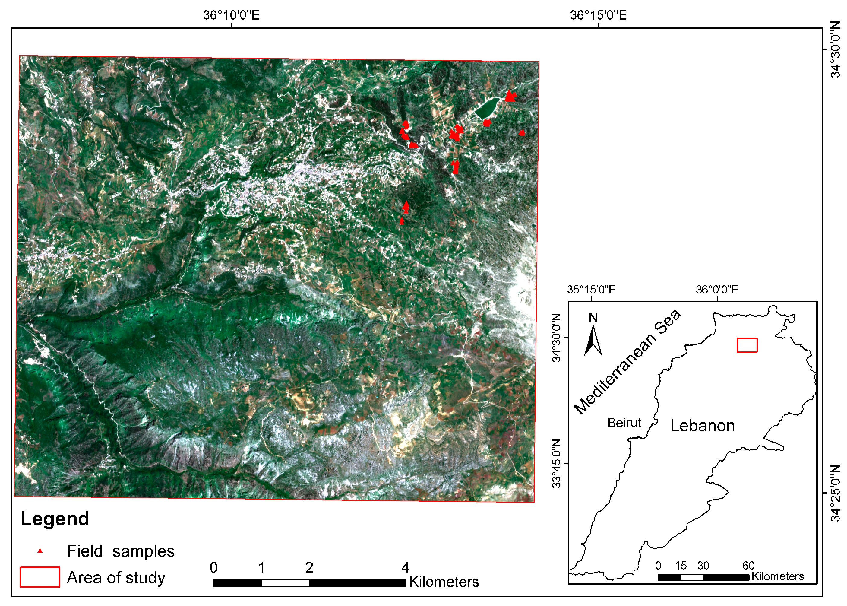
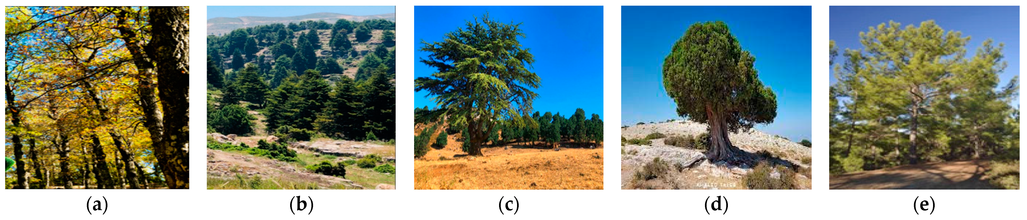
2.1. Area of Study and Field Survey
2.2. Data Type and Source
3. Methods
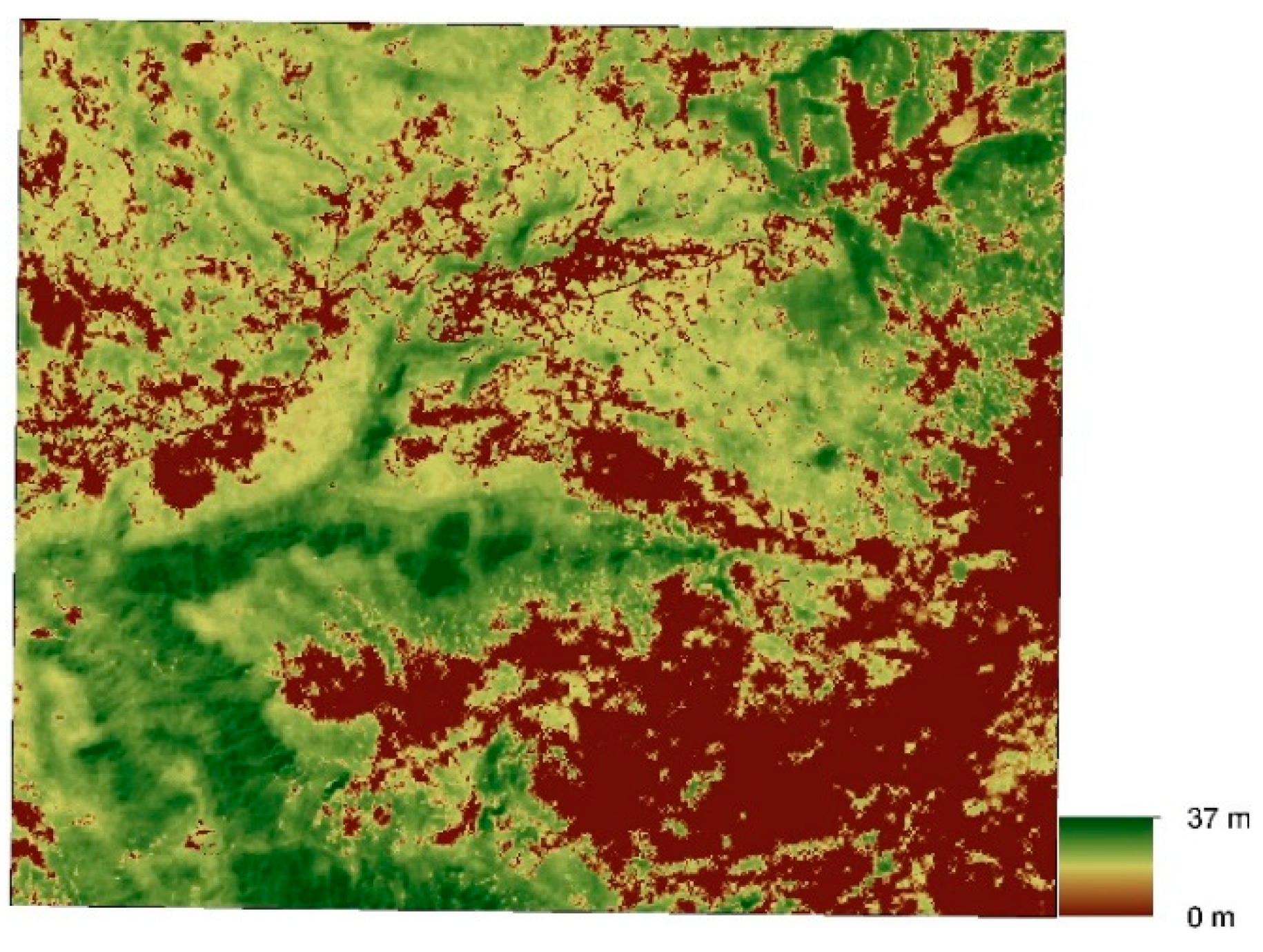
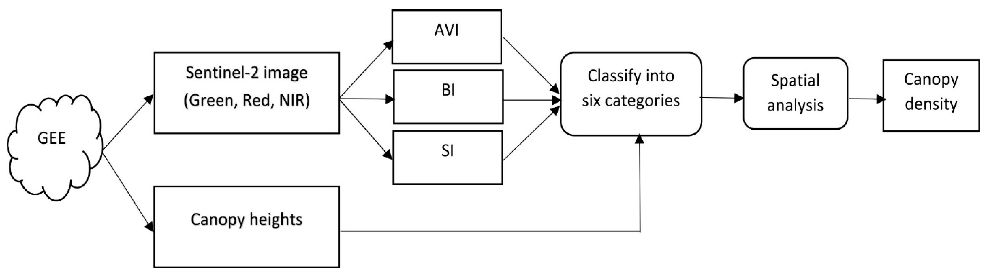
3.1. Canopy Density Model (CDM)
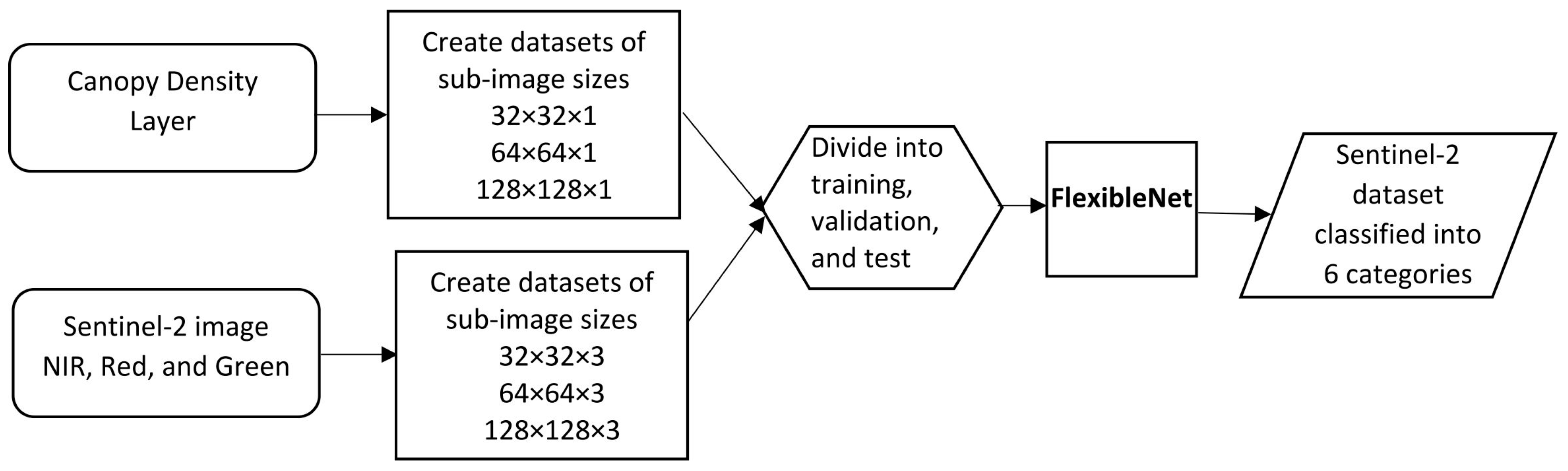
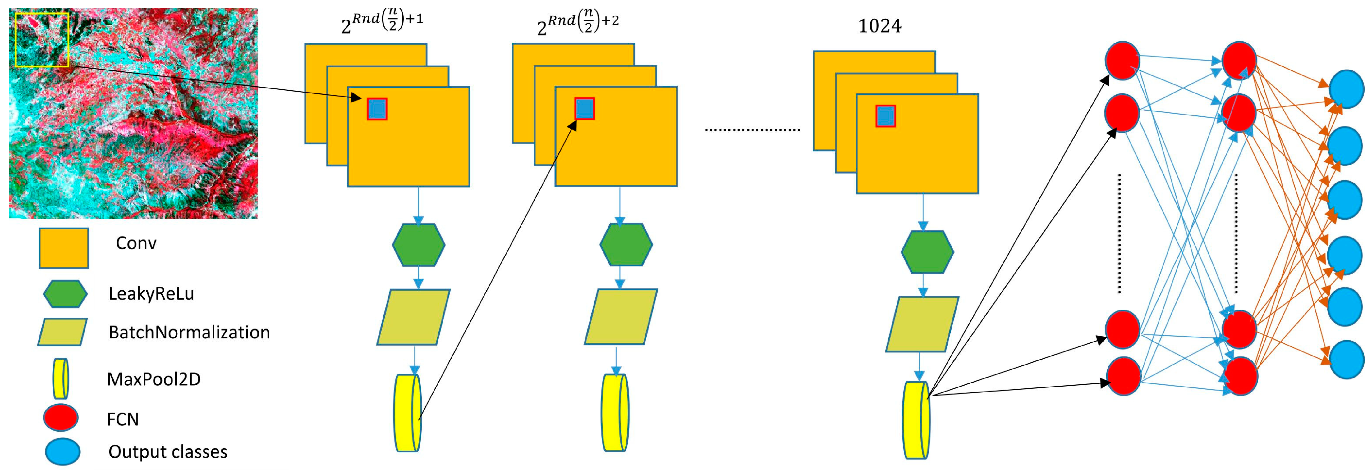
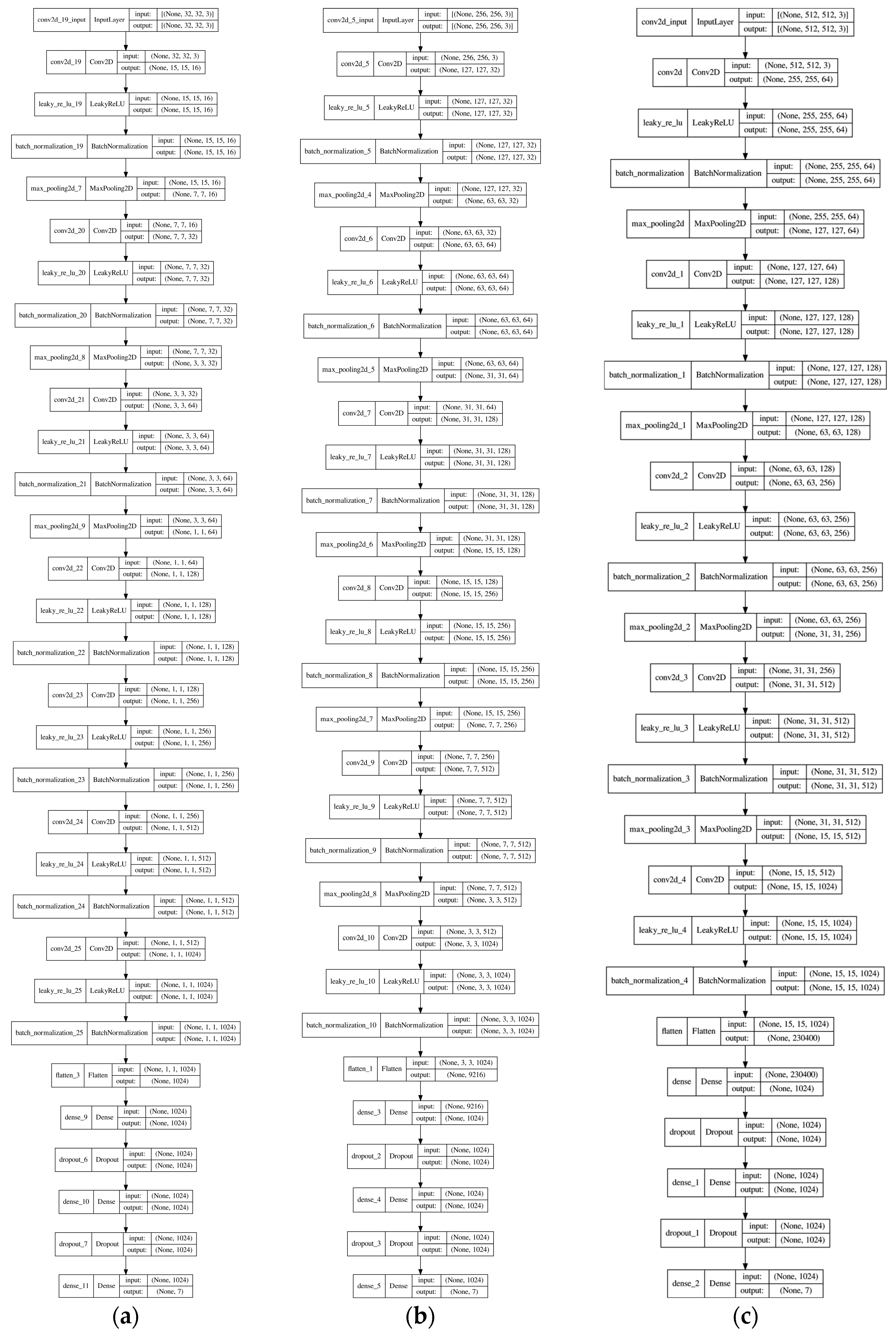
3.2. The New Lightweight Convolutional Neural Network Model (FlexibleNet)
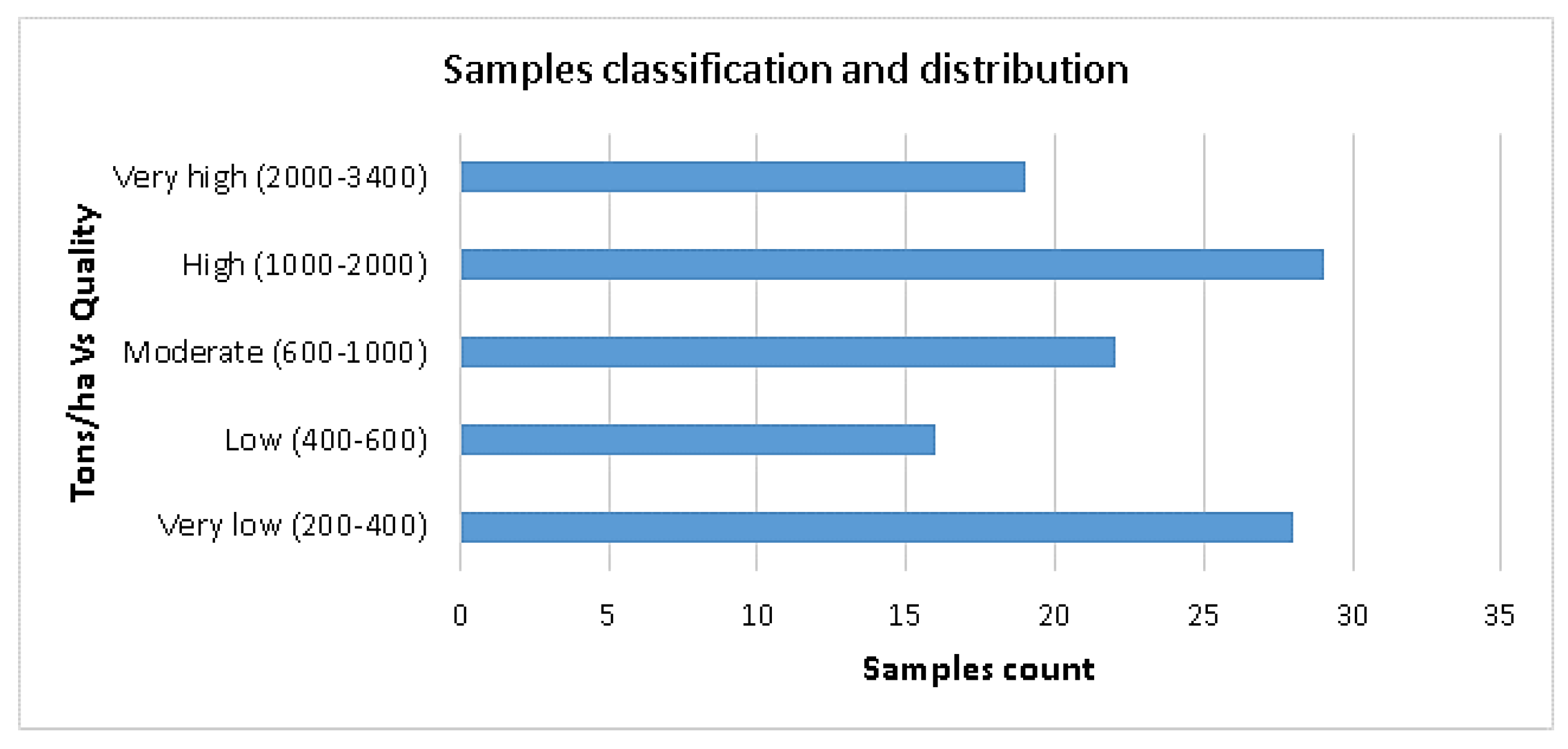
3.3. Estimating Carbon Sequestration for the Collected AGB Samples
4. Results
| Algorithm 1 A python script to classify Sentinel-2 sub-images. |
| if( (arr[i] ≤ 0) and file_exists): # it checks if the sum is less or equal to zero and if the image exists in the folder before copying it to the no carbon folder shutil.copy(filename,dest1) # copy image to no carbon folder (dest1) if((arr[i] >0 and arr[i] ≤ criteria *2) and file_exists): shutil.copy(filename,dest2) # copy to folder very low if((arr[i] > criteria *2 and arr[i] ≤ criteria *3) and file_exists): shutil.copy(filename,dest3) # copy to folder low if((arr[i] > criteria *3 and arr[i] ≤ criteria *4) and file_exists): shutil.copy(filename,dest4) # copy to folder moderate if((arr[i] > criteria *4 and arr[i] ≤ criteria *5) and file_exists): shutil.copy(filename,dest5) # copy to folder high if((arr[i] > criteria *5 and arr[i] ≤ maxval) and file_exists): shutil.copy(filename,dest6) # copy to folder very high |
5. Conclusions
Funding
Data Availability Statement
Conflicts of Interest
References
- Fradkov, A. Early History of Machine Learning. IFAC-Pap. OnLine 2020, 53, 1385–1390. [Google Scholar] [CrossRef]
- Wang, P.; Wang, L.; Leung, H.; Zhang, G. Super-Resolution Mapping Based on Spatial–Spectral Correlation for Spectral Imagery. IEEE Trans. Geosci. Remote Sens. 2021, 59, 2256–2268. [Google Scholar] [CrossRef]
- Awad, M. Cooperative evolutionary classification algorithm for hyperspectral images. J. Appl. Remote Sens. 2020, 14, 016509. [Google Scholar] [CrossRef]
- Masi, G.; Cozzolino, D.; Verdoliva, L.; Scarpa, G. Pansharpening by Convolutional Neural Networks. Remote Sens. 2016, 8, 594. [Google Scholar] [CrossRef] [Green Version]
- Girshick, R.; Donahue, J.; Darrell, T.; Malik, J. Rich Feature Hierarchies for Accurate Object Detection and Semantic Segmentation. In Proceedings of the IEEE Conference on Computer Vision and Pattern Recognition, Columbus, OH, USA, 23–28 June 2014; pp. 580–587. [Google Scholar] [CrossRef] [Green Version]
- Awad, M.M.; Lauteri, M. Self-Organizing Deep Learning (SO-UNet)—A Novel Framework to Classify Urban and Peri-Urban Forests. Sustainability 2021, 13, 5548. [Google Scholar] [CrossRef]
- Sylvain, J.; Drolet, G.; Brown, N. Mapping dead forest cover using a deep convolutional neural network and digital aerial photography. ISPRS J. Photogramm. Remote Sens. 2019, 156, 14–26. [Google Scholar] [CrossRef]
- Sarwinda, D.; Paradisa, R.; Bustamam, A.; Anggia, P. Deep Learning in Image Classification using Residual Network (ResNet) Variants for Detection of Colorectal Cancer. Procedia Comput. Sci. 2021, 179, 423–431. [Google Scholar] [CrossRef]
- Tao, J.; Gu, Y.; Sun, J.; Bie, Y.; Wang, H. Research on VGG16 convolutional neural network feature classification algorithm based on Transfer Learning. In Proceedings of the 2nd China International SAR Symposium (CISS), Shanghai, China, 3–5 November 2021; pp. 1–3. [Google Scholar] [CrossRef]
- Singh, I.; Goyal, G.; Chandel, A. AlexNet architecture based convolutional neural network for toxic comments classification. J. King Saud Univ. Comput. Inf. Sci. 2022, 34, 7547–7558. [Google Scholar] [CrossRef]
- Szegedy, C.; Liu, W.; Jia, Y.; Sermanet, P.; Reed, S.; Anguelov, D.; Erhan, D.; Vanhoucke, V.; Rabinovich, A. Going deeper with convolutions. In Proceedings of the 2015 IEEE Conference on Computer Vision and Pattern Recognition (CVPR), Boston, MA, USA, 7–12 June 2015; pp. 1–9. [Google Scholar] [CrossRef] [Green Version]
- Iandola, F.N.; Han, S.; Moskewicz, M.W.; Ashraf, K.; Dally, W.J.; Keutzer, K. SqueezeNet: AlexNet-level accuracy with 50x fewer parameters and <0.5 MB model size. arXiv 2016, arXiv:1602.07360. [Google Scholar] [CrossRef]
- Chollet, F. Xception: Deep Learning with Depth wise Separable Convolutions. In Proceedings of the IEEE Conference on Computer Vision and Pattern Recognition (CVPR), Honolulu, HI, USA, 21—26 July 2017; pp. 1800–1807. [Google Scholar] [CrossRef]
- Yuan, H.; Cheng, J.; Wu, Y.; Zeng, Z. Low-res MobileNet: An efficient lightweight network for low-resolution image classification in resource-constrained scenarios. Multimed. Tools Appl. 2022, 81, 38513–38530. [Google Scholar] [CrossRef]
- Howard, A.; Sandler, M.; Chu, G.; Chen, L.C.; Chen, B.; Tan, M.; Wang, W.; Zhu, Y.; Pang, R.; Vasudevan, V. Searching for MobileNetV3. In Proceedings of the IEEE International Conference on Computer Vision, Seoul, Republic of Korea, 27–28 October 2019; pp. 1314–1324. [Google Scholar] [CrossRef]
- Ma, N.; Zhang, X.; Zheng, H.T.; Sun, J. Shufflenet v2: Practical guidelines for efficient CNN architecture design. In Proceedings of the European conference on computer vision (ECCV), Munich, Germany, 8–14 September 2018; pp. 116–131. [Google Scholar] [CrossRef]
- Tan, M.; Le, Q.V. (2019) EfficientNet: Rethinking Model Scaling for Convolutional Neural Networks. In Proceedings of the 36th International Conference on Machine Learning, Long Beach, CA, USA, 10–19 June 2019; pp. 6105–6114. [Google Scholar]
- Sarker, I.H. Deep Learning: A Comprehensive Overview on Techniques, Taxonomy, Applications and Research Directions. SN Comput. Sci. 2021, 2, 420. [Google Scholar] [CrossRef] [PubMed]
- Zhou, Y.; Bai, Y.; Bhattacharyya, S.; Huttunen, H. Elastic Neural Networks for Classification. In Proceedings of the 2 IEEE International Conference on Artificial Intelligence Circuits and Systems (AICAS), Taiwan, China, 18–20 March 2019; pp. 251–255. [Google Scholar] [CrossRef] [Green Version]
- Bai, Y.; Bhattacharyya, S.; Happonen, A.; Huttunen, H. Elastic Neural Networks: A Scalable Framework for Embedded Computer Vision. In Proceedings of the 26th European Signal Processing Conference (EUSIPCO), Rome, Italy, 3–7 September 2018; pp. 1472–1476. [Google Scholar] [CrossRef] [Green Version]
- Yu, D.; Xu, Q.; Guo, H.; Zhao, C.; Lin, Y.; Li, D. An Efficient and Lightweight Convolutional Neural Network for Remote Sensing Image Scene Classification. Sensors 2020, 20, 1999. [Google Scholar] [CrossRef] [PubMed]
- Chen, Y.; Chen, X.; Lin, J.; Pan, R.; Cao, T.; Cai, J.; Yu, D.; Cernava, T.; Zhang, X. DFCANet: A Novel Lightweight Convolutional Neural Network Model for Corn Disease Identification. Agriculture 2022, 12, 2047. [Google Scholar] [CrossRef]
- Kawamiya, M.; Hajima, T.; Tachiiri, K.; Watanabe, S.; Yokohata, T. Two decades of Earth system modeling with an emphasis on Model for Interdisciplinary Research on Climate (MIROC). Prog. Earth Planet. Sci. 2020, 7, 64. [Google Scholar] [CrossRef]
- Deng, L.; Zhu, G.Y.; Tang, Z.S.; Shangguan, Z.P. Global patterns of the effects of land-use changes on soil carbon stocks. Glob. Ecol. Conserv. 2016, 5, 127–138. [Google Scholar] [CrossRef] [Green Version]
- Food And Agriculture Organization of the United Nations (FAO). Global Forest Resources Assessment 2015—How Are the World’s Forests Changing? 2nd ed.; FAO: Rome, Italy, 2016; p. 54. [Google Scholar]
- Bernal, B.; Murray, L.T.; Pearson, T.R.H. Global carbon dioxide removal rates from forest landscape restoration activities. Carbon Balance Manag. 2018, 13, 22. [Google Scholar] [CrossRef]
- Kim, H.; Kim, Y.H.; Kim, R.; Park, H. Reviews of forest carbon dynamics models that use empirical yield curves: CBM-CFS3, CO2FIX, CASMOFOR, EFISCEN. For. Sci. Technol. 2015, 11, 212–222. [Google Scholar] [CrossRef]
- Liu, F.; Tan, C.; Zhang, G.; Liu, J.X. Single-wood parameters and biomass airborne LiDAR estimation of Larix olgensis. Trans. Chin. Soc. Agric. 2013, 44, 219–224. [Google Scholar]
- Lizuka, K.; Tateishi, R. Estimation of CO2 Sequestration by the Forests in Japan by Discriminating Precise Tree Age Category using Remote Sensing Techniques. Remote Sens. 2015, 7, 15082–15113. [Google Scholar] [CrossRef] [Green Version]
- Castro-Magnani, M.; Sanchez-Azofeifa, A.; Metternicht, G.; Laakso, K. Integration of remote-sensing based metrics and econometric models to assess the socio-economic contributions of carbon sequestration in unmanaged tropical dry forests. Environ. Sustain. Indic. 2021, 9, 100100. [Google Scholar] [CrossRef]
- Costanza, R.; de Groot, R.; Braat, L.; Kubiszewski, I.; Fioramonti, L.; Sutton, P.; Farber, S.; Grasso, M. Twenty years of ecosystem services: How far have we come and how far do we still need to go? Ecosyst. Serv. 2017, 28, 1–16. [Google Scholar] [CrossRef]
- Hao, H.; Li, W.; Zhao, X.; Chang, Q.; Zhao, P. Estimating the Aboveground Carbon Density of Coniferous Forests by Combining Airborne LiDAR and Allometry Models at Plot Level. Front. Plant Sci. 2019, 10, 917. [Google Scholar] [CrossRef] [PubMed] [Green Version]
- Kanniah, K.; Muhamad, N.; Kang, C. Remote sensing assessment of carbon storage by urban forest, IOP Conference Series: Earth and Environmental Science. In Proceedings of the 8th International Symposium of the Digital Earth (ISDE8), Kuching, Malaysia, 26–29 August 2013; Volume 18. [Google Scholar]
- Uniyal, S.; Purohit, S.; Chaurasia, K.; Rao, S.; Amminedu, E. Quantification of carbon sequestration by urban forest using Landsat 8 OLI and machine learning algorithms in Jodhpur, India. Sci. Direct Urban For. Urban Green. 2022, 67, 127445. [Google Scholar] [CrossRef]
- Foody, G.; Mathur, A. A relative evaluation of multiclass image classification by support vector machines. IEEE Trans. Geosci. Remote Sens. 2004, 42, 1335–1343. [Google Scholar] [CrossRef] [Green Version]
- Gwal, S.; Singh, S.; Gupta, S.; Anand, S. Understanding forest biomass and net primary productivity in Himalayan ecosystem using geospatial approach. Model. Earth Syst. Environ. 2020, 6, 10. [Google Scholar] [CrossRef]
- Kimes, D.; Nelson, R.; Manry, M.; Fung, A. Review article: Attributes of neural networks for extracting continuous vegetation variables from optical and radar measurements. Int. J. Remote Sens. 1998, 19, 2639–2663. [Google Scholar] [CrossRef]
- Sagi, O.; Rokach, L. Approximating XGBoost with an interpretable decision tree. Inf. Sci. 2021, 572, 522–542. [Google Scholar] [CrossRef]
- Zhang, F.; Tian, X.; Zhang, H.; Jiang, M. Estimation of Aboveground Carbon Density of Forests Using Deep Learning and Multisource Remote Sensing. Remote Sens. 2022, 14, 3022. [Google Scholar] [CrossRef]
- Liu, W.; Wang, Z.; Liu, X.; Zeng, N.; Liu, Y.; Alsaadi, F.E. A survey of deep neural network architectures and their applications. Neurocomputing 2017, 234, 11–26. [Google Scholar] [CrossRef]
- LeCun, Y.; Bengio, Y.; Hinton, G. Deep learning. Nature 2015, 521, 436–444. [Google Scholar] [CrossRef]
- Li, J.; Roy, D.A. global analysis of Sentinel-2A, Sentinel-2B and Landsat-8 data revisit intervals and implications for terrestrial monitoring. Remote Sens. 2017, 9, 902. [Google Scholar] [CrossRef] [Green Version]
- Lang, N.; Jetz, W.; Schindler, K.; Wegner, A. High-resolution canopy height model of the Earth. arXiv 2022, arXiv:2204.08322. [Google Scholar]
- Abdollahnejad, A.; Panagiotidis, D.; Surový, P. Forest canopy density assessment using different approaches—Review. J. For. Sci. 2017, 63, 107–116. [Google Scholar]
- Chen, J.; Yang, S.; Li, H.; Zhang, B.; Lv, J. Research on Geographical Environment Unit Division Based on The Method of Natural Breaks (Jenks), The International Archives of the Photogrammetry. Remote Sens. Spat. Inf. Sci. 2013, 3, 47–50, 2013 ISPRS/IGU/ICA Joint Workshop on Borderlands Modelling and Understanding for Global Sustainability 2013, Beijing, China. [Google Scholar]
- Mamoshina, P.; Vieira, A.; Putin, E.; Zhavoronkov, A. Applications of Deep Learning in Biomedicine. Mol. Pharm. 2016, 13, 1445–1454. [Google Scholar] [CrossRef]
- Khan, A.; Sohail, A.; Zahoora, U.; Qureshi, A.S. A Survey of the Recent Architectures of Deep Convolutional Neural Networks. Artif. Intell. Rev. 2020, 53, 5455–5516. [Google Scholar] [CrossRef]
- Xu, B.; Wang, N.; Chen, T.; Li, M. Empirical Evaluation of Rectified Activations in Convolutional Network. arXiv 2015, arXiv:1505.00853. [Google Scholar]
- Josephine, V.L.; Nirmala, A.P.; Allur, V. Impact of Hidden Dense Layers in Convolutional Neural Network to enhance Performance of Classification Model, IOP Conference Series: Materials Science and Engineering. In Proceedings of the 4th International Conference on Emerging Technologies in Computer Engineering: Data Science and Blockchain Technology (ICETCE 2021), Jaipur, India, 3–4 February 2021; Volume 1131. [Google Scholar]
- Lee, D.; Park, C.; Tomlin, D. Effects of land-use-change scenarios on terrestrial carbon stocks in South Korea. Landsc. Ecol. Eng. 2015, 11, 47–59. [Google Scholar] [CrossRef]
- Scott, D. Sturges’ rule. WIREs Comput. Stat. 2009, 1, 303–306. [Google Scholar] [CrossRef]
- Belavkin, R.; Pardalos, P.; Principe, J. Value of Information in the Binary Case and Confusion Matrix. Phys. Sci. Forum 2022, 5, 5008. [Google Scholar] [CrossRef]
- Bottou, L.; Bousquet, O. The Tradeoffs of Large Scale Learning. In Optimization for Machine Learning; Sra, S., Nowozin, S., Stephen, J.W., Eds.; MIT Press: Cambridge, UK, 2012; pp. 351–368. ISBN 978-0-262-01646-9. [Google Scholar]
- Asif, A.; Waris, A.; Gilani, S.; Jamil, M.; Ashraf, H.; Shafique, M.; Niazi, I.K. Performance Evaluation of Convolutional Neural Network for Hand Gesture Recognition Using EMG. Sensors 2020, 20, 1642. [Google Scholar] [CrossRef] [PubMed] [Green Version]
- Sandler, M.; Howard, A.; Zhu, M.; Zhmoginov, A.; Chen, L.C. MobileNetV2: Inverted Residuals and Linear Bottlenecks. In Proceedings of the IEEE/CVF Conference on Computer Vision and Pattern Recognition, Salt Lake City, UT, USA, 18–23 June 2018; pp. 4510–4520. [Google Scholar] [CrossRef]
- Goodfellow, I.; Bengio, Y.; Courville, A. Deep Learning (Adaptive Computation and Machine Learning Series); The MIT Press: Cambridge, MA, USA, 2016; p. 800. [Google Scholar]


| Type | Number of Samples | Average DBH (cm) | Average Height (Meters) |
|---|---|---|---|
| Quercus Cerris | 17 | 119 | 15 |
| Pinus brutia | 19 | 125 | 12 |
| Abies cilicica | 46 | 237 | 17 |
| Juniperus excelsa | 32 | 225 | 8 |
| Type of Forest | Bulk Density (Bd) (Tons/m³) | Biomass Expansion (Be) | Carbon Content (Cc) |
|---|---|---|---|
| Coniferous | 0.47 | 1.651 | 0.5 |
| Deciduous | 0.80 | 1.720 | 0.5 |
| Mixed | 0.635 | 1.685 | 0.5 |
| Measured/Estimated | Very Low | Low | Moderate | High | Very High |
|---|---|---|---|---|---|
| Very low | 23 | 2 | 1 | 2 | 0 |
| Low | 1 | 15 | 0 | 0 | 0 |
| Moderate | 0 | 1 | 21 | 0 | 0 |
| High | 1 | 1 | 0 | 27 | 0 |
| Very high | 0 | 0 | 0 | 0 | 19 |
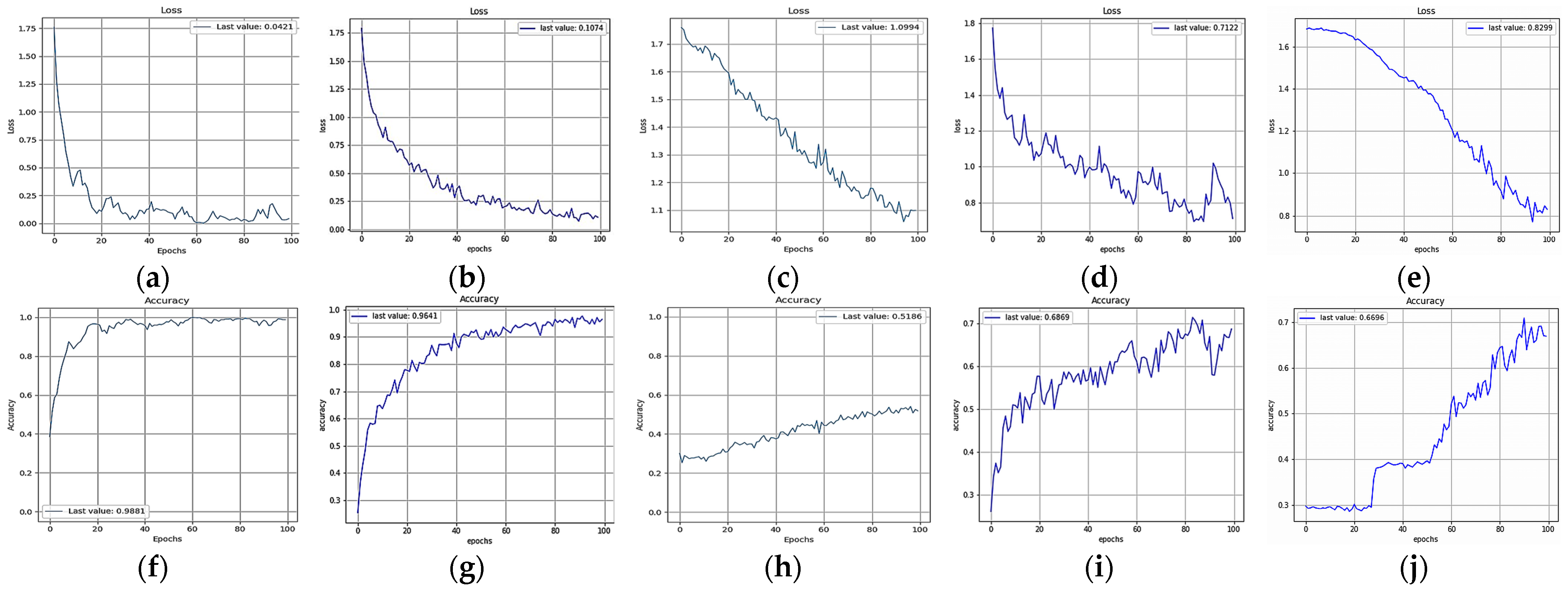
| Model Name | Number of Parameters (Millions) | Time Requirement (Minutes) | Accuracy % | Lowest Loss Value |
|---|---|---|---|---|
| FlexibleNet | 5.52 | 13.3 | 98.81 | 0.042 |
| ResNet50 | 26.38 | 77 | 96.41 | 0.1074 |
| EfficientNetB5 | 31.30 | 28.4 | 52 | 1.1 |
| MobileNetV3-Large | 6.23 | 13.3 | 68.69 | 0.7122 |
| Xception | 21.58 | 62 | 66.96 | 0.83 |
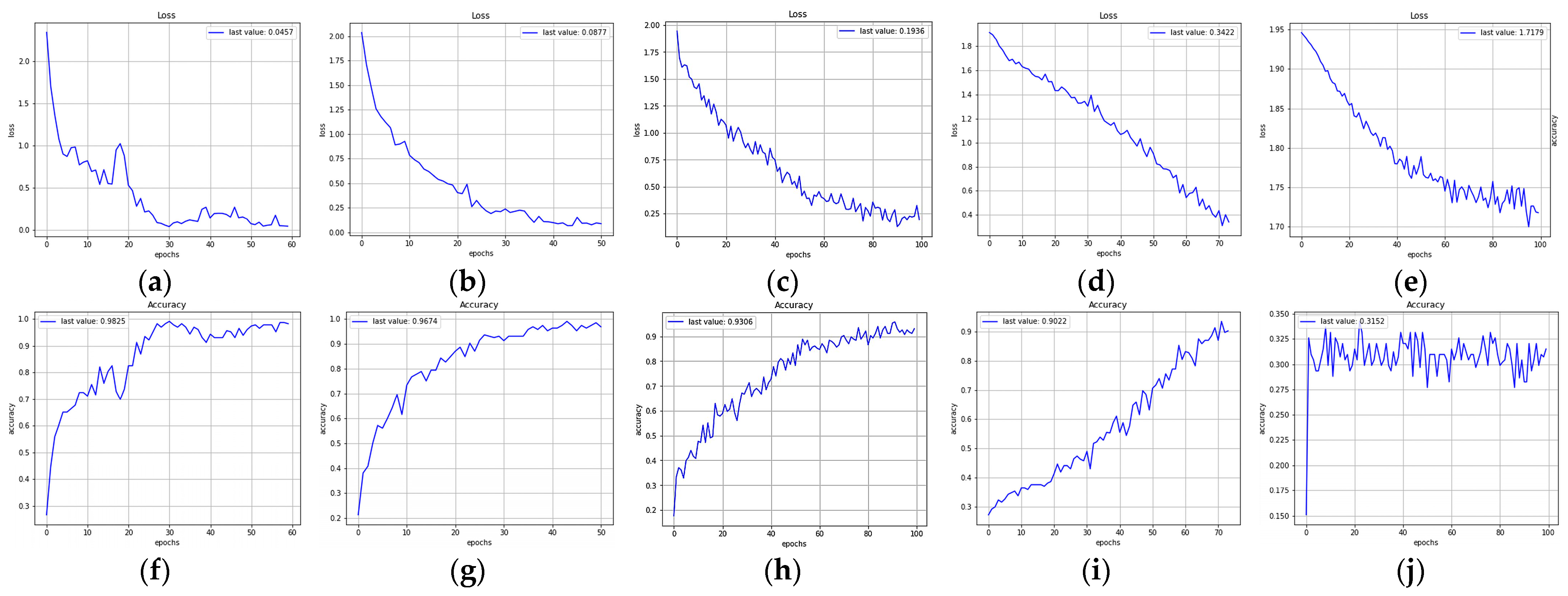
| Model Name | Number of Parameters (Millions) | Time Requirement (Minutes) | Accuracy % | Lowest Loss Value | Total Iterations |
|---|---|---|---|---|---|
| FlexibleNet | 8.4 | 5 | 98.25 | 0.0457 | 60 |
| ResNet50 | 32.6 | 13 | 96.74 | 0.0877 | 51 |
| EfficientNetB5 | 32.9 | 40 | 93.06 | 0.1936 | 100 |
| MobileNetV3-Large | 6.23 | 4 | 90.22 | 0.3422 | 74 |
| Xception | 21.58 | 22 | 31.52 | 1.718 | 100 |
| Model Name | Number of Parameters (Millions) | Time Requirement (Minutes) | Accuracy % | Lowest Loss Value | Total Iterations |
|---|---|---|---|---|---|
| FlexibleNet | 8.4 | 0.8 | 98.25 | 0.0657 | 24 |
| ResNet50 | 57.8 | 7.7 | 86.87 | 0.2953 | 23 |
| EfficientNet | 62.7 | 6 | 70.09 | 0.9102 | 11 |
| MobileNetV3-Large | 6.23 | 8.1 | 96.97 | 0.0951 | 68 |
| Xception | 55.1 | 20.53 | 90.91 | 0.2523 | 56 |
Disclaimer/Publisher’s Note: The statements, opinions and data contained in all publications are solely those of the individual author(s) and contributor(s) and not of MDPI and/or the editor(s). MDPI and/or the editor(s) disclaim responsibility for any injury to people or property resulting from any ideas, methods, instructions or products referred to in the content. |
© 2023 by the author. Licensee MDPI, Basel, Switzerland. This article is an open access article distributed under the terms and conditions of the Creative Commons Attribution (CC BY) license (https://creativecommons.org/licenses/by/4.0/).
Share and Cite
Awad, M.M. FlexibleNet: A New Lightweight Convolutional Neural Network Model for Estimating Carbon Sequestration Qualitatively Using Remote Sensing. Remote Sens. 2023, 15, 272. https://doi.org/10.3390/rs15010272
Awad MM. FlexibleNet: A New Lightweight Convolutional Neural Network Model for Estimating Carbon Sequestration Qualitatively Using Remote Sensing. Remote Sensing. 2023; 15(1):272. https://doi.org/10.3390/rs15010272
Chicago/Turabian StyleAwad, Mohamad M. 2023. "FlexibleNet: A New Lightweight Convolutional Neural Network Model for Estimating Carbon Sequestration Qualitatively Using Remote Sensing" Remote Sensing 15, no. 1: 272. https://doi.org/10.3390/rs15010272