

Evaluation of InSAR Tropospheric Correction by Using Efficient WRF Simulation with ERA5 for Initialization

Abstract
:
1. Introduction
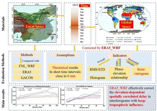
2. Experiment Design and Materials
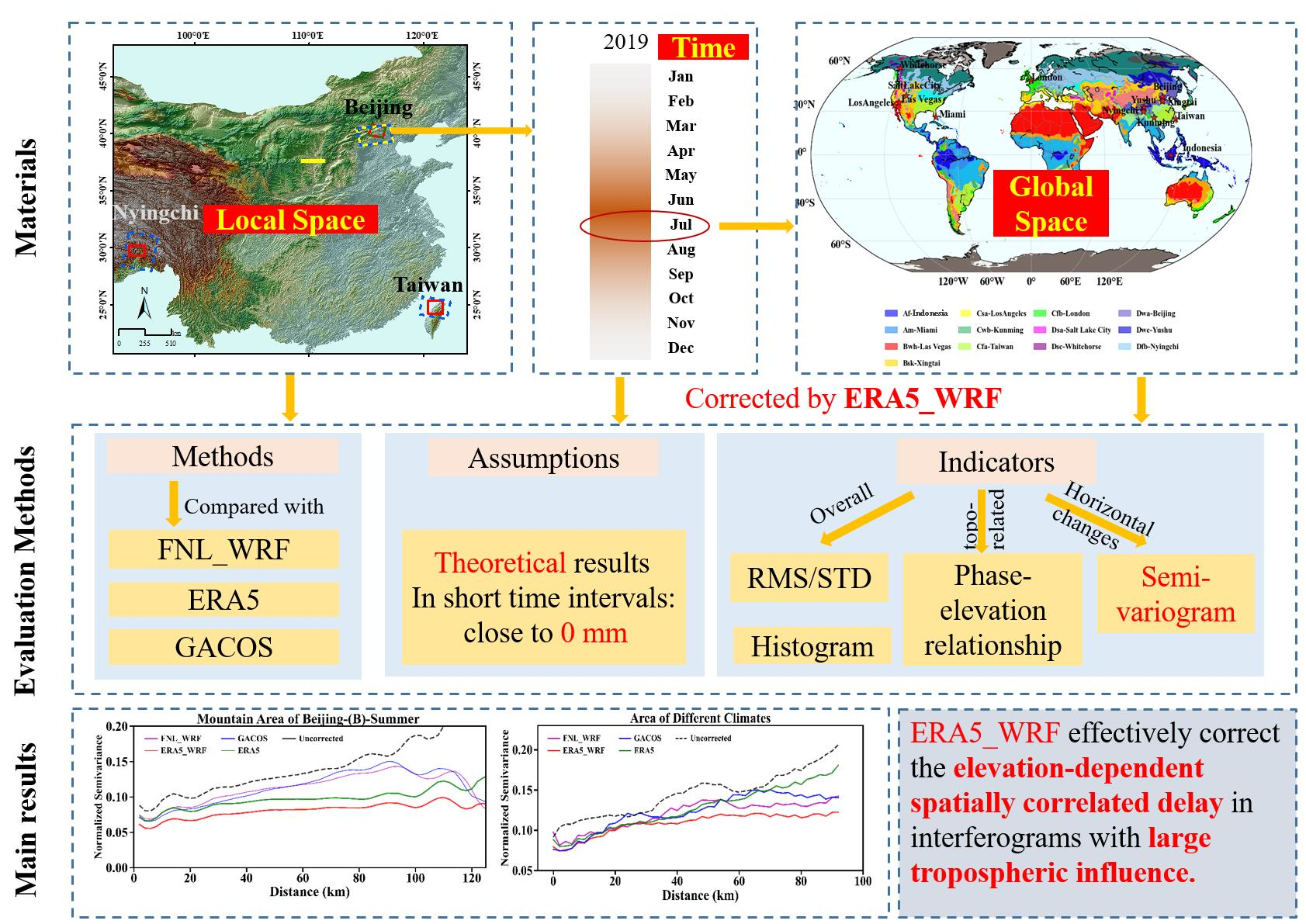
2.1. Local Space-Typical Regions with Different Tropospheric Properties
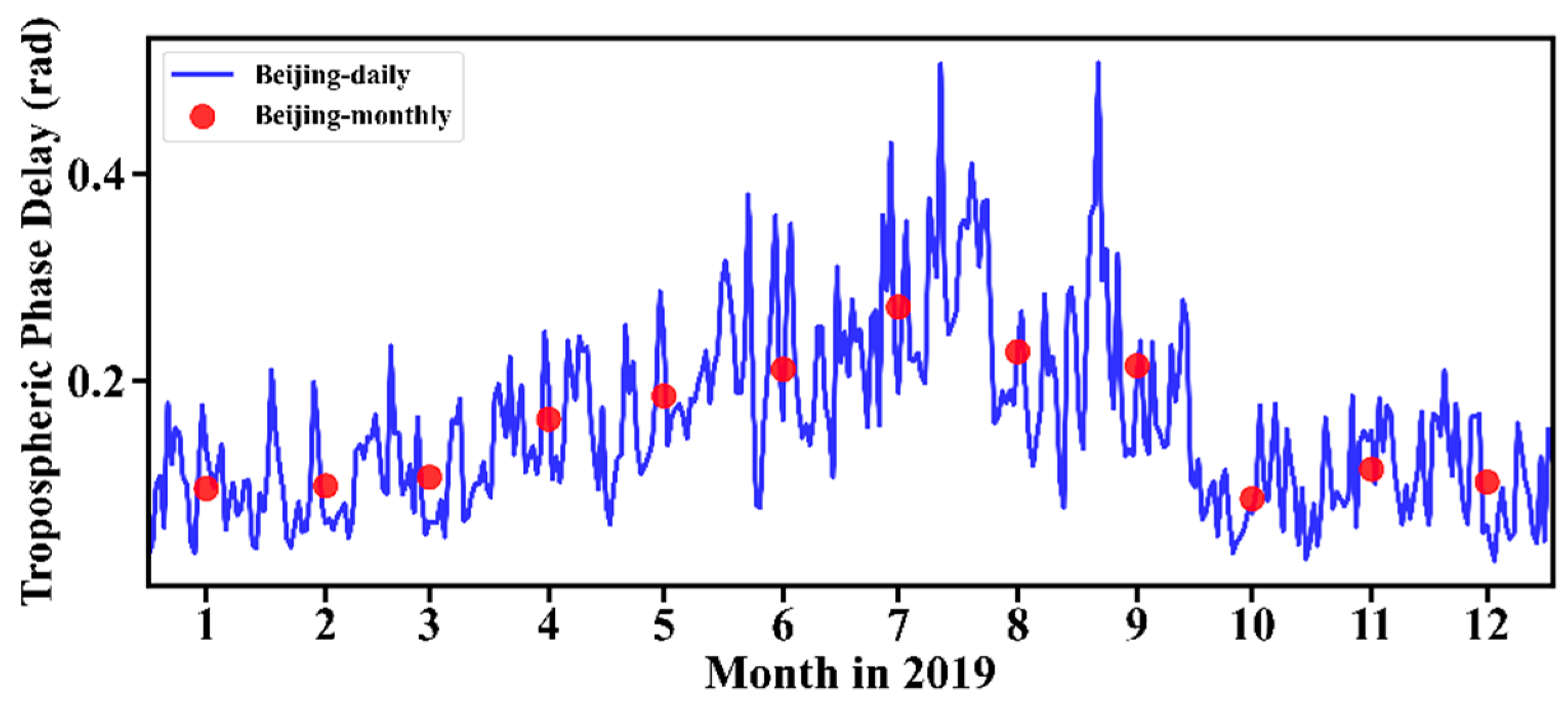
2.2. Time-Seasonality Effects
2.3. Correction Evaluation
- (1)
- Local space
- (2)
- Time
3. Methods
3.1. Calculation Principle of Tropospheric Phase Delay
3.2. WRF Model
3.2.1. WRF Configuration
3.2.2. WRF Simulation
- (1)
- WRF preprocessing
- (2)
- WRF simulation
3.3. Methods for Comparison
3.4. InSAR Processing
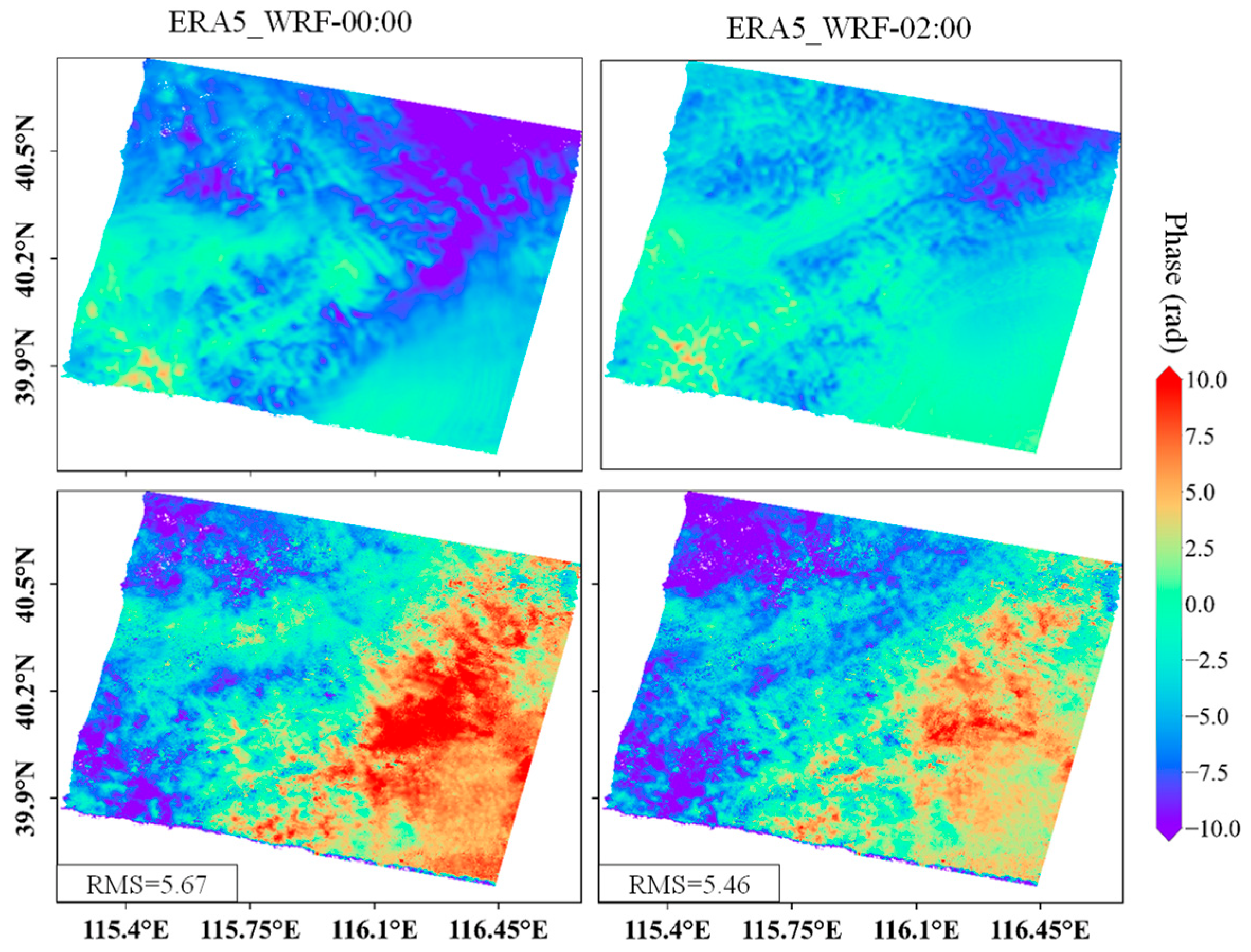
4. Results
4.1. Local Space-Typical Regions with Different Tropospheric Conditions
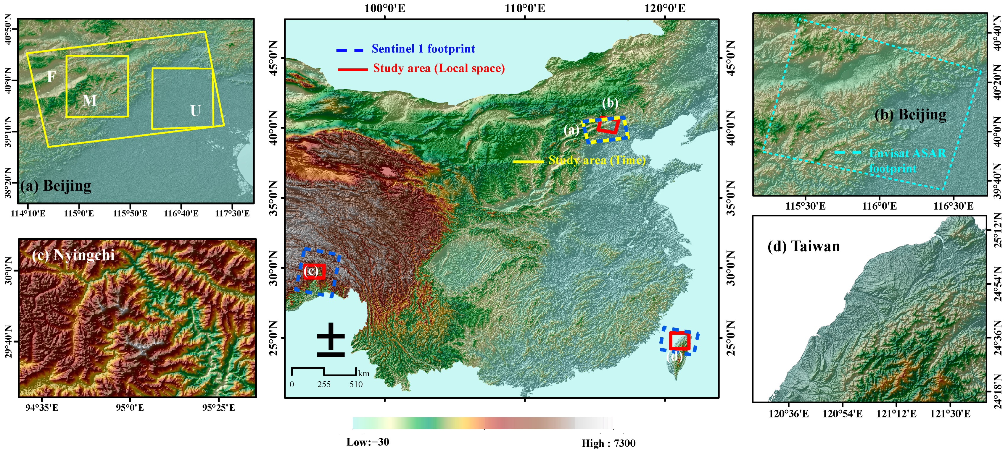
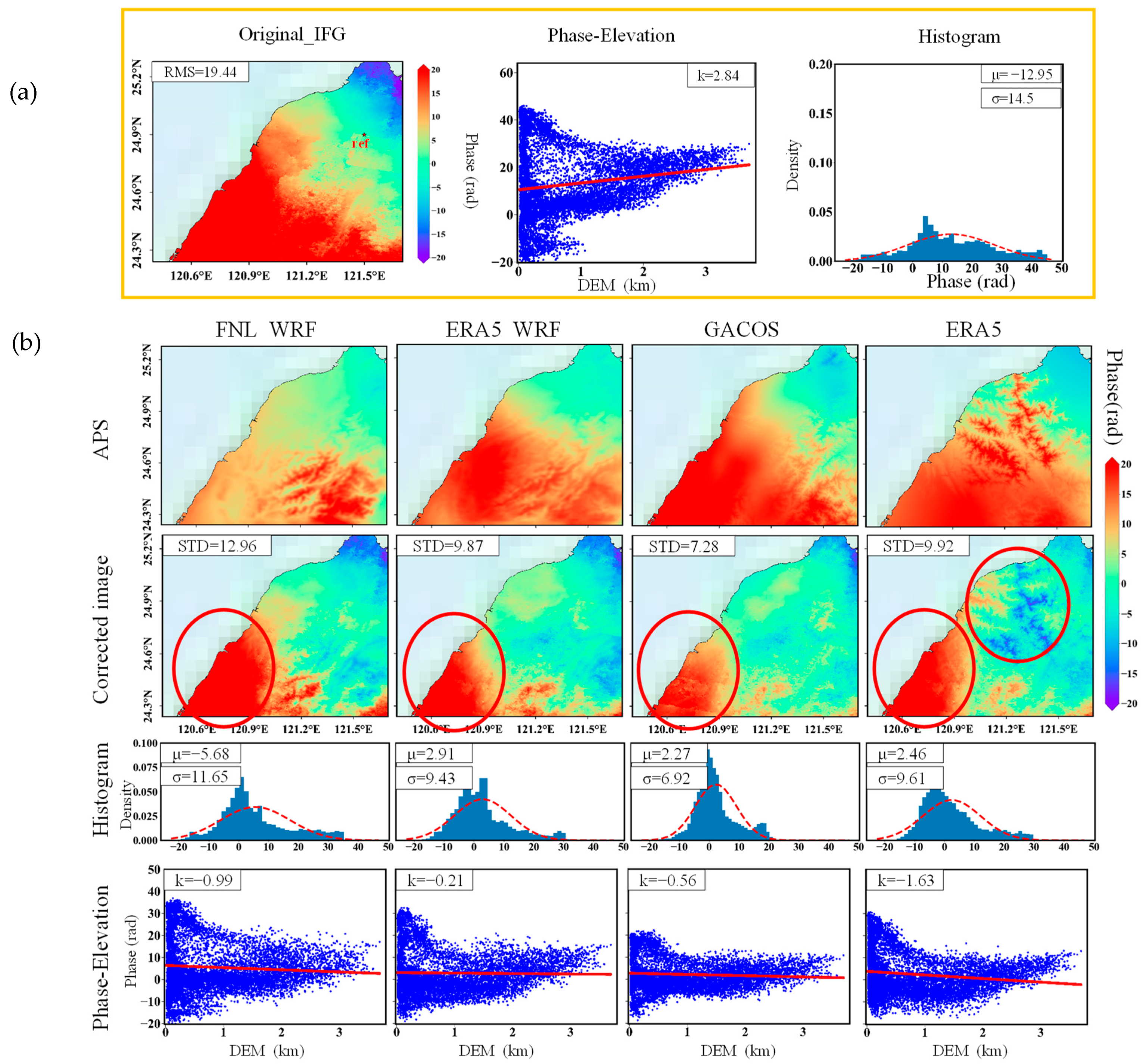
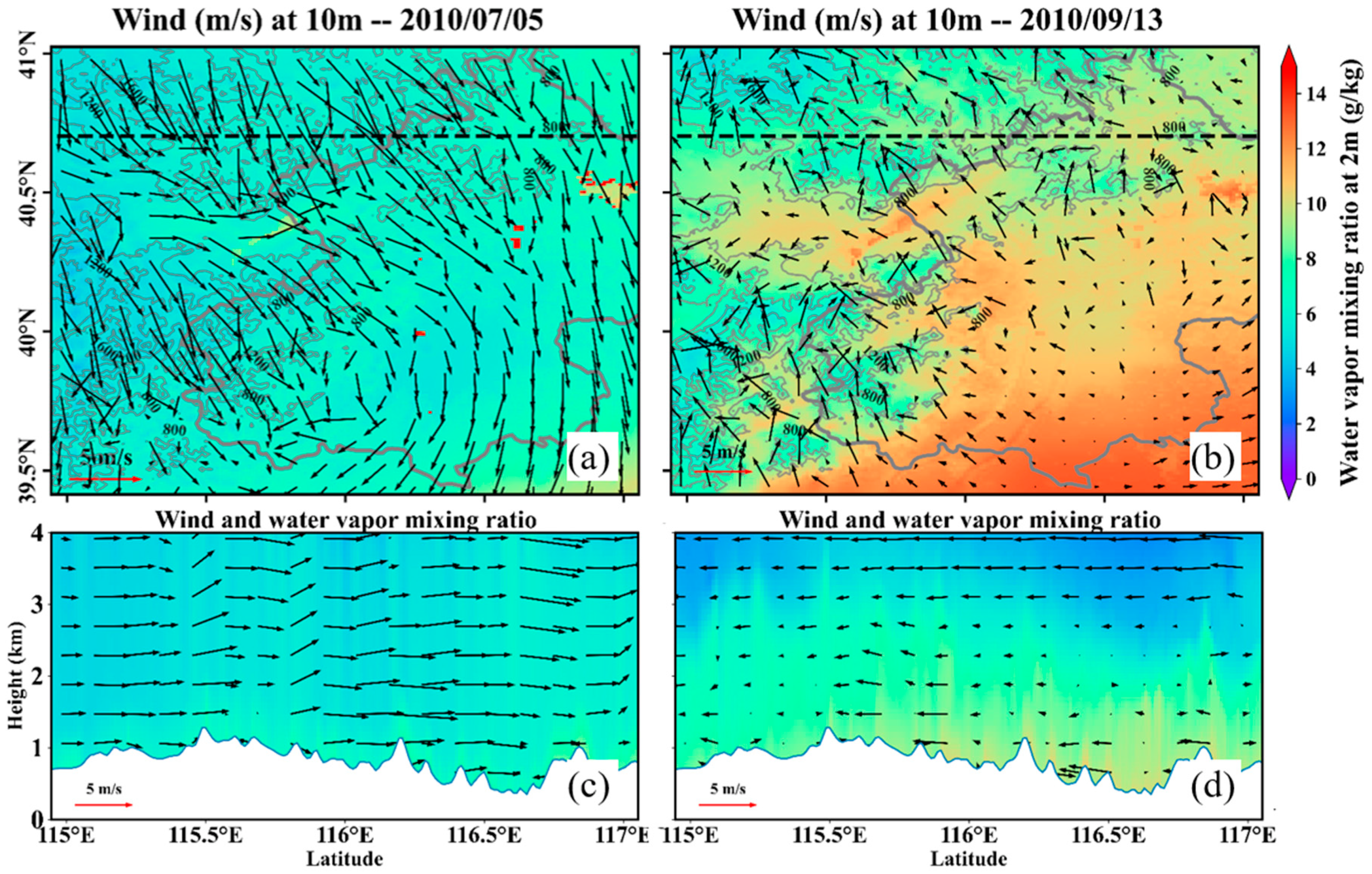
4.1.1. Beijing
- (1)
- RMS errors
- (2)
- Histogram
- (3)
- The phase–elevation correlation coefficient
- (4)
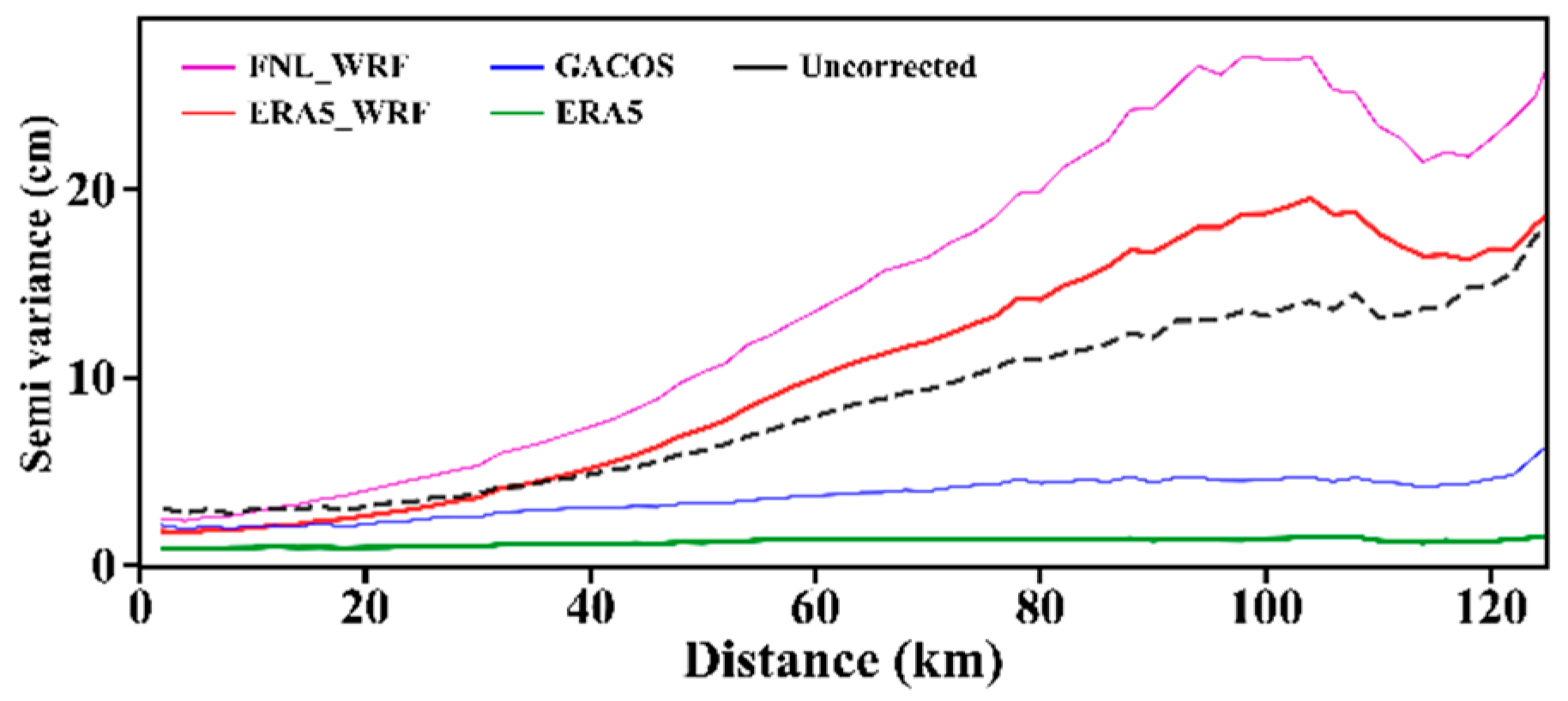
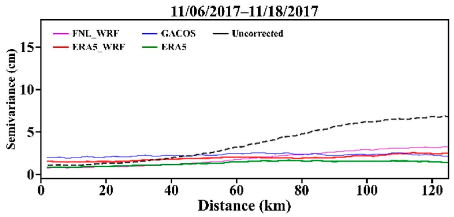
- Semi-variogram
- (5)
- Summary
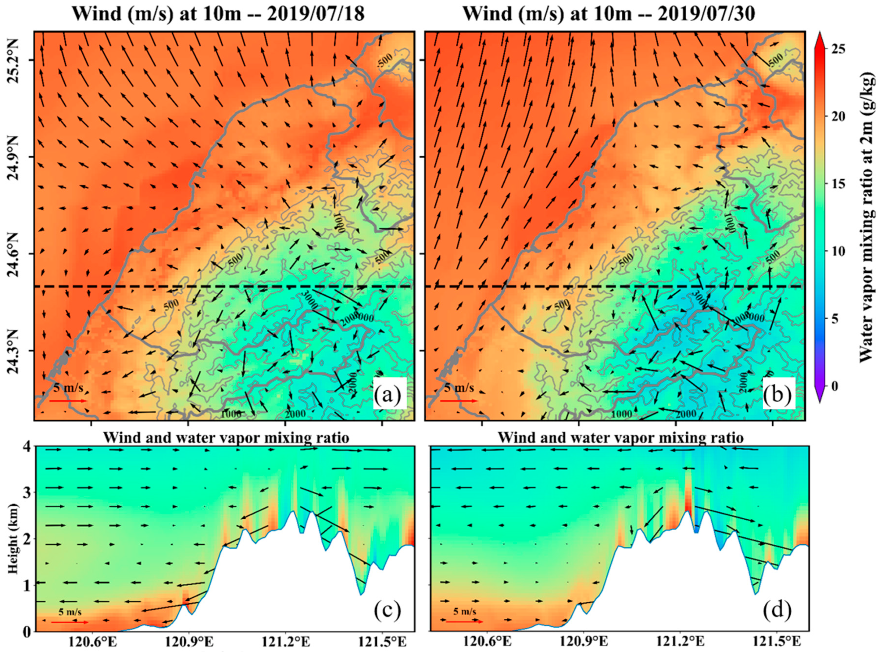
4.1.2. Taiwan
- (1)
- RMS errors
- (2)
- Residuals distribution and histogram
- (3)
- The phase–elevation correlation coefficient
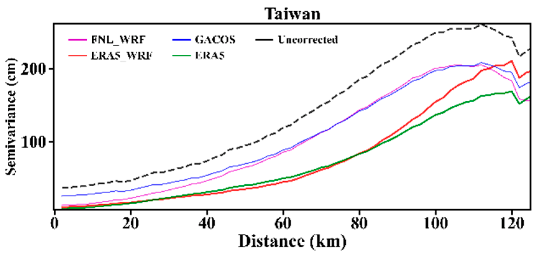
- (4)
- Semi-variograms
- (5)
- Summary
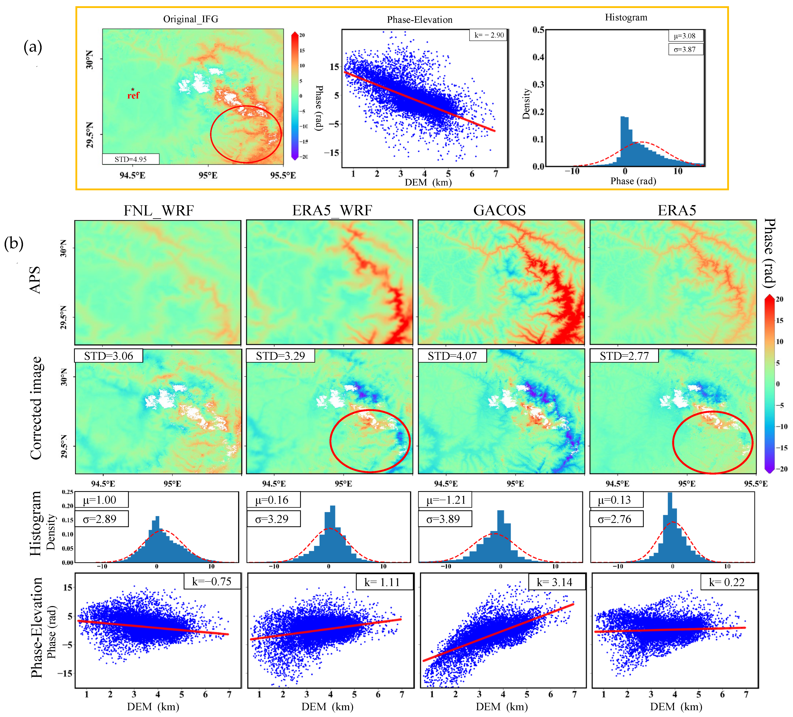
4.1.3. Nyingchi
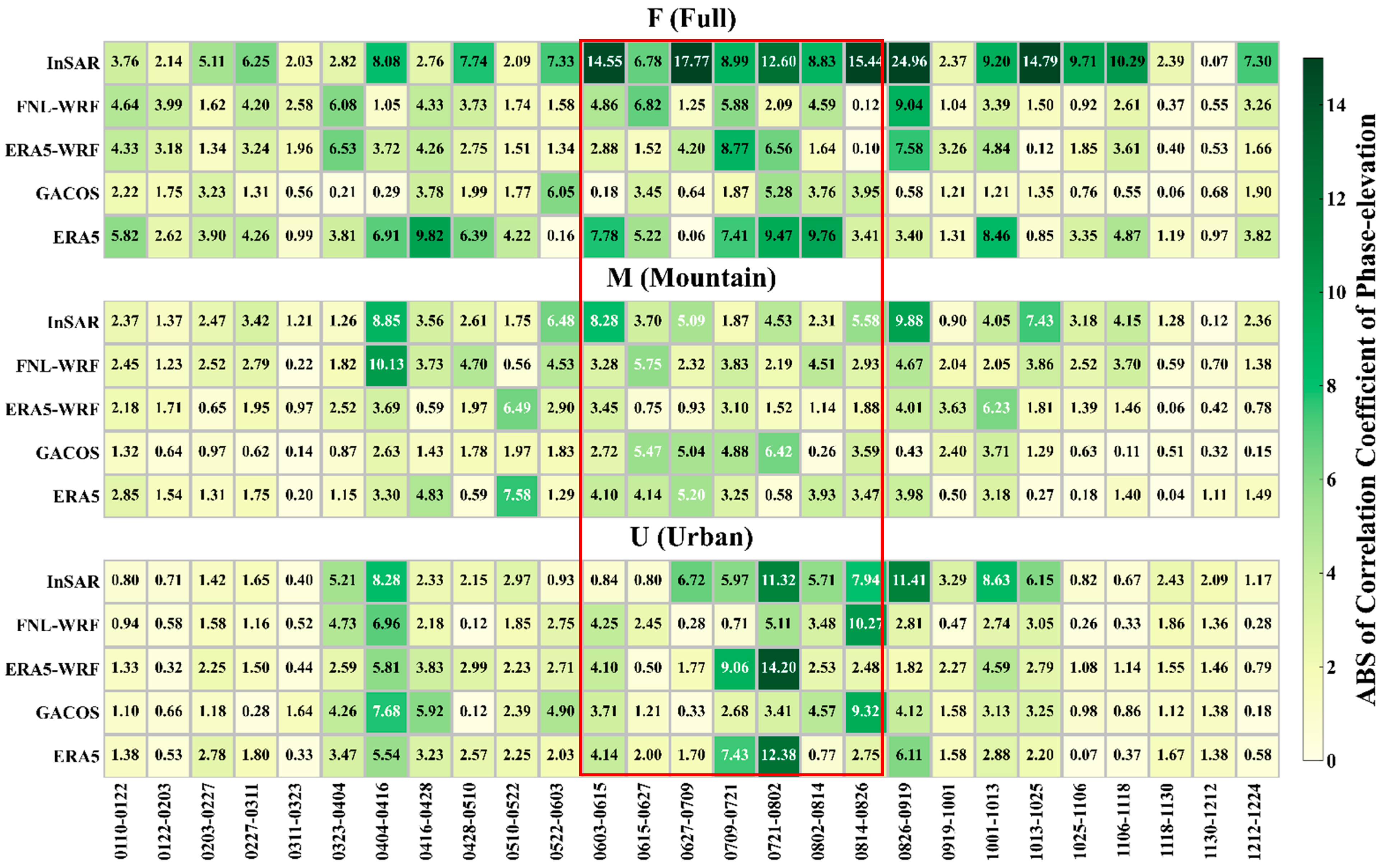
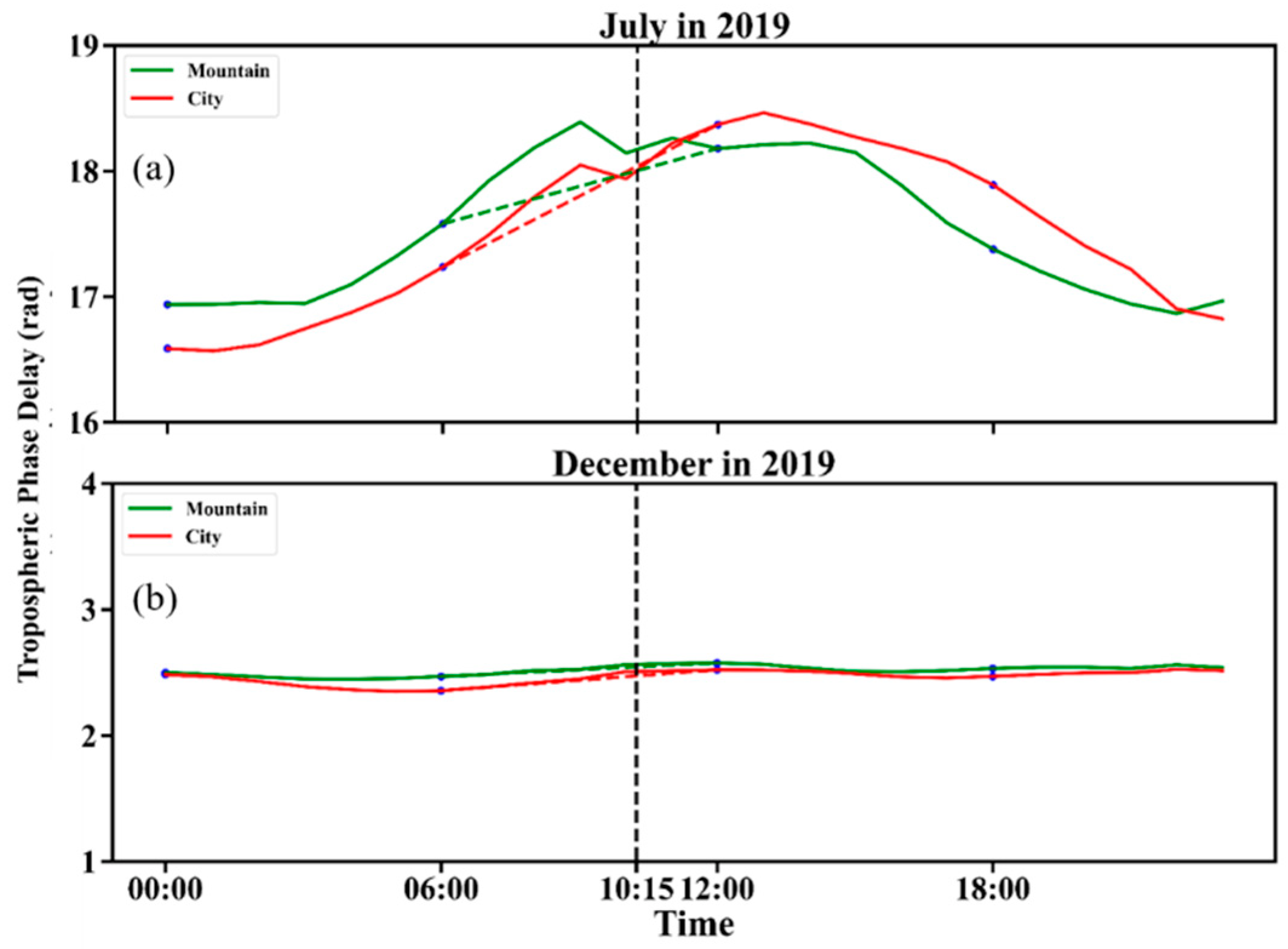
4.2. Time-Seasonality Effects
- (1)
- STD errors
- (2)
- The absolute value of the phase–elevation correlation coefficient
- (3)
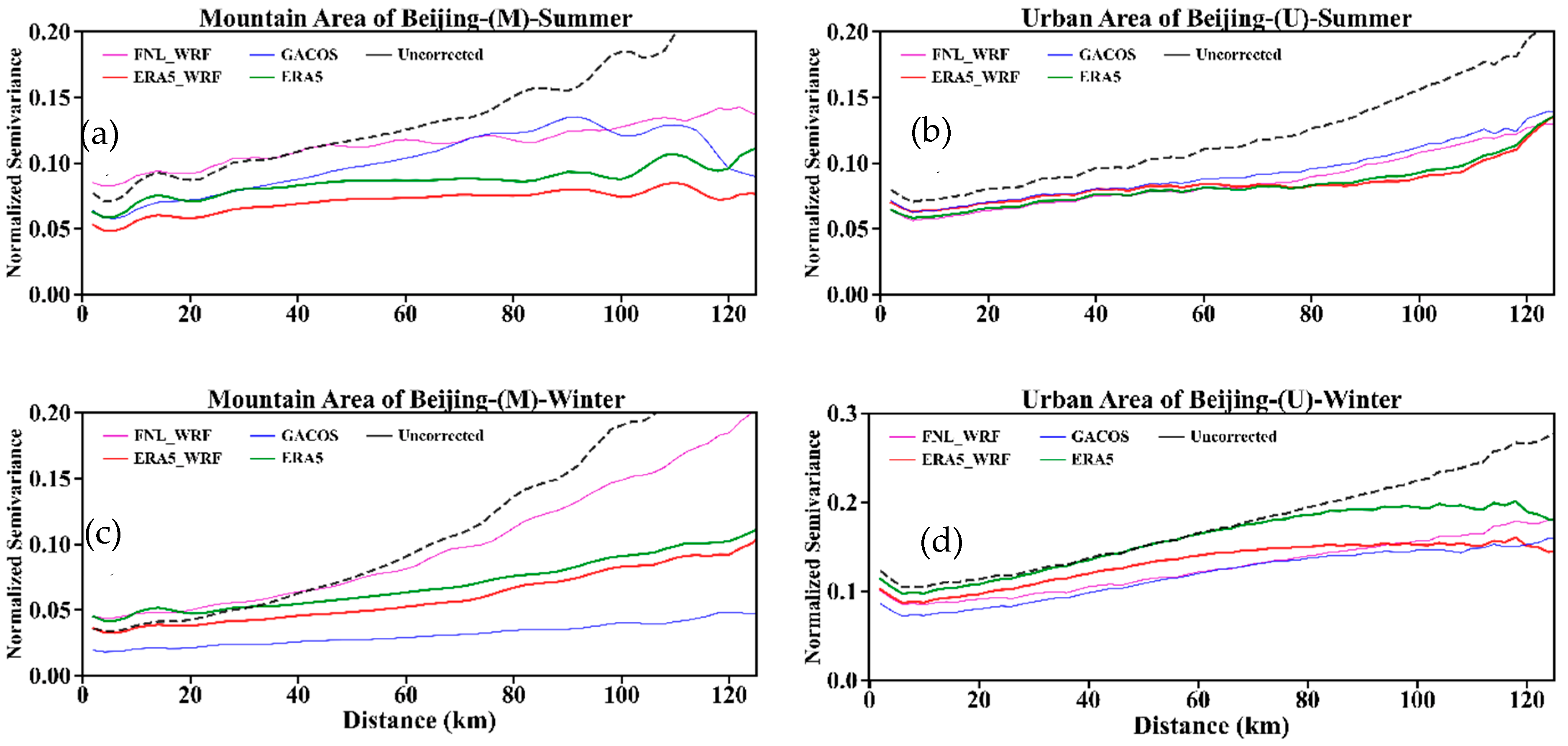
- Semi-variograms
- (4)
- Summary
5. Discussion and Analysis
5.1. Local Space-Typical Regions with Different Tropospheric Conditions
- (1)
- Beijing
- (2)
- Taiwan
5.2. Time-Seasonality Effects
5.3. Effect of Duration of Simulation on Correction by ERA5_WRF
6. Conclusions
- Regarding the benefits of the 1 h resolution of data sources, ERA5_WRF performed better in the case of large hourly variation.
- Effective simulation of WRF contributed to better performance of ERA5_WRF in terms of the corrective effects in interferograms with a large content of tropospheric delay, both for the elevation-dependent delay and spatially correlated delay.
- In areas with a highly complex topography, users need to consider the balance between improvement in accuracy and the complexity of the correction when using ERA5_WRF.
Supplementary Materials
Author Contributions
Funding
Acknowledgments
Conflicts of Interest
References
- Cao, Y.; Jónsson, S.; Li, Z. Advanced InSAR Tropospheric Corrections from Global Atmospheric Models that Incorporate Spatial Stochastic Properties of the Troposphere. J. Geophys. Res. Solid Earth 2021, 126, e2020JB020952. [Google Scholar] [CrossRef]
- Parker, A.L.; Biggs, J.; Walters, R.J.; Ebmeier, S.K.; Wright, T.J.; Teanby, N.A.; Lu, Z. Systematic assessment of atmospheric uncertainties for InSAR data at volcanic arcs using large-scale atmospheric models: Application to the Cascade volcanoes, United States. Remote Sens. Environ. 2015, 170, 102–114. [Google Scholar] [CrossRef] [Green Version]
- Dong, J.; Zhang, L.; Liao, M.; Gong, J. Improved correction of seasonal tropospheric delay in InSAR observations for landslide deformation monitoring. Remote Sens. Environ. 2019, 233, 111370. [Google Scholar] [CrossRef]
- Yu, C.; Li, Z.; Penna, N.T. Triggered afterslip on the southern Hikurangi subduction interface following the 2016 Kaikōura earthquake from InSAR time series with atmospheric corrections. Remote Sens. Environ. 2020, 251, 112097. [Google Scholar] [CrossRef]
- Hanssen, R.F.; SpringerLink. Radar Interferometry: Data Interpretation and Error Analysis; Kluwer Academic Publishers: Hingham, MA, USA, 2001; Volume 2. [Google Scholar]
- Murray, K.D.; Bekaert, D.P.; Lohman, R.B. Tropospheric corrections for InSAR: Statistical assessments and applications to the Central United States and Mexico. Remote Sens. Environ. 2019, 232, 111326. [Google Scholar] [CrossRef]
- Jung, J.; Kim, D.-J.; Park, S.-E. Correction of Atmospheric Phase Screen in Time Series InSAR Using WRF Model for Monitoring Volcanic Activities. IEEE Trans. Geosci. Remote Sens. 2014, 52, 2678–2689. [Google Scholar] [CrossRef]
- Albino, F.; Biggs, J.; Yu, C.; Li, Z. Automated Methods for Detecting Volcanic Deformation Using Sentinel-1 InSAR Time Series Illustrated by the 2017–2018 Unrest at Agung, Indonesia. J. Geophys. Res. Solid Earth 2020, 125, e2019JB017908. [Google Scholar] [CrossRef] [Green Version]
- Zebker, H.A.; Rosen, P.A.; Hensley, S. Atmospheric effects in interferometric synthetic aperture radar surface deformation and topographic maps. J. Geophys. Res. Solid Earth 1997, 102, 7547–7563. [Google Scholar] [CrossRef]
- Bekaert, D.P.S.; Hooper, A.; Wright, T.J. A spatially variable power law tropospheric correction technique for InSAR data. J. Geophys. Res. Solid Earth 2015, 120, 1345–1356. [Google Scholar] [CrossRef]
- Doin, M.-P.; Lasserre, C.; Peltzer, G.; Cavalié, O.; Doubre, C. Corrections of stratified tropospheric delays in SAR interferometry: Validation with global atmospheric models. J. Appl. Geophys. 2009, 69, 35–50. [Google Scholar] [CrossRef]
- Fattahi, H.; Amelung, F. InSAR bias and uncertainty due to the systematic and stochastic tropospheric delay. J. Geophys. Res. Solid Earth 2015, 120, 8758–8773. [Google Scholar] [CrossRef] [Green Version]
- Hu, Z.; Mallorquí, J.J. An Accurate Method to Correct Atmospheric Phase Delay for InSAR with the ERA5 Global Atmospheric Model. Remote Sens. 2019, 11, 1969. [Google Scholar] [CrossRef] [Green Version]
- Kim, J.-R.; Lin, S.-Y.; Yun, H.-W.; Tsai, Y.-L.; Seo, H.-J.; Hong, S.; Choi, Y. Investigation of Potential Volcanic Risk from Mt. Baekdu by DInSAR Time Series Analysis and Atmospheric Correction. Remote Sens. 2017, 9, 138. [Google Scholar] [CrossRef] [Green Version]
- Yun, Y. Mitigating Atmospheric Effects in Repeat-Pass Spaceborne InSAR Measurement through Data Assimilation and Numerical Simulations with WRF Model; Peking University: Beijing, China, 2015. [Google Scholar]
- Welch, M.D.; Schmidt, D.A. Separating volcanic deformation and atmospheric signals at Mount St. Helens using Persistent Scatterer InSAR. J. Volcanol. Geotherm. Res. 2017, 344, 52–64. [Google Scholar] [CrossRef]
- Wicks, C.W.; Dzurisin, D.; Ingebritsen, S.; Thatcher, W.; Lu, Z.; Iverson, J. Magmatic activity beneath the quiescent Three Sisters volcanic center, central Oregon Cascade Range, USA. Geophys. Res. Lett. 2002, 29, 26-1–26-4. [Google Scholar] [CrossRef] [Green Version]
- Lin, Y.-N.N.; Simons, M.; Hetland, E.A.; Muse, P.; DiCaprio, C. A multiscale approach to estimating topographically correlated propagation delays in radar interferograms. Geochem. Geophys. Geosystems 2010, 11, Q09002. [Google Scholar] [CrossRef]
- Béjar-Pizarro, M.; Socquet, A.; Armijo, R.; Carrizo, D.; Genrich, J.; Simons, M. Andean structural control on interseismic coupling in the North Chile subduction zone. Nat. Geosci. 2013, 6, 462–467. [Google Scholar] [CrossRef] [Green Version]
- Shen, L.; Hooper, A.; Elliott, J. A Spatially Varying Scaling Method for InSAR Tropospheric Corrections Using a High-Resolution Weather Model. J. Geophys. Res. Solid Earth 2019, 124, 4051–4068. [Google Scholar] [CrossRef] [Green Version]
- Massonnet, D.; Feigl, K.L. Discrimination of geophysical phenomena in satellite radar interferograms. Geophys. Res. Lett. 1995, 22, 1537–1540. [Google Scholar] [CrossRef]
- González, P.J.; Fernandez, J. Error estimation in multitemporal InSAR deformation time series, with application to Lanzarote, Canary Islands. J. Geophys. Res. Earth Surf. 2011, 116, B10404. [Google Scholar] [CrossRef]
- Cao, Y.; Li, Z.; Wei, J.; Hu, J.; Duan, M.; Feng, G. Stochastic modeling for time series InSAR: With emphasis on atmospheric effects. J. Geodesy 2018, 92, 185–204. [Google Scholar] [CrossRef]
- Li, Z.; Cao, Y.; Wei, J.; Duan, M.; Wu, L.; Hou, J.; Zhu, J. Time-series InSAR ground deformation monitoring: Atmospheric delay modeling and estimating. Earth-Sci. Rev. 2019, 192, 258–284. [Google Scholar] [CrossRef]
- Foster, J.; Kealy, J.; Cherubini, T.; Businger, S.; Lu, Z.; Murphy, M. The utility of atmospheric analyses for the mitigation of artifacts in InSAR. J. Geophys. Res. Solid Earth 2013, 118, 748–758. [Google Scholar] [CrossRef] [Green Version]
- Shamshiri, R.; Motagh, M.; Nahavandchi, H.; Haghighi, M.H.; Hoseini, M. Improving tropospheric corrections on large-scale Sentinel-1 interferograms using a machine learning approach for integration with GNSS-derived zenith total delay (ZTD). Remote Sens. Environ. 2020, 239, 111608. [Google Scholar] [CrossRef]
- Yu, C.; Li, Z.; Penna, N.T.; Crippa, P. Generic Atmospheric Correction Model for Interferometric Synthetic Aperture Radar Observations. J. Geophys. Res.-Solid Earth 2018, 123, 9202–9222. [Google Scholar] [CrossRef]
- Xiong, W.; Luo, S. InSAR Observation and Fault Rupture Study of the Jiuzhaigou M_S7.0Earthquake. J. Geod. Geodyn. 2019, 39, 452–457. [Google Scholar]
- Vaka, D.S.; Rao, Y.S.; Bhattacharya, A. Surface displacements of the 12 November 2017 Iran–Iraq earthquake derived using SAR interferometry. Geocarto Int. 2019, 36, 660–675. [Google Scholar] [CrossRef]
- Song, X.; Shan, X.; Qu, C. Interseismic strain accumulation across the zemuhe-daliangshan fault zone in heavily-vegetated southwestern China, From Alos-2 Interferometric Observation. In Proceedings of the IGARSS 2019—2019 IEEE International Geoscience and Remote Sensing Symposium, Yokohama, Japan, 28 July–2 August 2019; pp. 1490–1493. [Google Scholar]
- Mateus, P.; Nico, G.; Catalao, J. Uncertainty Assessment of the Estimated Atmospheric Delay Obtained by a Numerical Weather Model (NMW). IEEE Trans. Geosci. Remote Sens. 2015, 53, 6710–6717. [Google Scholar] [CrossRef]
- Jung, J.; Kim, D.-j. Correction of tropospheric phase delay in time series InSAR using WRF model for monitoring Shinmoedake volcano. In Proceedings of the 2013 IEEE International Geoscience and Remote Sensing Symposium, IEEE International Symposium on Geoscience and Remote Sensing IGARSS, Melbourne, Australia, 21–26 July 2013; pp. 137–140. [Google Scholar]
- Mateus, P.; Nico, G.; Tome, R.; Catalao, J.; Miranda, P.M.A. Experimental Study on the Atmospheric Delay Based on GPS, SAR Interferometry, and Numerical Weather Model Data. IEEE Trans. Geosci. Remote Sens. 2013, 51, 6–11. [Google Scholar] [CrossRef]
- Zhang, Z.; Lou, Y.; Zhang, W.; Wang, H.; Zhou, Y.; Bai, J. On the Assessment GPS-Based WRFDA for InSAR Atmospheric Correction: A Case Study in Pearl River Delta Region of China. Remote Sens. 2021, 13, 3280. [Google Scholar] [CrossRef]
- Yun, Y.; Zeng, Q.; Green, B.W.; Zhang, F. Mitigating atmospheric effects in InSAR measurements through high-resolution data assimilation and numerical simulations with a weather prediction model. Int. J. Remote Sens. 2015, 36, 2129–2147. [Google Scholar] [CrossRef]
- Miranda, P.M.A.; Mateus, P.; Nico, G.; Catalão, J.; Tomé, R.; Nogueira, M. InSAR Meteorology: High-Resolution Geodetic Data Can Increase Atmospheric Predictability. Geophys. Res. Lett. 2019, 46, 2949–2955. [Google Scholar] [CrossRef] [Green Version]
- Mateus, P.; Miranda, P.M.A.; Nico, G.; Catalao, J. Continuous Multitrack Assimilation of Sentinel-1 Precipitable Water Vapor Maps for Numerical Weather Prediction: How Far Can We Go with Current InSAR Data? J. Geophys. Res. Atmos. 2021, 126, e2020JD034171. [Google Scholar] [CrossRef]
- Mateus, P.; Miranda, P.M.A. Using InSAR Data to Improve the Water Vapor Distribution Downstream of the Core of the South American Low-Level Jet. J. Geophys. Res. Atmos. 2022, 127, e2021JD036111. [Google Scholar] [CrossRef]
- Roukounakis, N.; Katsanos, D.; Briole, P.; Elias, P.; Kioutsioukis, I.; Argiriou, A.; Retalis, A. Use of GNSS Tropospheric Delay Measurements for the Parameterization and Validation of WRF High-Resolution Re-Analysis over the Western Gulf of Corinth, Greece: The PaTrop Experiment. Remote Sens. 2021, 13, 1898. [Google Scholar] [CrossRef]
- Wang, X.; Zeng, Q.; Jiao, J.; Hao, Z. Evaluation of Weather Research and Forecast (WRF) microphysics schemes in simulating zenith total delay for InSAR atmospheric correction. Int. J. Remote Sens. 2021, 42, 3456–3473. [Google Scholar] [CrossRef]
- Dou, F.; Lv, X.; Chai, H. Mitigating Atmospheric Effects in InSAR Stacking Based on Ensemble Forecasting with a Numerical Weather Prediction Model. Remote Sens. 2021, 13, 4670. [Google Scholar] [CrossRef]
- Ulmer, F.-G.; Adam, N. Characterisation and improvement of the structure function estimation for application in PSI. ISPRS J. Photogramm. Remote Sens. 2017, 128, 40–46. [Google Scholar] [CrossRef] [Green Version]
- Adam, N. Methodology of a Troposphere Effect Mitigation Processor for SAR Interferometry. IEEE J. Sel. Top. Appl. Earth Obs. Remote Sens. 2019, 12, 5334–5344. [Google Scholar] [CrossRef]
- Zeng, Q.; Zhang, X.; Jiao, J. Atmospheric correction of spaceborne repeat-pass InSAR DEM generation based on WRF. J. Remote Sens. 2016, 20, 1151–1160. [Google Scholar]
- Wang, X.; Zeng, Q.; Yun, Y.; Han, K.; Jiao, J. The reliability inspection of water vapor from WRF utilized for InSAR atmospheric correction in different areas. In Proceedings of the 2017 IEEE International Geoscience and Remote Sensing Symposium, IEEE International Symposium on Geoscience and Remote Sensing IGARSS, Fort Worth, TX, USA, 23–28 July 2017; pp. 3105–3108. [Google Scholar]
- Kinoshita, Y.; Furuya, M.; Hobiger, T.; Ichikawa, R. Are numerical weather model outputs helpful to reduce tropospheric delay signals in InSAR data? J. Geod. 2013, 87, 267–277. [Google Scholar] [CrossRef] [Green Version]
- Roukounakis, N.; Elias, P.; Briole, P.; Katsanos, D.; Kioutsioukis, I.; Argiriou, A.; Retalis, A. Tropospheric Correction of Sentinel-1 Synthetic Aperture Radar Interferograms Using a High-Resolution Weather Model Validated by GNSS Measurements. Remote Sens. 2021, 13, 2258. [Google Scholar] [CrossRef]
- Xiong, S.; Zeng, Q.; Jiao, J.; Zhang, X. PS-InSAR analysis for Radarsat-2 datasets in Guangdong Province to detect accurate land deformation. Dragon 3Mid Term Results 2014, 724, 111. [Google Scholar]
- Darvishi, M.; Cuozzo, G.; Bruzzone, L.; Nilfouroushan, F. Performance Evaluation of Phase and Weather-Based Models in Atmospheric Correction with Sentinel-1Data: Corvara Landslide in the Alps. IEEE J. Sel. Top. Appl. Earth Obs. Remote Sens. 2020, 13, 1332–1346. [Google Scholar] [CrossRef]
- Gong, W.; Meyer, F.J.; Liu, S.; Hanssen, R.F. Temporal Filtering of InSAR Data Using Statistical Parameters from NWP Models. IEEE Trans. Geosci. Remote Sens. 2015, 53, 4033–4044. [Google Scholar] [CrossRef]
- Yun, Y.; Zeng, Q.; Lv, X. Understanding Mountain-Wave Phases in ERS Tandem DInSAR Interferogram Using WRF Model Simulation. IEEE Trans. Geosci. Remote Sens. 2018, 56, 2762–2771. [Google Scholar] [CrossRef]
- Yu, C.; Li, Z.; Chen, J.; Hu, J.-C. Small Magnitude Co-Seismic Deformation of the 2017 Mw 6.4 Nyingchi Earthquake Revealed by InSAR Measurements with Atmospheric Correction. Remote Sens. 2018, 10, 684. [Google Scholar] [CrossRef] [Green Version]
- Chen, B.; Gong, H.; Chen, Y.; Lei, K.; Zhou, C.; Si, Y.; Li, X.; Pan, Y.; Gao, M. Investigating land subsidence and its causes along Beijing high-speed railway using multi-platform InSAR and a maximum entropy model. Int. J. Appl. Earth Obs. Geoinf. 2021, 96, 102284. [Google Scholar] [CrossRef]
- Navarro-Hernández, M.; Tomás, R.; Lopez-Sanchez, J.; Cárdenas-Tristán, A.; Mallorquí, J. Spatial Analysis of Land Subsidence in the San Luis Potosi Valley Induced by Aquifer Overexploitation Using the Coherent Pixels Technique (CPT) and Sentinel-1 InSAR Observation. Remote Sens. 2020, 12, 3822. [Google Scholar] [CrossRef]
- Hu, L.; Dai, K.; Xing, C.; Li, Z.; Tomás, R.; Clark, B.; Shi, X.; Chen, M.; Zhang, R.; Qiu, Q.; et al. Land subsidence in Beijing and its relationship with geological faults revealed by Sentinel-1 InSAR observations. Int. J. Appl. Earth Obs. Geoinf. 2019, 82, 101886. [Google Scholar] [CrossRef]
- Xu, H.; Luo, Y.; Yang, B.; Li, Z.; Liu, W. Tropospheric Delay Correction Based on a Three-Dimensional Joint Model for InSAR. Remote Sens. 2019, 11, 2542. [Google Scholar] [CrossRef] [Green Version]
- Jian, H.; Wang, L.; Gan, W.; Zhang, K.; Li, Y.; Liang, S.; Liu, Y.; Gong, W.; Yin, X. Geodetic Model of the 2017 Mw 6.5 Mainling Earthquake Inferred from GPS and InSAR Data. Remote Sens. 2019, 11, 2940. [Google Scholar] [CrossRef] [Green Version]
- Maroufpoor, S.; Bozorg-Haddad, O.; Chu, X. Chapter 9—Geostatistics: Principles and methods. In Handbook of Probabilistic Models; Samui, P., Tien Bui, D., Chakraborty, S., Deo, R.C., Eds.; Butterworth-Heinemann: Oxford, UK, 2020; pp. 229–242. [Google Scholar]
- Somos-Valenzuela, M.; Manquehual-Cheuque, F. Evaluating Multiple WRF Configurations and Forcing over the Northern Patagonian Icecap (NPI) and Baker River Basin. Atmosphere 2020, 11, 815. [Google Scholar] [CrossRef]
- Duzenli, E.; Yucel, I.; Pilatin, H.; Yilmaz, M.T. Evaluating the performance of a WRF initial and physics ensemble over Eastern Black Sea and Mediterranean regions in Turkey. Atmos. Res. 2021, 248, 105184. [Google Scholar] [CrossRef]
- Hong, S.-Y.; Dudhia, J.; Chen, S.-H. A Revised Approach to Ice Microphysical Processes for the Bulk Parameterization of Clouds and Precipitation. Mon. Weather. Rev. 2004, 132, 103–120. [Google Scholar] [CrossRef]
- Kain, J.S. The Kain–Fritsch Convective Parameterization: An Update. J. Appl. Meteorol. 2004, 43, 170–181. [Google Scholar] [CrossRef]
- Mlawer, E.J.; Taubman, S.J.; Brown, P.D.; Iacono, M.J.; Clough, S.A. Radiative transfer for inhomogeneous atmospheres: RRTM, a validated correlated-k model for the longwave. J. Geophys. Res. Atmos. 1997, 102, 16663–16682. [Google Scholar] [CrossRef] [Green Version]
- Iacono, M.J.; Delamere, J.S.; Mlawer, E.J.; Shephard, M.W.; Clough, S.A.; Collins, W.D. Radiative forcing by long-lived greenhouse gases: Calculations with the AER radiative transfer models. J. Geophys. Res. Atmos. 2008, 113, D13103. [Google Scholar] [CrossRef]
- Niu, G.-Y.; Yang, Z.-L.; Mitchell, K.E.; Chen, F.; Ek, M.B.; Barlage, M.; Kumar, A.; Manning, K.; Niyogi, D.; Rosero, E.; et al. The community Noah land surface model with multiparameterization options (Noah-MP): 1. Model description and evaluation with local-scale measurements. J. Geophys. Res. Atmos. 2011, 116, D12109. [Google Scholar] [CrossRef] [Green Version]
- Hong, S.-Y.; Noh, Y.; Dudhia, J. A New Vertical Diffusion Package with an Explicit Treatment of Entrainment Processes. Mon. Weather. Rev. 2006, 134, 2318–2341. [Google Scholar] [CrossRef] [Green Version]
- Jiménez, P.A.; Dudhia, J.; González-Rouco, J.F.; Navarro, J.; Montávez, J.P.; García-Bustamante, E. A Revised Scheme for the WRF Surface Layer Formulation. Mon. Weather. Rev. 2012, 140, 898–918. [Google Scholar] [CrossRef] [Green Version]
- Skamarock, W.C.; Klemp, J.B.; Dudhia, J.; Gill, D.O.; Liu, Z.; Berner, J.; Wang, W.; Powers, J.G.; Duda, M.G.; Barker, D.M.; et al. A Description of the Advanced Research WRF Version 4; National Center for Atmospheric Research: Boulder, CO, USA, 2019. [Google Scholar]
- Liang, X.; Li, Q.; Mei, H.; Zeng, M. Multi-Grid Nesting Ability to Represent Convections Across the Gray Zone. J. Adv. Model. Earth Syst. 2019, 11, 4352–4376. [Google Scholar] [CrossRef]


| SAR Image Acquisition Date and UTC Time | |||
|---|---|---|---|
| Cases | Beijing | Taiwan | Nyingchi |
| Master Image | 5 July 2010 02:32 | 18 July 2019 21:52 | 6 November 2017 23:42 |
| Slave Image | 13 September 2010 02:32 | 30 July 2019 21:52 | 18 November 2017 23:42 |
| SAR Image Acquisition Date | ||||||
|---|---|---|---|---|---|---|
| 10 January 2019 | 11 March 2019 | 28 April 2019 | 15 June 2019 | 2 August 2019 | 1 January 2019 | 18 November 2019 |
| 22 January 2019 | 23 March 2019 | 10 May 2019 | 27 June 2019 | 14 August 2019 | 13 October 2019 | 30 November 2019 |
| 3 February 2019 | 4 April 2019 | 22 May 2019 | 9 July 2019 | 26 August 2019 | 25 October 2019 | 12 December 2019 |
| 27 February 2019 | 16 April 2019 | 3 June 2019 | 21 July 2019 | 19 September 2019 | 6 November 2019 | 24 December 2019 |
| Parameter | Scheme |
|---|---|
| Microphysics | WSM3 [61] |
| Cumulus 1 | KF [62] |
| Long/short radiation | RRTM [63]/RRTMG [64] |
| Land surface model | Noah MP [65] |
| Planetary boundary physics | YSU [66] |
| Surface layer physics | MM5 [67] |
| Method | Data Sources | Downscaling | |||
|---|---|---|---|---|---|
| Data | Resolution | Space (Downscaling to 1 km) | Time | ||
| Space | Time | ||||
| FNL_WRF | FNL | 1° | 6 h | WRF simulation driven by two closet data | |
| ERA5_WRF | ERA5 | 0.25° | 1 h | ||
| ERA5 | Interpolation related to the position in space (especially for elevation) | Using closet data | |||
| GACOS | HRES ECMWF | 0.125° | 6 h | Iterative Tropospheric Decomposition (ITD) model | Linear temporal interpolation using two closet data |
| FNL-WRF | ERA5-WRF | ERA5 | GACOS | |
|---|---|---|---|---|
| (A) | 25.03 | 25.45 | 24.92 | 24.83 |
| (B) | 21.84 | 22.78 | 18.94 | 33.09 |
| (C) | 24.07 | 28.95 | 27.09 | 27.29 |
| (A) | −7.31 | −7.97 | −11.88 | −13.30 |
| (B) | −13.64 | −15.24 | −20.32 | −8.13 |
| (C) | −9.86 | −11.20 | −10.48 | −16.00 |
Disclaimer/Publisher’s Note: The statements, opinions and data contained in all publications are solely those of the individual author(s) and contributor(s) and not of MDPI and/or the editor(s). MDPI and/or the editor(s) disclaim responsibility for any injury to people or property resulting from any ideas, methods, instructions or products referred to in the content. |
© 2023 by the authors. Licensee MDPI, Basel, Switzerland. This article is an open access article distributed under the terms and conditions of the Creative Commons Attribution (CC BY) license (https://creativecommons.org/licenses/by/4.0/).
Share and Cite
Liu, Q.; Zeng, Q.; Zhang, Z. Evaluation of InSAR Tropospheric Correction by Using Efficient WRF Simulation with ERA5 for Initialization. Remote Sens. 2023, 15, 273. https://doi.org/10.3390/rs15010273
Liu Q, Zeng Q, Zhang Z. Evaluation of InSAR Tropospheric Correction by Using Efficient WRF Simulation with ERA5 for Initialization. Remote Sensing. 2023; 15(1):273. https://doi.org/10.3390/rs15010273
Chicago/Turabian StyleLiu, Qinghua, Qiming Zeng, and Zhiliang Zhang. 2023. "Evaluation of InSAR Tropospheric Correction by Using Efficient WRF Simulation with ERA5 for Initialization" Remote Sensing 15, no. 1: 273. https://doi.org/10.3390/rs15010273