Author Contributions
Conceptualization, H.H.; methodology, S.S.; software, Y.J. (Yigao Jin); validation, Y.Z. and J.C.; investigation, X.Y.; resources, Y.J. (Ying Jiang); data curation, Y.D. and X.G. (Xiaocui Guo); writing—original draft, S.S.; writing—review and editing, H.H.; visualization, X.G. (Xuming Ge). All authors have read and agreed to the published version of the manuscript.
Figure 1.
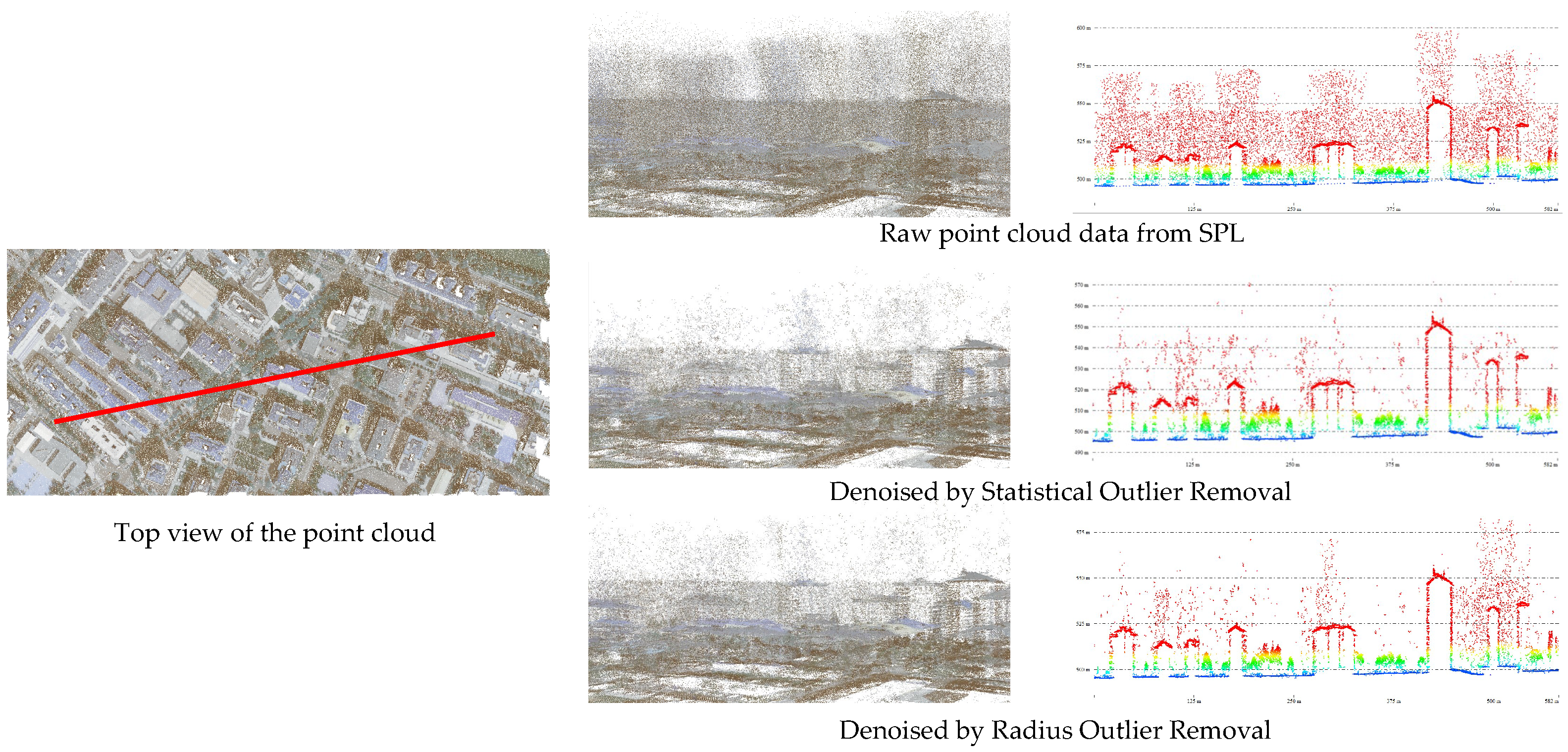
The raw point clouds data from SPL and the denoising results using existing algorithms. The three images in the right hand show the profile line in the area of the red line on the left.
Figure 1.
The raw point clouds data from SPL and the denoising results using existing algorithms. The three images in the right hand show the profile line in the area of the red line on the left.
Figure 2.
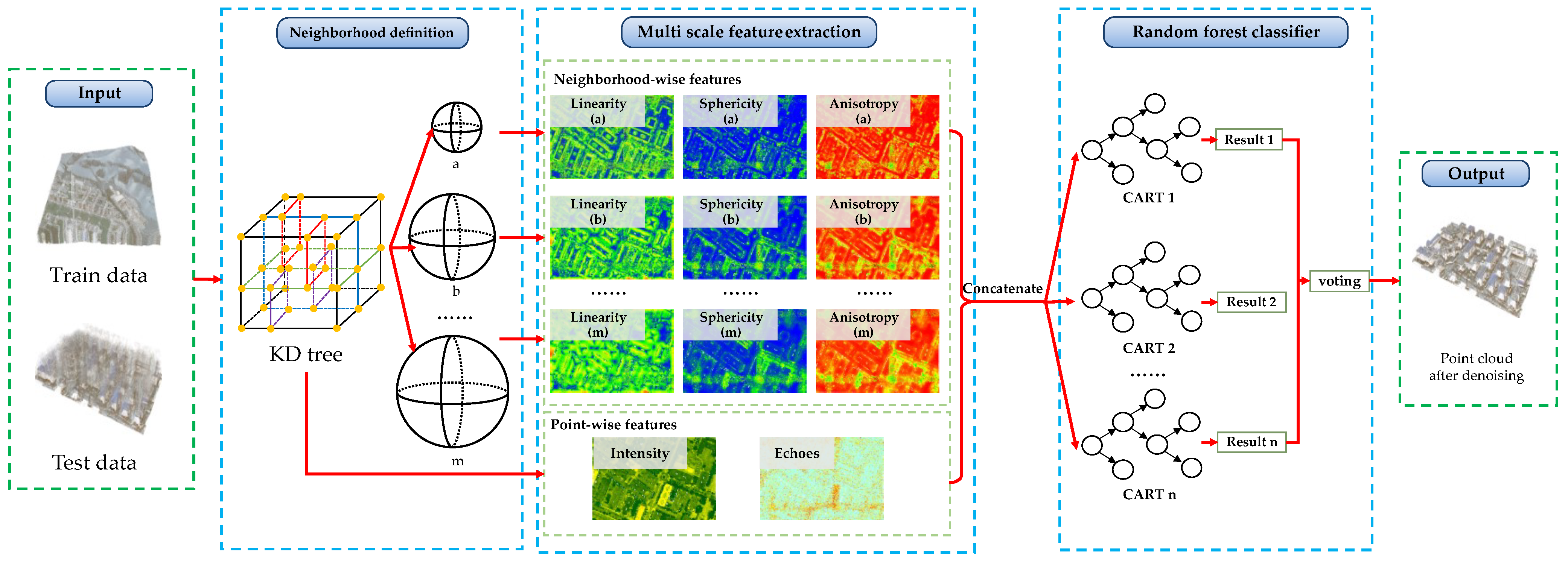
Structure of the proposed network. There are three main parts: neighborhood definition, a multiscale feature extraction, and a random forests module. In the neighborhood definition module, a,b…m represent different scales.
Figure 2.
Structure of the proposed network. There are three main parts: neighborhood definition, a multiscale feature extraction, and a random forests module. In the neighborhood definition module, a,b…m represent different scales.
Figure 3.
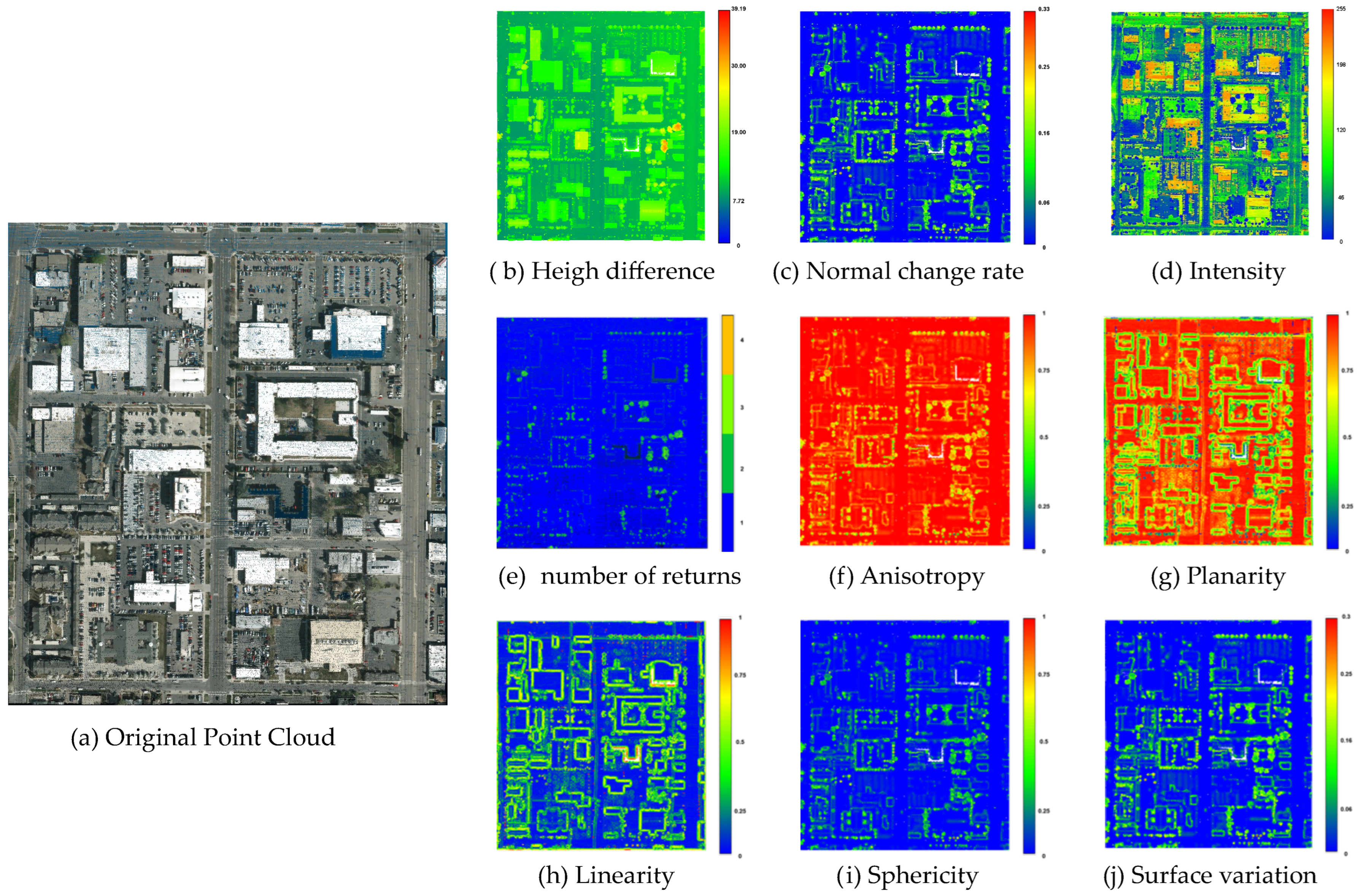
Original point cloud and some representative LiDAR point cloud features.
Figure 3.
Original point cloud and some representative LiDAR point cloud features.
Figure 4.
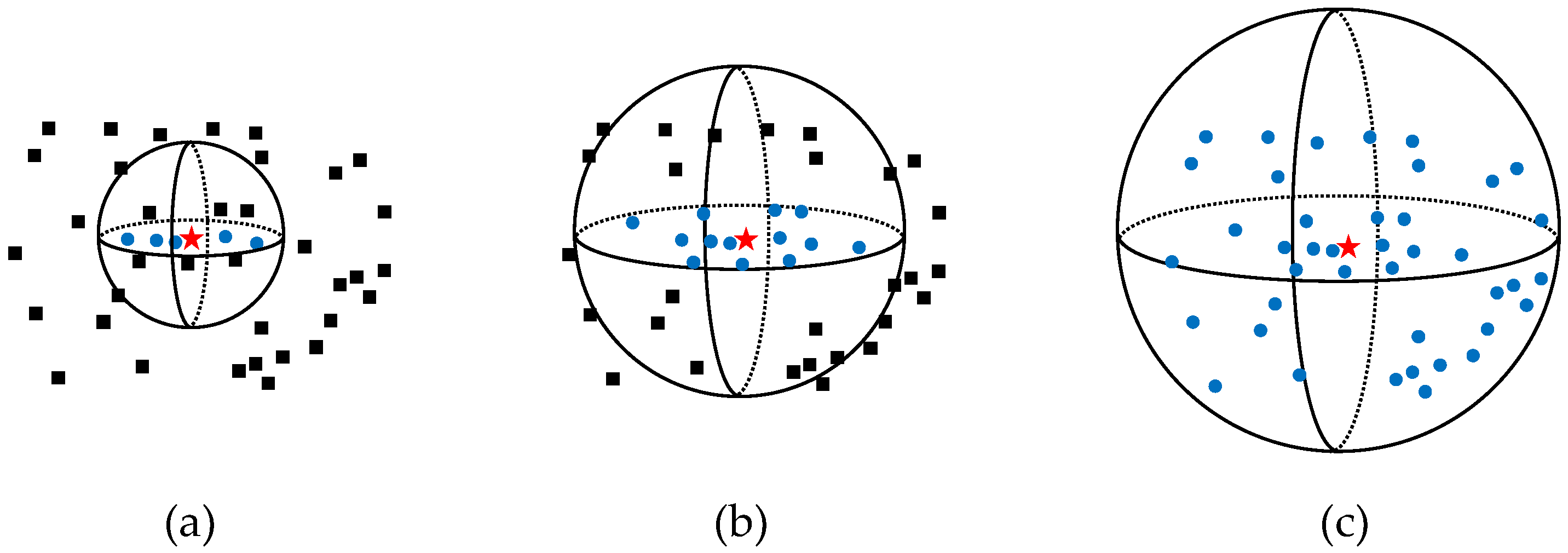
Neighborhoods at different scales. In this representation, the red star is the centroid point of the neighborhood, the blue points are the neighbors within the local neighborhood, and the black points are the outside points of the local neighborhood. In the figure, (a–c) represent different scales.
Figure 4.
Neighborhoods at different scales. In this representation, the red star is the centroid point of the neighborhood, the blue points are the neighbors within the local neighborhood, and the black points are the outside points of the local neighborhood. In the figure, (a–c) represent different scales.
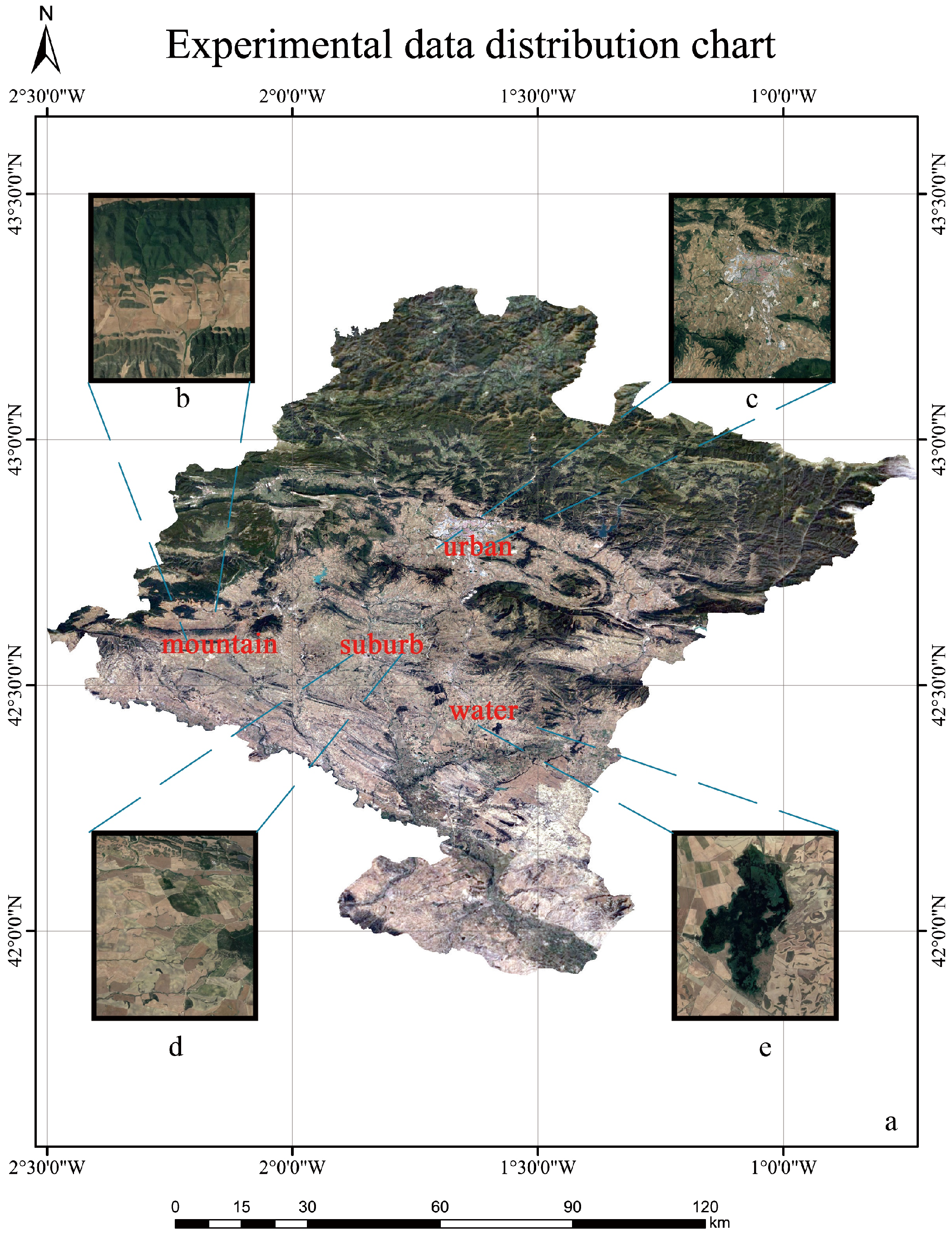
Figure 5.
Experimental data distribution chart; (a) overview map of Navarra, background: Google Earth; (b) the mountain area of Sorlada; (c) part of the urban area of Pamplona; (d) part of the suburb area of Berbinzana; (e) Laguna de Pitillas Lake and its vicinity.
Figure 5.
Experimental data distribution chart; (a) overview map of Navarra, background: Google Earth; (b) the mountain area of Sorlada; (c) part of the urban area of Pamplona; (d) part of the suburb area of Berbinzana; (e) Laguna de Pitillas Lake and its vicinity.
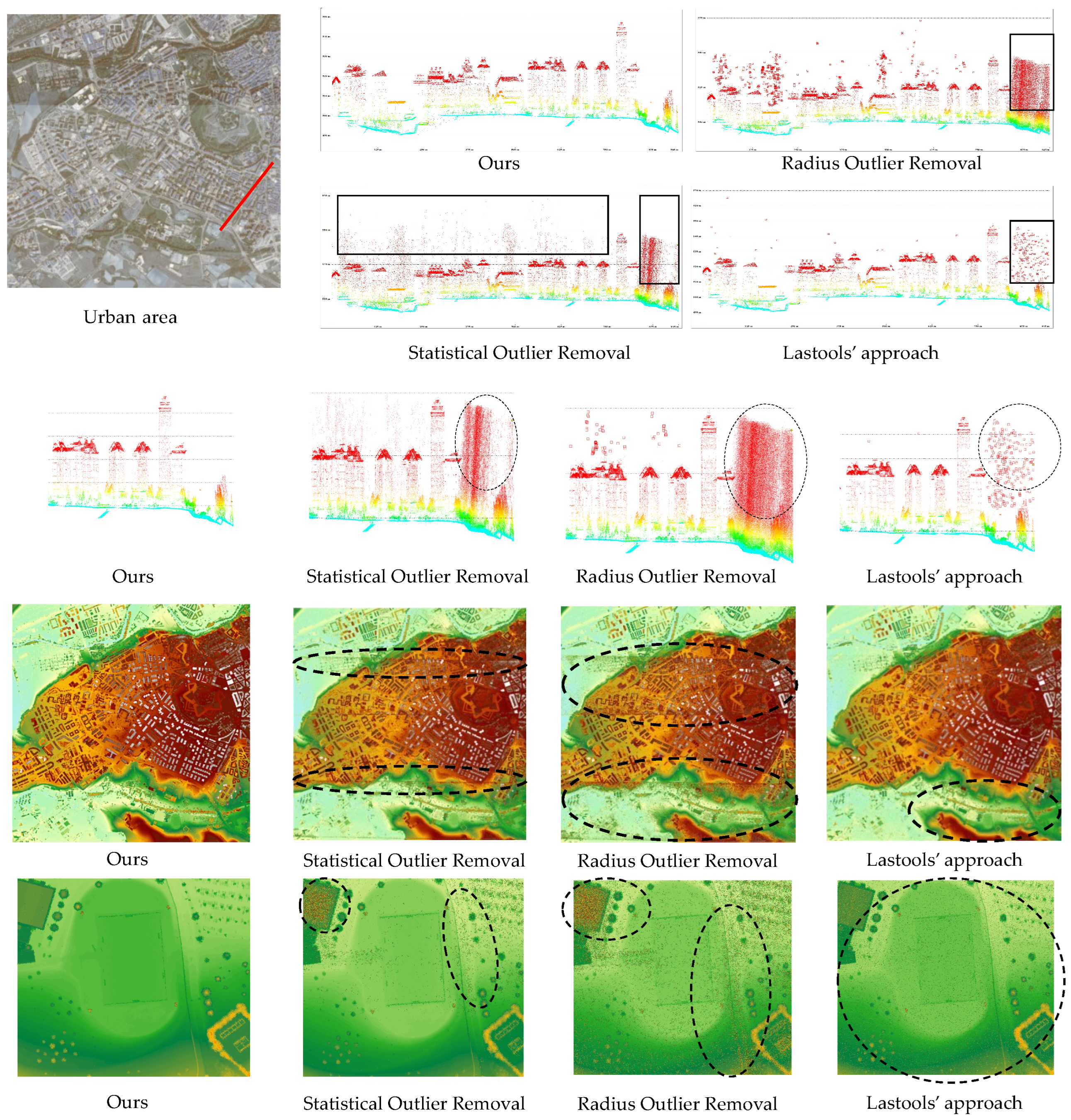
Figure 6.
Examples of the denoising results in the urban area. The four images in the upper right-hand corner show the profile line in the area of the red line on the left. The third row represents the profile line partial details for convenient comparison. The fourth row indicates the DSM generated by the different denoising methods. The bottom row indicates some details of the DSM to facilitate comparison.
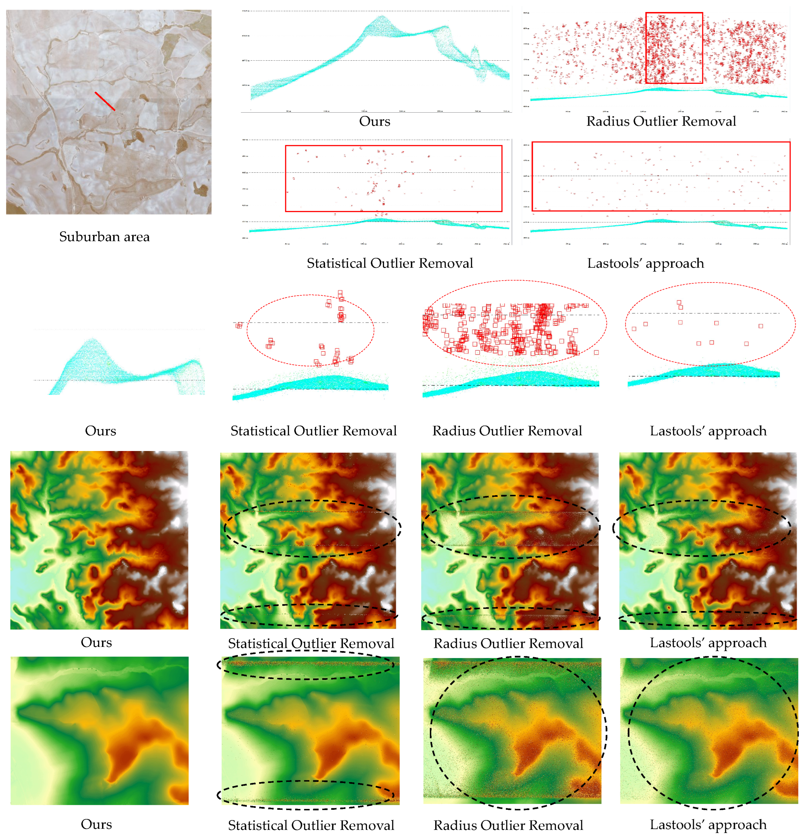
Figure 7.
Examples of the denoising results in the suburban area. The four images in the upper right-hand corner show the profile line in the area of the red line on the left. The third row represents the profile line partial details for convenient comparison. The fourth row indicates the DSM generated by the different denoising methods. The bottom row indicates some details of the DSM to facilitate comparison.
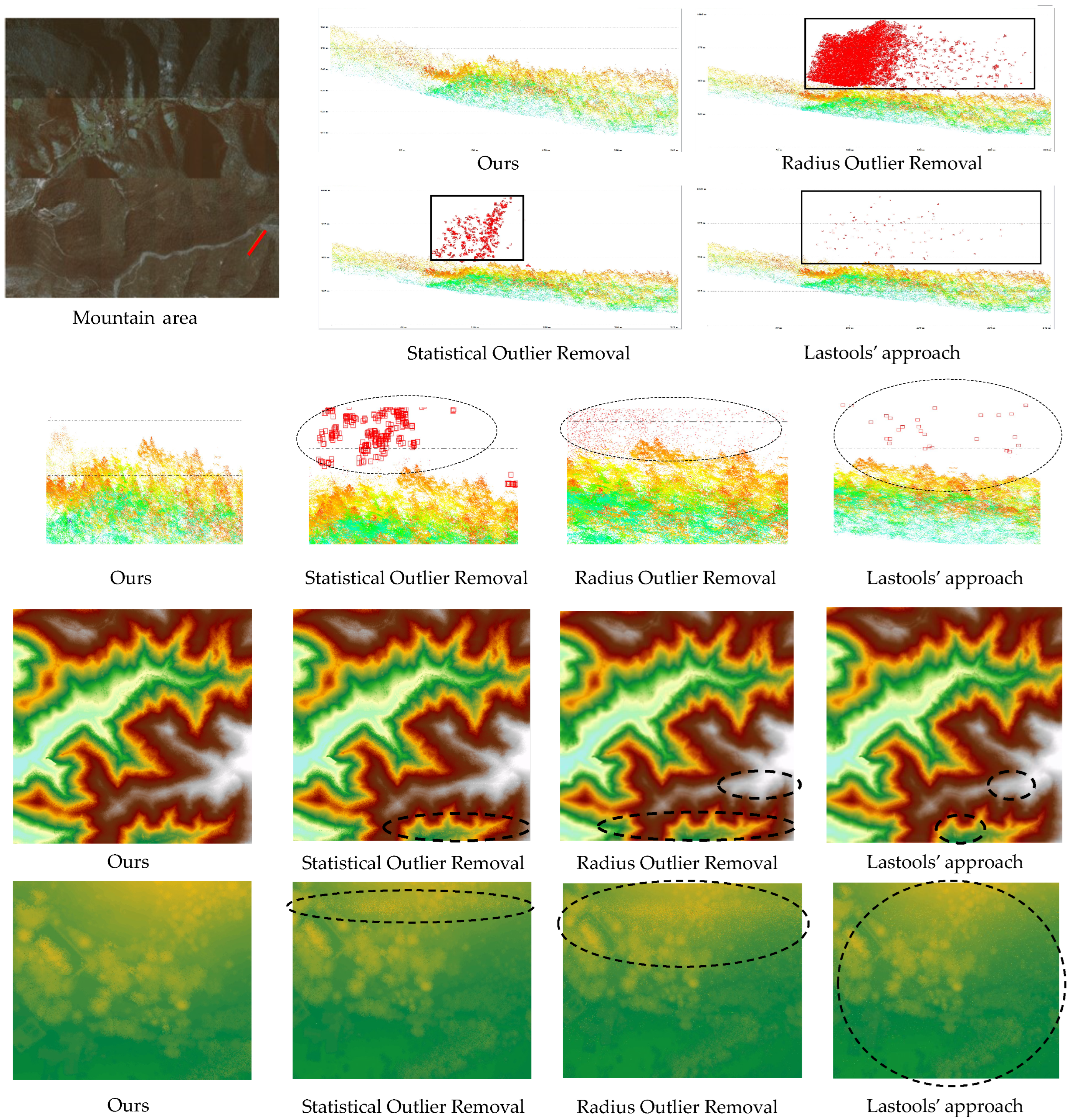
Figure 8.
Examples of the denoising results in the mountain area. The four images in the upper right-hand corner show the profile line in the area of the red line on the left. The third row represents the profile line partial details for convenient comparison. The fourth row indicates the DSM generated by the different denoising methods. The bottom row indicates some details of the DSM to facilitate comparison.
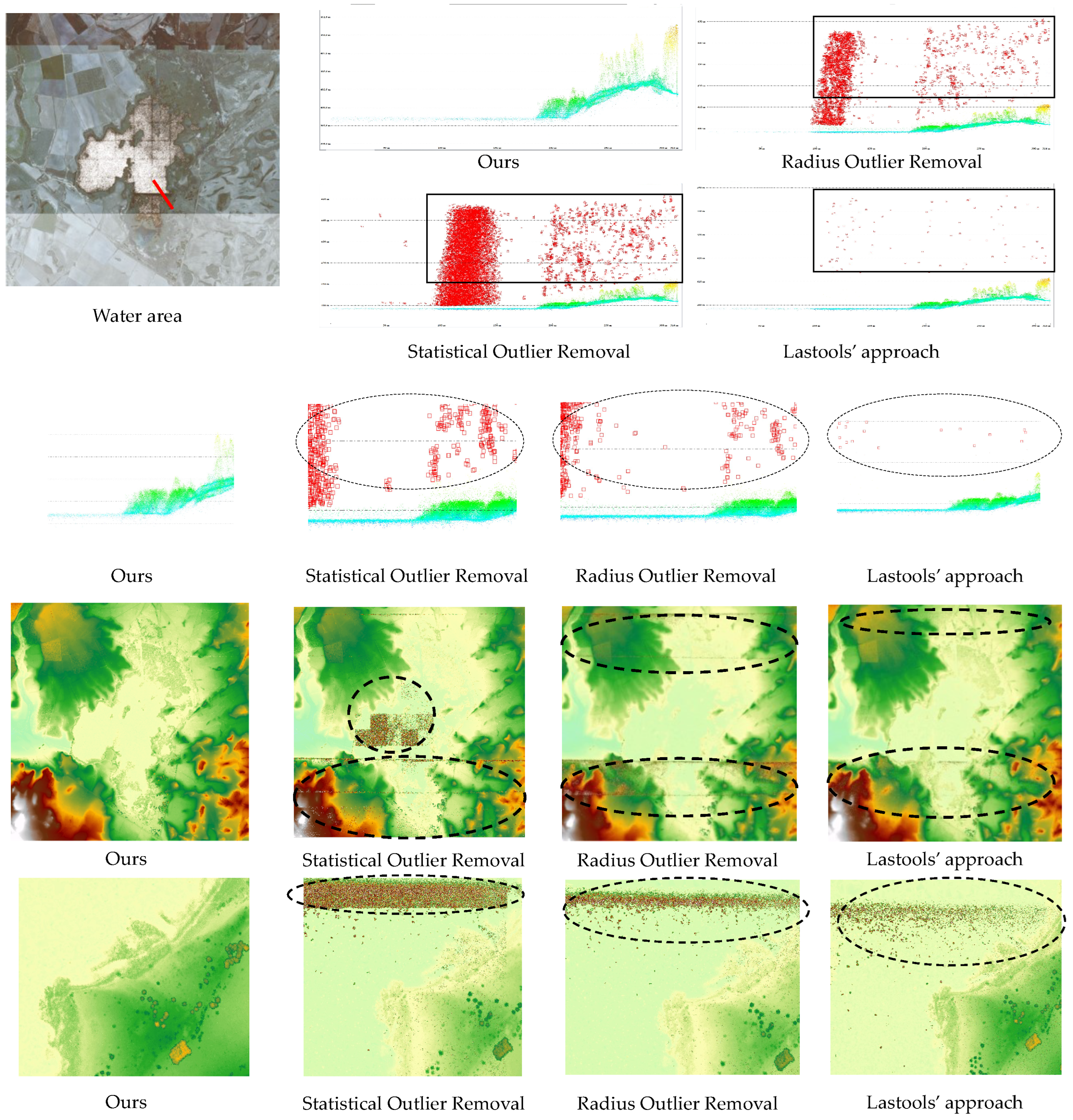
Figure 9.
Examples of the denoising results in the water area. The four images in the upper right-hand corner show the profile line in the area of the red line on the left. The third row represents the profile line partial details for convenient comparison. The fourth row indicates the DSM generated by the different denoising methods. The bottom row indicates some details of the DSM to facilitate comparison.
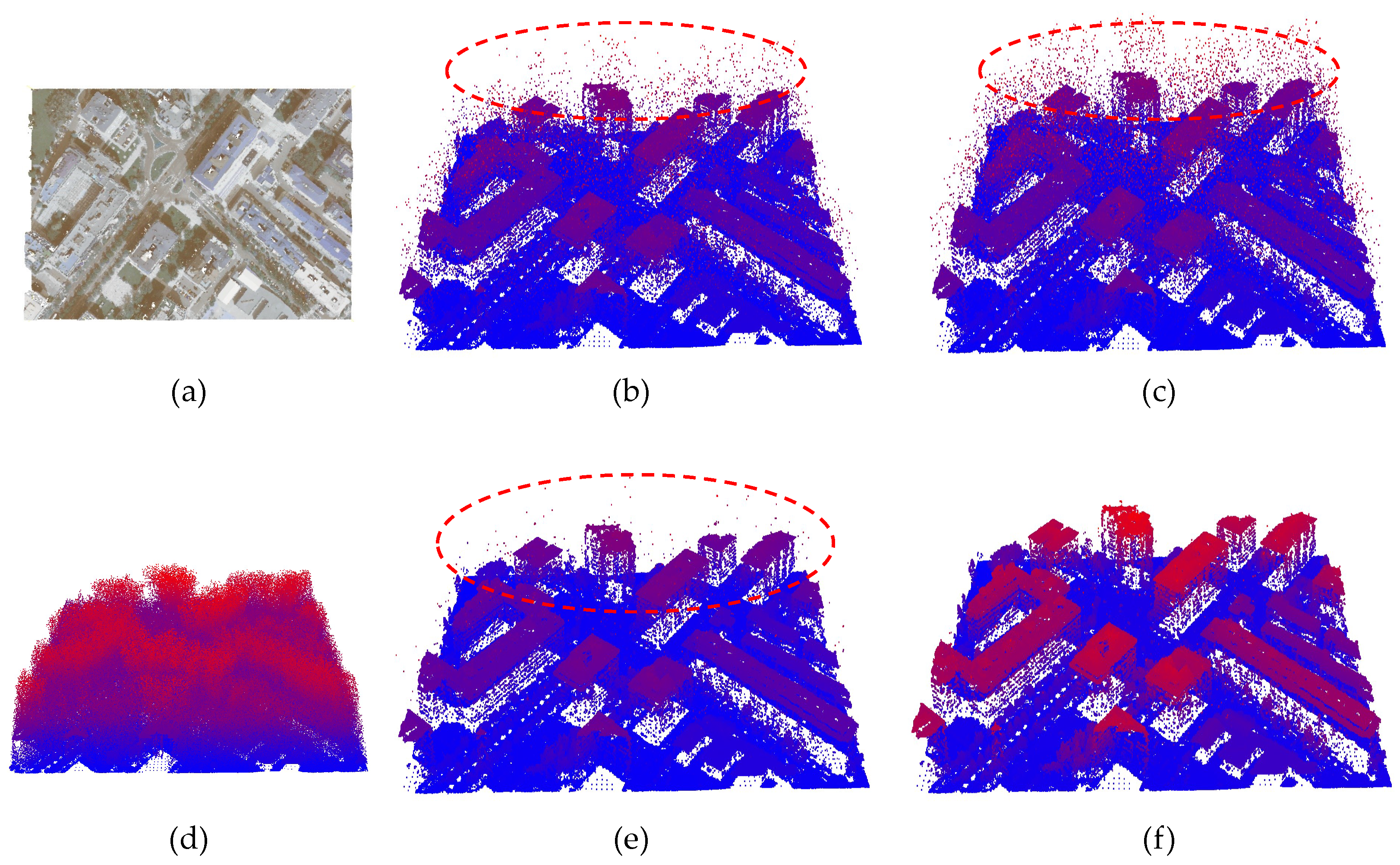
Figure 10.
Analysis of single-scale and multiscale denoising results; (a) overview of the urban area; (b) three-dimensional view after denoising in the 5 m neighborhood; (c) three-dimensional view after denoising in the 10 m neighborhood; (d) raw SPL point cloud with noise; (e) three-dimensional view after denoising in the 5 m and 10 m neighborhoods; (f) three-dimensional view after denoising in the 5 m, 10 m, and 15 m neighborhoods.
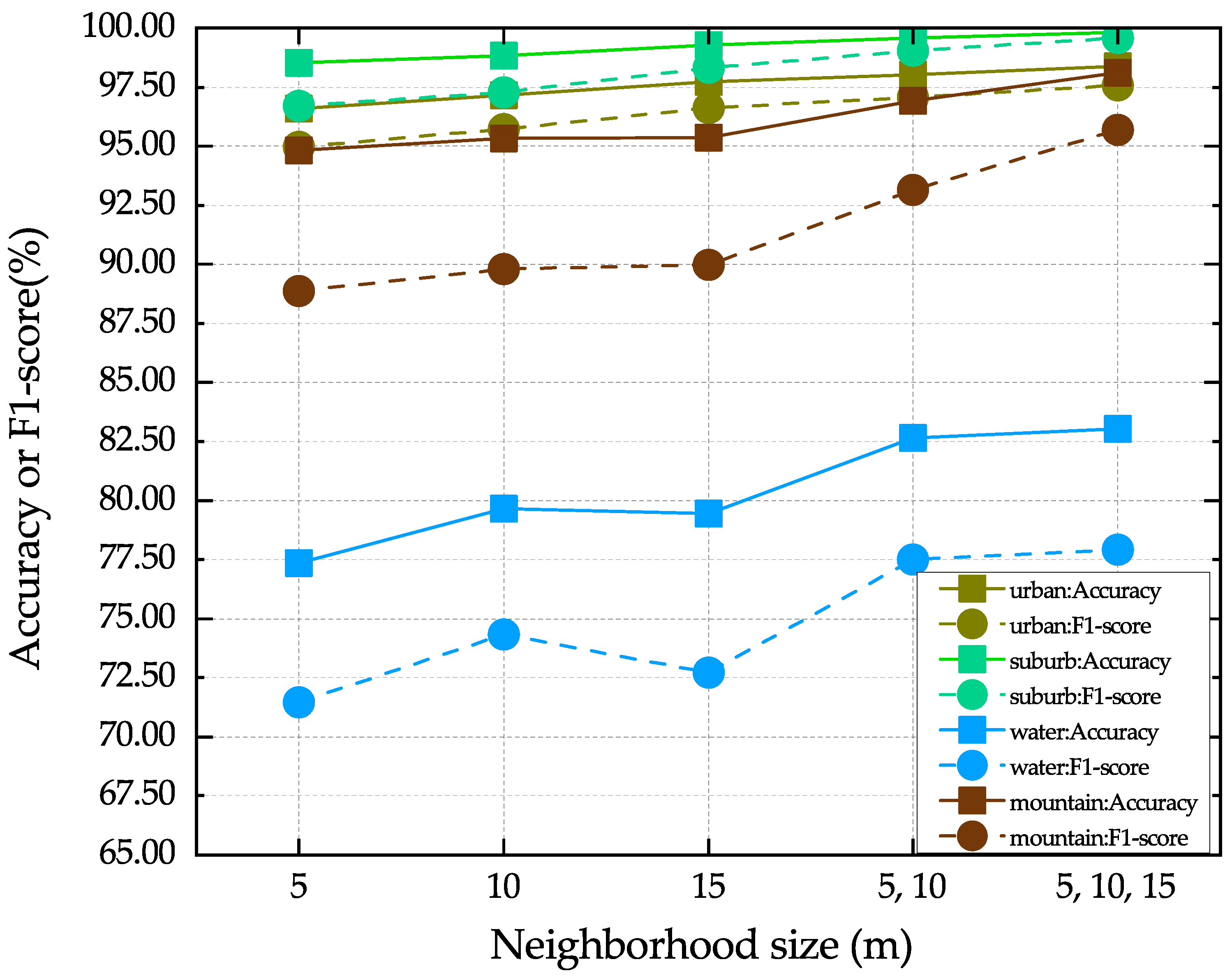
Figure 11.
Visualization of the effect of single-scale versus multiscale neighborhood features on denoising results on the four datasets.
Figure 11.
Visualization of the effect of single-scale versus multiscale neighborhood features on denoising results on the four datasets.
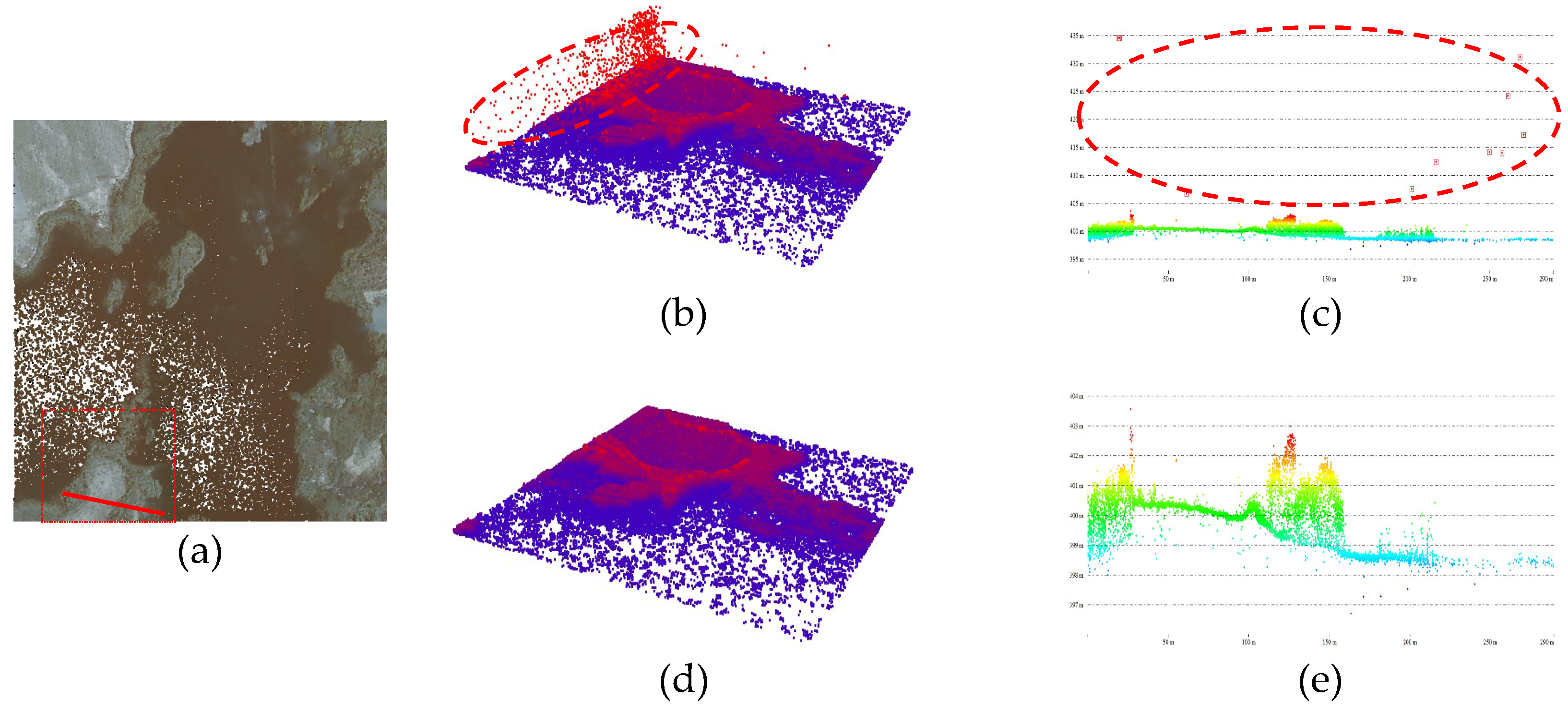
Figure 12.
Visualization of the effect of the multiple denoising in the water area using our proposed approach. (a) overview of the water area; (b) three-dimensional view after the first denoising; (c) profile after the first denoising; (d) three-dimensional view after the second denoising; (e) profile after the second denoising.
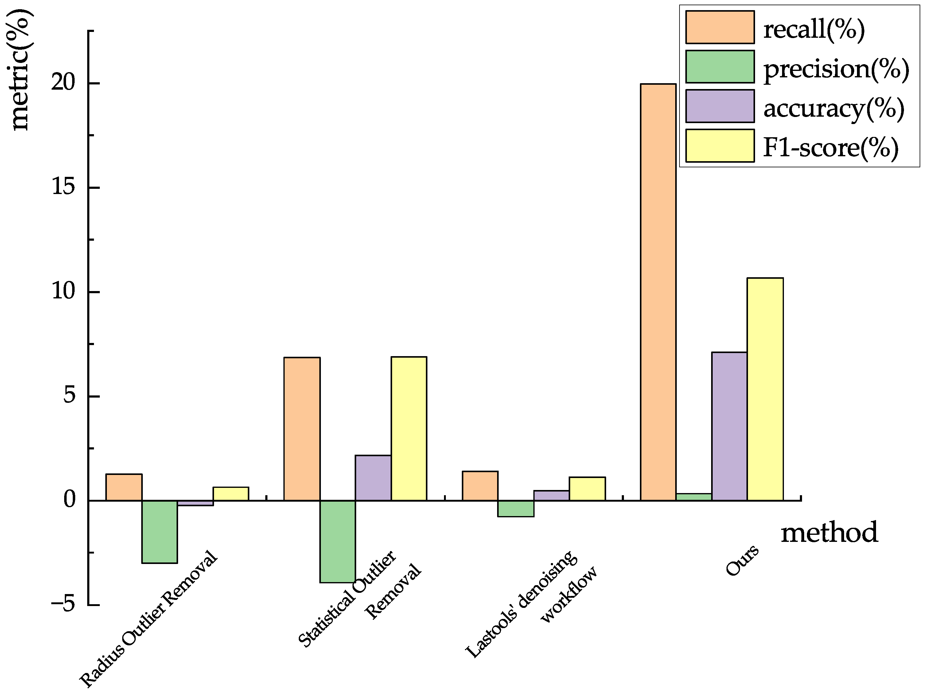
Figure 13.
Visualization of the evaluation metrics improvement after multiple denoising.
Figure 13.
Visualization of the evaluation metrics improvement after multiple denoising.
Table 1.
Dataset information.
Table 1.
Dataset information.
| Dataset Name | Navarra Dataset |
|---|
| LiDAR system | SPL100 |
| Point density | 14.5 points/m |
| Flight height | 4200 m (AGL) |
| Field of view (FoV) | 30° |
| Flight speed | 90 m/s |
| Swath width | 2260 m |
| Effective scan rate | 6 MHz |
| Data coverage | The Navarra province of Spain |
| Coordinate system | ETRS89 / UTM zone 30 N (EPSG25830) |
Table 2.
Performance evaluation of the compared approaches and ours in the urban area.
Table 2.
Performance evaluation of the compared approaches and ours in the urban area.
| Methods | Recall (%) | Precision (%) | Accuracy (%) | F1-Score (%) |
|---|
| Radius Outlier Removal | 82.63 | 98.51 | 93.71 | 89.87 |
| Statistical Outlier Removal | 65.34 | 99.55 | 88.19 | 78.89 |
| Lastools’ Denoising Workflow | 88.84 | 99.25 | 95.83 | 93.76 |
| RandLA-Net | 93.98 | 94.76 | 94.07 | 94.37 |
| Ours | 96.82 | 98.35 | 98.38 | 97.58 |
Table 3.
Performance evaluation of the compared approaches and ours in the suburban area.
Table 3.
Performance evaluation of the compared approaches and ours in the suburban area.
| Methods | Recall (%) | Precision (%) | Accuracy (%) | F1-Score (%) |
|---|
| Radius Outlier Removal | 94.01 | 99.97 | 98.70 | 96.90 |
| Statistical Outlier Removal | 93.05 | 99.99 | 98.49 | 96.39 |
| Lastools’ Denoising Workflow | 88.52 | 99.98 | 97.22 | 93.91 |
| RandLA-Net | 98.81 | 99.20 | 98.81 | 99.01 |
| Ours | 99.86 | 99.31 | 99.82 | 99.59 |
Table 4.
Performance evaluation of the compared approaches and ours in the mountain area.
Table 4.
Performance evaluation of the compared approaches and ours in the mountain area.
| Methods | Recall (%) | Precision (%) | Accuracy (%) | F1-Score (%) |
|---|
| Radius Outlier Removal | 88.86 | 99.04 | 97.46 | 93.68 |
| Statistical Outlier Removal | 87.90 | 99.44 | 97.33 | 93.32 |
| Lastools’ Denoising Workflow | 87.36 | 99.74 | 96.99 | 93.14 |
| RandLA-Net | 96.48 | 94.26 | 96.48 | 95.35 |
| Ours | 99.47 | 92.22 | 98.11 | 95.70 |
Table 5.
Performance evaluation of the compared approaches and ours in the water area.
Table 5.
Performance evaluation of the compared approaches and ours in the water area.
| Methods | Recall (%) | Precision (%) | Accuracy (%) | F1-Score (%) |
|---|
| Radius Outlier Removal | 37.58 | 87.11 | 71.57 | 52.51 |
| Statistical Outlier Removal | 31.19 | 98.63 | 71.04 | 47.40 |
| Lastools’ Denoising Workflow | 45.74 | 98.41 | 74.19 | 62.46 |
| Ours | 71.49 | 85.61 | 83.05 | 77.92 |
Table 6.
Performance evaluation of denoising by the proposed approach, using different scales in the urban, suburban, mountain, and water areas.
Table 6.
Performance evaluation of denoising by the proposed approach, using different scales in the urban, suburban, mountain, and water areas.
| Areas | Metrics | Neighborhood
(m) |
|---|
| 5 | 10 | 15 | 5, 10 | 5, 10, 15 |
|---|
| Urban | Accuracy | 96.60 | 97.15 | 97.74 | 98.04 | 98.38 |
| F1-score | 94.97 | 95.72 | 96.61 | 97.08 | 97.58 |
| Mountain | Accuracy | 94.82 | 95.33 | 95.37 | 96.91 | 98.11 |
| F1-score | 88.86 | 89.81 | 89.98 | 93.16 | 95.70 |
| Suburban | Accuracy | 98.54 | 98.83 | 99.27 | 99.59 | 99.82 |
| F1-score | 96.70 | 97.28 | 98.31 | 99.06 | 99.59 |
| Water | Accuracy | 77.35 | 79.66 | 79.44 | 82.65 | 83.05 |
| F1-score | 71.46 | 74.35 | 72.71 | 77.49 | 77.92 |
Table 7.
Performance evaluation of denoising by multiple denoising, using different denoising approaches in the water area.
Table 7.
Performance evaluation of denoising by multiple denoising, using different denoising approaches in the water area.
| Methods | Metric | First Denoising | Second Denoising | Improvement |
|---|
| Radius Outlier Removal | Recall (%) | 37.58 | 38.85 | 1.27 |
| Precision (%) | 87.11 | 84.12 | −2.99 |
| Accuracy (%) | 71.57 | 71.35 | −0.22 |
| F1-score (%) | 52.51 | 53.15 | 0.64 |
| Statistical Outlier Removal | Recall (%) | 31.19 | 38.05 | 6.86 |
| Precision (%) | 98.63 | 94.70 | −3.93 |
| Accuracy (%) | 71.04 | 73.20 | 2.16 |
| F1-score (%) | 47.40 | 54.29 | 6.89 |
| Lastools’ Denoising Workflow | Recall (%) | 45.74 | 47.14 | 1.40 |
| Precision (%) | 98.41 | 97.64 | −0.77 |
| Accuracy (%) | 74.19 | 74.66 | 0.47 |
| F1-score (%) | 62.46 | 63.58 | 1.12 |
| Ours | Recall (%) | 71.49 | 91.44 | 19.95 |
| Precision (%) | 85.61 | 85.94 | 0.33 |
| Accuracy (%) | 83.05 | 90.16 | 7.11 |
| F1-score (%) | 77.92 | 88.60 | 10.68 |

 ,
, 


