Dynamic Changes, Spatiotemporal Differences, and Ecological Effects of Impervious Surfaces in the Yellow River Basin, 1986–2020

Abstract

Impervious surfaces (IS) are one of the most important components of the earth’s surface, and understanding how IS have expanded is vital. However, few studies on IS or urbanization have focused on the cradle of the Chinese nation—the Yellow River Basin (YRB). In this study, the Random Forest and Temporal Consistency Check methods were employed to generate long-term maps of IS in the YRB based on Landsat imagery. To explore the dynamics and differences in IS, we developed a spatiotemporal analysis and put forward regional comparisons between different research units of the YRB. We documented the remote sensing-based ecological index (RSEI) in multiple circular zones to discuss the ecological effects of the expansion of IS. The IS extraction strategy achieved excellent performance, with an average overall accuracy of 90.93% and kappa coefficient of 0.79. The statistical results demonstrated that the spatial extent of IS areas in the YRB increased to 18,287.36 km² in 2020 which was seven times more than that in 1986, at rates of 166 km²/a during 1986–2001, 365 km²/a during 2001–2010, and 1044 km²/a during 2011–2020. Our results indicated that the expansion and densification of IS was slow in core urban areas with high initial IS fraction (ISF), significant in the suburban or rural areas with low initial ISF, and obvious but not significant in the exurb rural or depopulated areas with an initial ISF close to 0. The multiyear RSEI indicated that environmental quality of the YRB had improved with fluctuations. The ecological effects of the impervious expansion slightly differed in urban core areas versus outside these areas. When controlling the urban boundary, more attention should be paid to the rational distribution of ecologically important land. These results provide comprehensive information about IS expansion and can provide references for delineating urban growth boundaries.

1. Introduction

The expansion of impervious surfaces (EIS) is a concrete manifestation of urbanization; during urbanization, the composition and properties of the underlying surfaces change. In other words, EIS occurs when natural surfaces are replaced by human-modified surfaces such as buildings, cement/asphalt roads, and other hardened surfaces [1,2]. Urbanization improves the living conditions of city dwellers. When it comes to the ecological environment, however, EIS has been shown to bring negative consequences such as contributing to the urban heat island effect and deterioration of the urban environment [3,4,5,6,7,8,9]. The main effects of IS on vegetation growth are to increase local ambient temperature, reduce the humidity and moisture, and affect the net photosynthetic rate of vegetation [8]. Meanwhile, densification of IS without integrated urbanization design can seriously disrupt the water balance by decreasing infiltration rates and increasing evaporation rates and surface runoff [9]. Therefore, understanding the spatiotemporal changes of impervious surfaces (IS) and clarifying the effects of EIS on the environment is essential for regional and local development and for delineating the boundaries of urban growth.

EIS is a continuous process rather than a temporary state because the surface cover could change dramatically within a few years. As such, to better understand the urbanization process and its impacts on the environment, researchers often focus on the dynamics of IS for years instead of mapping IS for a single date [10]. Field surveying and mapping is a traditional method used to obtain an accurate delineation of IS areas, but this method wastes a considerable amount of manpower and material resources, making it difficult to use for a large-scale study and to provide timely updates. Remote sensing imagery has been used for mapping IS and its changes since the 1970s because the spectral bands contain abundant information about ground objects, and this type of imagery is not only freely available for elaborate terrain or on a regional scope but also has the advantage of frequent reimaging [1,11].

At present, two types of data are mainly used to differentiate between IS and non-IS areas: nighttime light (NTL) and medium- to high-resolution remote sensing data represented by Landsat imagery. Nighttime light data can be used to map IS at global [12] or national [13,14] scales without acquiring large amounts of auxiliary data or using sophisticated classification algorithms. Although NTL data has high practicality within urbanization research, the problems of urban saturation and blooming effects [15] along with high building density having low brightness [16] sometimes make the results very inaccurate. Moreover, long-term datasets associated with current NTL products still lack data extending back to the 1990s [17,18]. Compared with NLT data, the results generated from high- to medium-resolution remote sensing data have higher reliability, especially at local or regional scales, due to their fine spatial resolution that can be used to easily distinguish rural areas and roads [19,20]. With the help of the data storage capacity and super powerful computing ability of the Google Earth Engine (GEE), combined with advanced classification algorithms, data processing can be direct and efficient; as a result, several IS maps have been produced based on SPOT, Sentinel, and Landsat satellite data [21,22,23,24,25].

Long-time-series extraction results may require high spatiotemporal consistency due to the fact that surface types do not change repeatedly over a short period of time; one method is using classification by years followed by timing smooth correction [21,24,25,26,27] and the other is detecting change after high-precision interpretation of the base year [28,29]. Regardless which of these methods is used, interpretation is the primary focus, and this can be divided into spectral mixture analysis, index threshold, and supervised classification [30,31]. Supervised classifiers have been widely used due to increasing ability to judge between complicated features by plentiful optional feature parameters over the past decades, despite their sensitivity to training data [23]. Zhang et al. [32] proposed a Support Vector Machine (SVM) algorithm based on temporal characteristics to seasonal IS dynamics, and the overall result accuracy reached up to 88%. Zhang et al. [33] compared the results by using an artificial neural network (ANN) and SVM in subtropical monsoon regions; the former was found to be more stable. Shrestha et al. [34] used a Random Forest (RF) algorithm with Sentinel-1 and -2 datasets, successfully evaluating the growth of IS for nine Pakistani cities. In addition, various remote sensing indices such as the normalized difference vegetation index (NDVI) and water quality index (WQI) have been used to assess environmental quality. However, it is difficult to use a single ecological factor to synthetically embody the condition of an ecosystem. Some composite indicators have been created, such as the remote sensing-based ecological index (RSEI). Xu proposed the RSEI, which is an index that can comprehensively characterize greenness, wetness, dryness, and heat conditions in a region [35]. The RSEI is entirely based on remote sensing and integrating without human assignments, thus allowing for objective monitoring and assessment of regional ecological quality. Typically, a higher mean RSEI value indicates a better ecology. Currently, the RSEI is one of the most comprehensive indices among existing ecological indices [6,36,37,38], and it is widely employed to study the consequences of urbanization on the environment [37,39,40].

The Yellow River valley is considered to be the birthplace of Chinese civilization, and the river is frequently called the “Mother River”. As the earliest region to be developed in China, the Yellow River Basin (YRB) has experienced intense urbanization over the last few decades in terms of the scale of development and the rate of expansion [41,42]. As a result, it is essential to observe the spatial-temporal expansion over the past 34 years and conduct scientific analyses on the impact of IS-induced changes in the ecological environment in the YRB for sustainable development decision making. At present, however, few studies have focused on the dynamics, differences, and ecological impact of IS in the YRB. Consequently, new products are needed to improve the accuracy and timing of IS mapping and to enrich the understanding of IS dynamics in the YRB. Therefore, three goals were established for this article: (1) reliably map binary impervious surface classification from 1986 to 2020 to update our understanding of IS; (2) discuss the dynamics and differences of IS from the perspective of time and space; and (3) explore the impact of changes in IS on ecosystems through the RSEI.

2. Materials and Methods

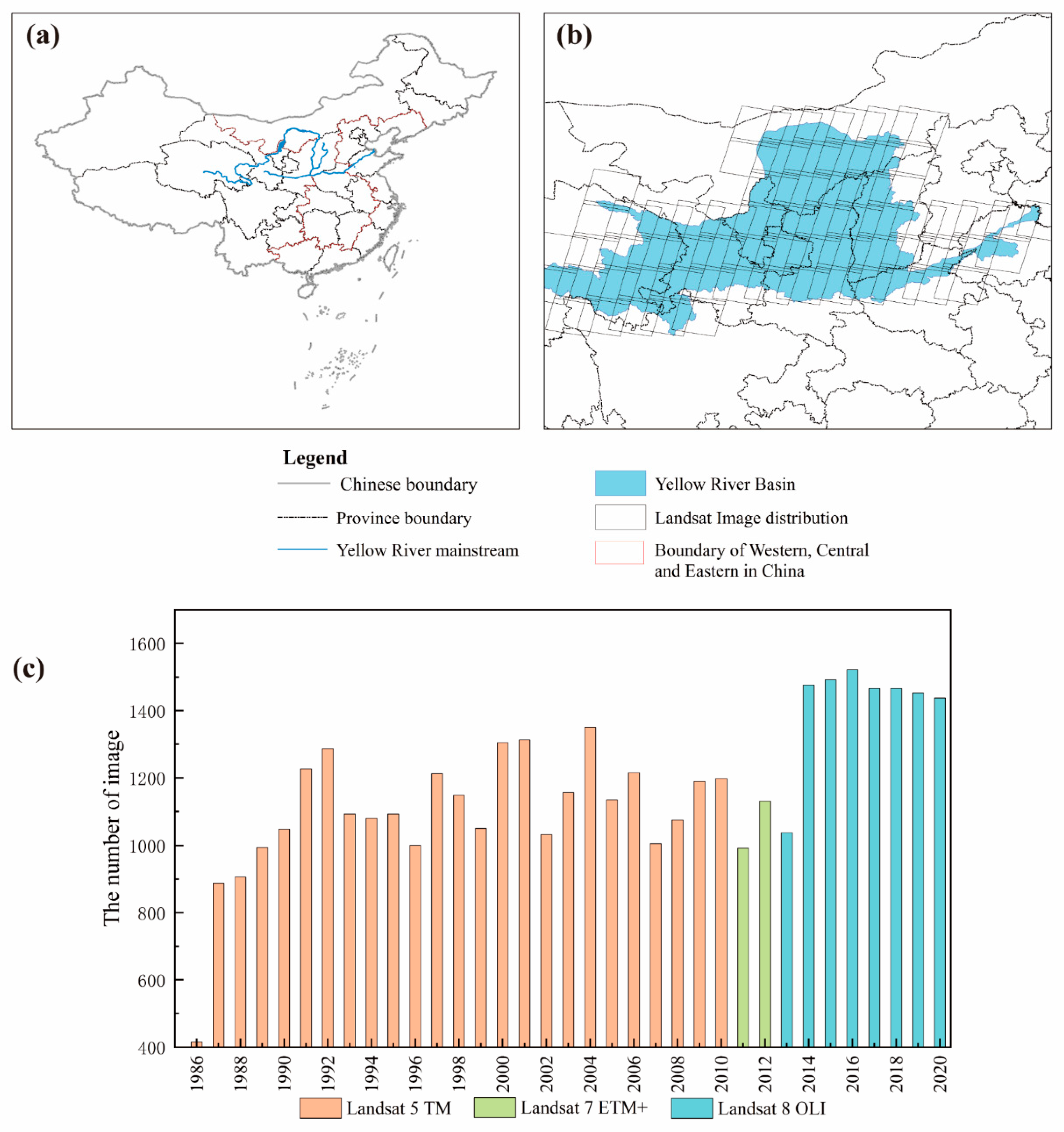
2.1. Study Area

Yellow River, the second longest river in China, flows from west to east through nine provinces and straddles four geomorphic units (Figure 1a). The river is about 5464 km long with a basin area of over 700,000 km² [43]. The Yellow River Basin is an important area of agricultural and economic development and is rich in mineral and water resources. In addition, the YRB has 12 important national ecological function areas. Hence, it has become a vital ecological security protection barrier and provides essential support for landscape construction. The Outline of the Yellow River Basin’s Ecological Protection and High-quality Development Plan pointed out that the greatest weakness in the ecology of the region was inadequate high-quality development and the main problem was ecological fragility [44]. The development of regions and provinces along the Yellow River is out of balance, and ecological conditions are poor with a fragmented environmental carrying capacity for natural resources. In view of the above information, it is appropriate to research urban and rural development in the YRB.

Since the YRB is an important economic belt in China, human activities therein possess the characteristics of high intensity, wide range, and long history. With the recent rapid economic development and the acceleration of urbanization in the region, the proportion of IS such as residential, transportation, and industrial land has rapidly increased. An urgent need exists to thoroughly understand the current situation and the process involved in IS expansion so that land planners and managers can master the changes in IS and develop the necessary analyses and research regarding the ecological effects of EIS.

Figure 1. Locations of: (a) the Yellow River Basin (YRB) within a map of the major administrative boundaries in China; (b) path/row of Landsat imagery used in the study area. (c) Distribution of the annual number of Landsat images used in the study.

Figure 1. Locations of: (a) the Yellow River Basin (YRB) within a map of the major administrative boundaries in China; (b) path/row of Landsat imagery used in the study area. (c) Distribution of the annual number of Landsat images used in the study.

Note: shapefiles of boundaries were downloaded from the National Catalogue Service for Geographic Information; the Landsat WRS 2 Descending Path Row Shapefile was downloaded from the United States Geological Survey.

2.2. Data

2.2.1. Landsat Data

We used Landsat data to create a binary classification of IS and non-IS areas and to establish the remote sensing-based ecological index (RSEI). Landsat data were provided by the United States Geological Survey (USGS) and the National Aeronautics and Space Administration (NASA). Different ranks of Landsat data were archived in the GEE platform by hierarchical structure naming: compared with Collection 1, Collection 2 adopts the latest data processing algorithms and methods; Level-2 is to add atmospheric correction steps based on Level-1 geometric correction and radiometric calibration; and the difference between Tier 1 and Tier 2 lies in whether orthorectification was used. In this paper, Landsat 5, 7, and 8 of “/C02/T1_L2” were selected for use.

2.2.2. NTL Data

The NOAA/VIIRS/DNB/MONTHLY_V1/VCMSLCFG in the GEE provides monthly composite data, which uses stray light correction procedures to expand data coverage [45]. The data include two bands: “avg_rad” and “cf_cvg”. The former is the monthly average day/night band (DNB) radiation value, and the latter is the total number of observations included in each pixel. In this paper, the average DNBs of 2020 in the GEE platform were used as a mask to mitigate uncertainties in classification.

2.2.3. Impervious Surfaces Products

In this paper, three IS products were used to validate the impervious surfaces maps of the Yellow River Basin (IS-YRB) from 1990, 1995, 2000, 2005, 2010, and 2015. Only independent IS products were considered. Additionally, the selected products should be obtained from different data processing methods than IS-YRB and have high accuracy. Upon comprehensive consideration, the following products were selected.

GAIA was obtained by Gong et al. [2], and the data were based on 583 global geographic grids (including 155 arid regions), which were divided into 3.5° × 3.5° units (source: http://data.ess.tsinghua.edu.cn/gaia.html (accessed on 15 March 2021)). To effectively reduce the misclassification of bare land and IS in arid regions, arid and non-arid regions were identified using respective binary classification methods.

The Normalized Urban Areas Composite Index (NUACI) algorithm was proposed by Liu et al. [22]. The NUACI was established through the combination of NTL, Normalized Difference Water Index (NDWI), NDVI, Normalized Difference Built-up Index (NDBI), and partition threshold segmentation to obtain urban data (source: http://www.geosimulation.cn/GlobalUrbanLand.html (accessed on 1 January 2021)). Here, we refer to the global-urban-data-based NUACI algorithm using the term NUACI.

The Global Annual Urban Dynamics (GAUD) was a derivative dataset from NUACI, and it was also provided by Liu et al. [46]. It was produced by incorporating four global IS products to map data for 1985 and 2015. The NUACI algorithm and temporal segmentation approach were then developed for mapping annual urban dynamics (source: https://doi.org/10.6084/m9.figshare.11513178.v1 (accessed on 15 March 2021).

2.2.4. Other Auxiliary Data

We collected urban boundary data for 1990 and 2018 from the Global Urban Boundary (GUB) database (source: http://data.ess.tsinghua.edu.cn/gub.html (accessed on 15 March 2021)). This dataset was obtained based on GAIA, which was developed by kernel density estimation along with cellular automata and morphology methods [47]. In addition to the abovementioned data, all boundary shapefiles were also required. Moreover, Sentinel-2 data for 2015 was downloaded from the GEE platform (provided by Scientific Hub, Copernicus) as a reference for comparison between data products.

2.3. Methodology

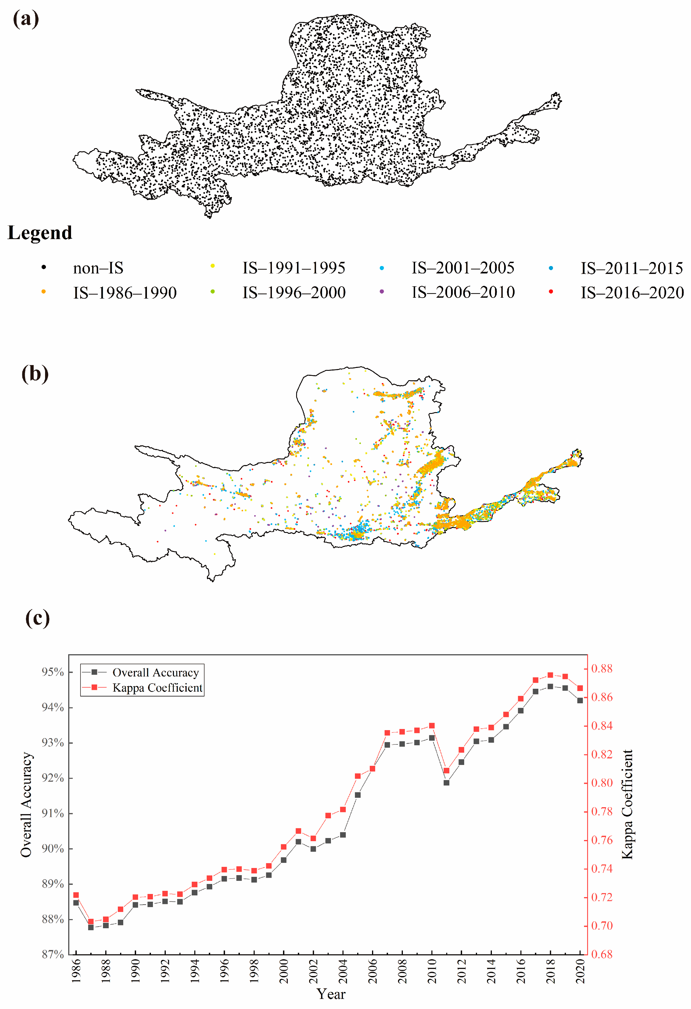
2.3.1. Binary Classification

(1) Preprocessing

Preprocessing included imagery cloud removal, data composition, and water masking. Before implementing imagery cloud removal, imagery should be selected with a boundary and date by the functions. In addition, a bitwise calculation was performed on quality assurance (QA) bands to filter out bad pixels and achieve the effect of removing clouds or cloud shadows. Annual median composite imagery was then obtained. Finally, a water mask layer was accomplished based on Equations (1) to (4) [48]:

$$\left(MNDWI>NDVI or MNDWI>EVI\right) and (EVI<0.1)$$

(1)

where $MNDWI$, $NDVI,$ and $EVI$ were calculated according to:

$$MNDWI=\left(Green-SWIR\right)/\left(Green+SWIR\right)$$

(2)

$$NDVI=\left(NIR-Red\right)/\left(NIR+Red\right)$$

(3)

$$EVI=\left(2.5\ast \left(\left(NIR-Red\right)/\left(NIR+6\ast Red-7.5\ast Blue+1\right)\right)\right)$$

(4)

where $Green$, $SWIR$, $NIR$, $Red$, $Blue$ indicate green, shortwave infrared, near-infrared, red, and blue surface reflectance, respectively.

(2) Feature selection

Spectral bands and spectral indices were chosen to constitute the feature set. Spectral bands covered all bands of multispectral imagery, while MNDWI (Modified NDWI), NDVI, and NDBI were designated as spectral indices. Reference Equations (2), (3), and (5) were used for the calculation of MNDWI, NDVI, and NDBI, respectively. It was difficult to separate IS from bare land by spectral information alone, but texture features provided the possibility of doing this [49,50]. Here, the Gray Level Co-occurrence Matrix was called in the GEE by function.

$$NDBI=\left(SWIR-NIR\right)/\left(SWIR+NIR\right)$$

(5)

(3) Sampling

According to the research objectives, the ground objects were divided into IS and non-IS (vegetation, bare land, water, wetland, etc.). The sample sets were selected by combining NTL imagery, Landsat imagery, and historical Google Earth imagery. Taking regional differences and phase changes into consideration, samples should obey the principle of widely representing ground objects. Hence, sample selection was carried out in the west, center, and east of the YRB individually at an interval of five years (1986, 1991, 1996, 2001, 2006, 2011, and 2016). Sample sets included points and polygons and can be seen in

Table 1. Numbers and types of samples.

		Points	Polygons	Total
Samples of pervious surface		7500	1000	8500
Samples of impervious surface	1986–2000	1350	150	1500
	2001–2005	1350	350	1700
	2006–2010	1350	550	1900
	2011–2020	1350	750	2100

.

(4) Classification

The Random Forests approach was proposed by Breiman [51,52]. The principle of RF is to construct a decision tree by selecting features after repeated random sampling with replacement. Multiple decision trees are repeatedly generated to form a random forest, and optimal classification results are generated by equal voting for input variable X. The number of decision trees and the number of feature variables are two important parameters of RF, and proper parameter setting ensures high-efficiency classification and avoids over-fitting. The RF algorithm is encapsulated in the GEE, and the command can be directly invoked. Here, the number of decision trees was determined through experiments, the number of characteristic variables was set as the square root of the input variables, and the remaining parameters were kept at default values.

(5) Postprocessing

After the above steps, initial image classification is obtained. To give the dataset high spatiotemporal consistency, the Temporal Consistency Check (TCC) was adopted. According to Dr. Li, TCC consists of two steps: temporal filtering and logical reasoning [53]. The basis of temporal filtering is that the IS and non-IS do not appear alternately in the three adjacent years; the logical reasoning is required in situations where a continuous IS for a period of time and a continuous non-IS for a period of time appear in an alternating pattern. The process of TCC is based on the following referenced literature [25,53,54].

2.3.2. Accuracy Assessment

Validation samples used to calculate quantitative metrics are usually used to analyze the accuracy of results, which can be referred to as “pixel-based”. Overall accuracy (OA) and kappa coefficient were selected for assessing the mapping results of impervious surfaces in the Yellow River Basin. The validation dataset had 214,000 points, including 4600 non-IS points and 2400 IS points (updated every five years) (Figure 2a,b). Evaluating the consistency and fit between the IS-YRB and existing products is also a method for assessing accuracy [20], which can be referred to as “fraction-based”. Specifically, all images were resampled to a resolution of 0.05° × 0.05°, and regional statistics were then performed to obtain the fraction of IS areas. The root mean square error (RMSE) and coefficient of determination (R²) were taken as judgment indicators to map scatterplots of the linear regression between different products.

2.3.3. Spatiotemporal Dynamics

The IS areas of the YRB, the west, center, and east of the YRB, and the provincial capitals were calculated annually from 1986 to 2020, and the impervious surfaces coverage rate within each research unit was also calculated. Compared with the binary imagery, the fraction density map can better show the degree of aggregation of IS pixels. Intentionally, the imagery was aggregated to 1 km × 1 km, and the fraction density maps of IS were then drawn by percentage. Next, the results were graded according to [0, 0.5], [0.5, 0.6], [0.6, 0.7], [0.7, 0.8], [0.8, 0.9] and [0.9, 1]. The variation trend of the fraction density maps was expressed by a least-squares regression slope, and the significance was tested by p-value.

In addition, the following two indices were selected to analyze the EIS in different research units during the research periods: expansion speed (ES) and expansion intensity (EI). These were calculated as follows:

$$\mathrm{ES}=\frac{S_{end}-S_{start}}{D}$$

(6)

$$\mathrm{EI}=\left[{\left(\frac{S_{end}}{S_{start}}\right)}^{\frac{1}{D}}-1\right]\ast 100\%$$

(7)

where $S_{start}$ and $S_{end}$ are the initial and final areas of IS, respectively, and $D$ is the time interval.

2.3.4. Construct RSEI

The RSEI index was calculated in this section based on Landsat. The main processing method involved normalizing the four variables (NDVI, wetness (WET), land surface temperature (LST), and Normalized Difference Built-up and Soil Index (NDBSI)). Next, compressed feature information was obtained through principal component analysis (PCA). Finally, the first principal component (PC1) was used to create the RSEI because it can efficiently integrate information of each indicator and can explain it reasonably. To demonstrate the environmental quality of the YRB, RSEIs for 1986, 1990, 2000, 2010, and 2020 were established following the steps mentioned in references [35,55]. Importantly, the following data processing details need to be emphasized: (1) the growing season (May–October) was selected for acquiring the imagery, and the target year was averaged based on three years of data (one year before, during, and after the target year) to minimize the effects of any data gaps caused by the removal of clouds; (2) during the normalization process, the minimum and maximum values were set to the 1st and 99th quantiles of the index values arranged in ascending order [36].

2.3.5. IS and RSEI

In this study, the RSEI value reflects the state of the ecosystem of the region area. In order to compare the IS and RSEI, different stable areas were set. Briefly, we first defined the GUB-1990 as the core urban areas (the circle1), and the areas between the GUB-1990 and the GUB-2018 as the urban development zone or suburban areas (the circle2) [56]. We then generated additional circles with the buffer size with the GUB-2018 as the benchmark [7]. We selected 1 km as the buffer width due to the spatial resolution of data and referring to the existing literature [7,39]. Because areas in different cities intersect when there are more than eight additional circles, we only set ten circles. Using these circle boundaries, we compared the IS coverage rate and the mean RSEI value. In addition, we counted the proportional of the RSEI rating.

3. Results

3.1. Accuracy Assessment of the Classification Results

3.1.1. Based on Validation Samples

Figure 2c shows that the OA of IS-YRB was 87–95%, with a kappa coefficient of 0.70–0.88. Generally, the values of OA and kappa coefficients were simultaneously increased over time. The one exception was in 2011, when the accuracy was lower than certain previous years (although it was within the bounds of credibility). Because high-resolution imagery and other supplementary data of the early years are lacking, training samples in the early period (especially before 2000) were selected only based on Landsat imagery with a resolution of 30 m, which inevitably led to errors. The efficiency and accuracy of the Random Forest classifier were reduced by the deviation of training samples. The sudden decrease in 2011 was also closely related to the selection of training samples. Furthermore, another main reason for classification errors was the massive number of mixed pixels, which often appear in the areas with low IS coverage. Nonetheless, the average OA and kappa coefficient observed in this paper were 90.93% and 0.79, respectively, indicating that the IS-YRB has a high degree of reliability.

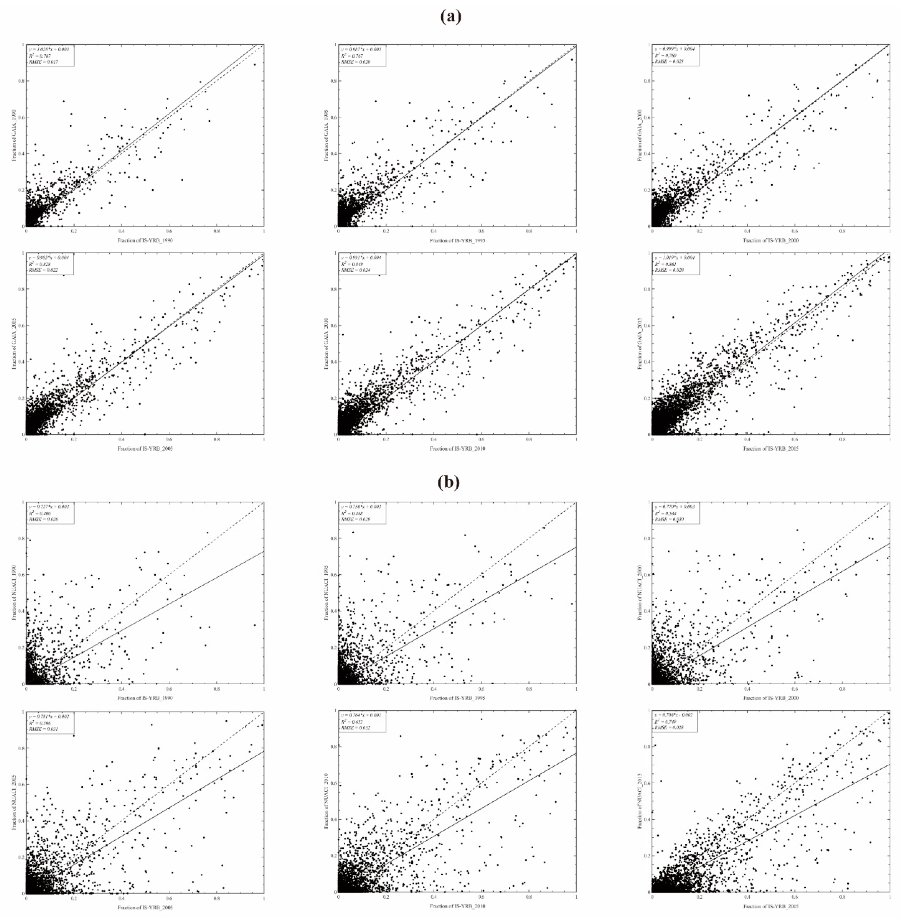
3.1.2. Based on Impervious Surfaces Products

To further quantitatively evaluate the accuracy of the extraction results, the spatial agreement between IS-YRB and GAIA/NUACI was demonstrated by scatterplots. Figure 3a illustrates that the data between IS-YRB and GAIA (R² > 0.76, RMSE < 0.3, and slope close to 1) were in excellent agreement. Similarly, Figure 3b indicates the correlation between IS-YRB and NUACI, where it was found that the R² was lower than 0.75 and the slope was only close to about 0.75, which represented a moderate correlation between the two (RMSE < 0.32).

Comparing the IS-YRB and GAIA scatterplot with the IS-YRB and NUACI scatterplot, the former had higher spatial consistency. Notably, the remarkable differences between the former were interpreted in the “low coverage” areas (approaching the origin of coordinates). This finding was attributed to two errors: the commission errors driven by the suboptimal threshold that leads to much bare or cultivated land being regarded as impervious pixels in GAIA [25] and the omission error driven by the classification error mentioned in Section 3.1.1. Meanwhile, this shows that the scatter points are chaotic and irregular on either side of the regression line in the IS-YRB and NUACI scatterplot. Nevertheless, the NUACI-2015 revealed a significant underestimation problem, so the scatter points are mostly plotted below the 1:1 line. Zhang et al. [20] and Sun et al. [57] demonstrated that NUACI failed to correctly identify IS for some small, fragmented villages and roads.

3.2. Analysis of Impervious Surfaces Dynamics

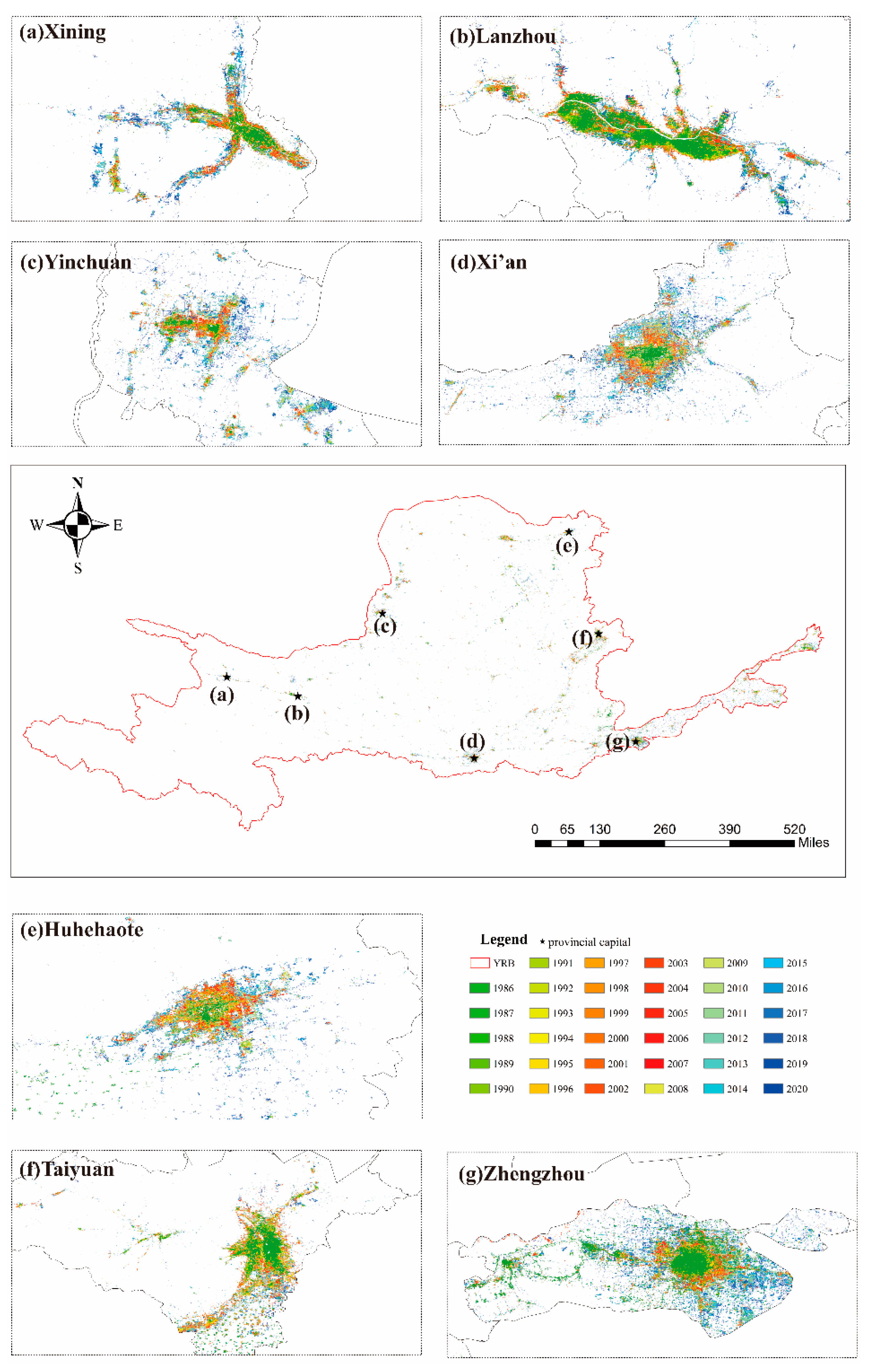
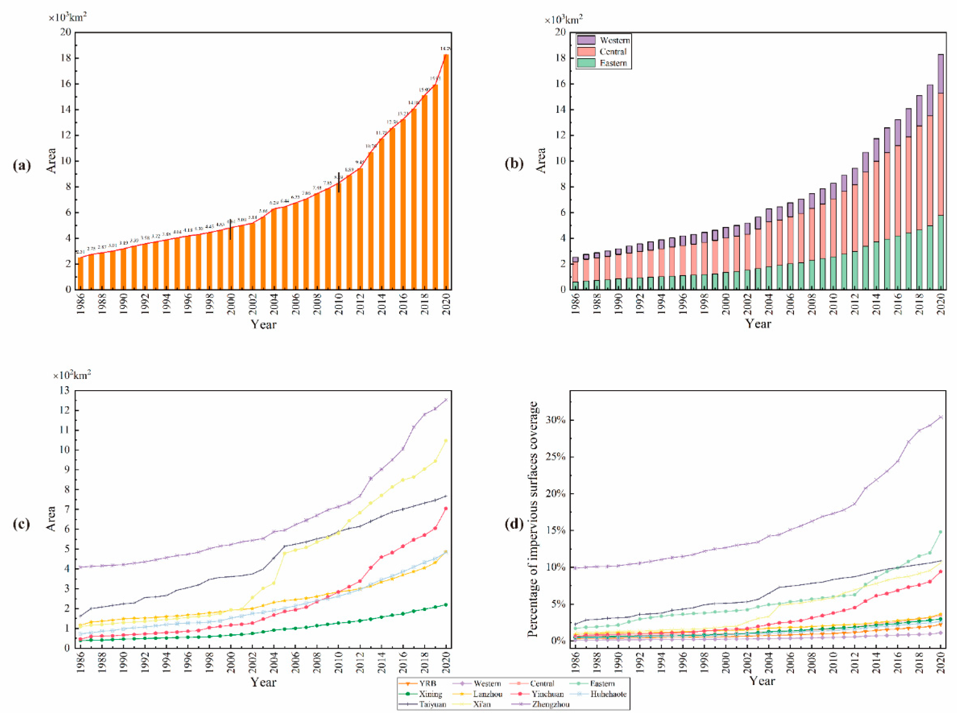
3.2.1. Annual Impervious Surfaces Dynamics

From the perspective of spatial distribution, the IS pixels that were added later over time mostly surrounded the original IS pixels (Figure 4). The IS areas of the entire YRB increased to 18,287.36 km² in 2020 compared to 2513.71 km² in 1986, increasing by about 463 km²/a. Further investigation of Figure 5a revealed the conclusion that IS areas grew slowly at a rate of 166 km²/a from 1986 to 2000, while the first rapid growth occurred between 2001 and 2010 at the rate of 365 km²/a. IS areas experienced another period of accelerated growth from 2011 to 2020, which the growth rate was 1044 km²/a. It is well known that there is a wide gap in the development of different parts of the YRB; therefore, the YRB was decollated into western, central, and eastern regions under the policy definition (Figure 1a). Moreover, annual changes in IS areas in provincial capitals were calculated and mapped in Figure 5c. The results suggest that Zhengzhou has always had the most IS areas, followed by Taiyuan or Xi’an. In the years between 2000 and 2005, the IS areas in Xi’an increased dramatically to rank second while the IS areas of other western cities such as Yinchuan and Xining increased steadily, which could reveal the promotion of growth of IS areas by the development of the western region in China starting from about the year 2000.

To better evaluate the relative status of IS coverage in different regions and provincial capitals, the ratios between the areas of IS and the research units can be found in Figure 5d. The results imply that the IS coverage rate in the central region was only slightly higher than in the YRB generally, although the provincial capitals had much higher percentages of IS than other areas. This provides strong evidence that the urban development of Shanxi and Henan was unbalanced. Interestingly, against the statistics, the IS areas in Yinchuan outstripped Lanzhou in 2010 (Figure 5c), and the IS coverage rate in Yinchuan overtook Lanzhou in 2000 (Figure 5d).

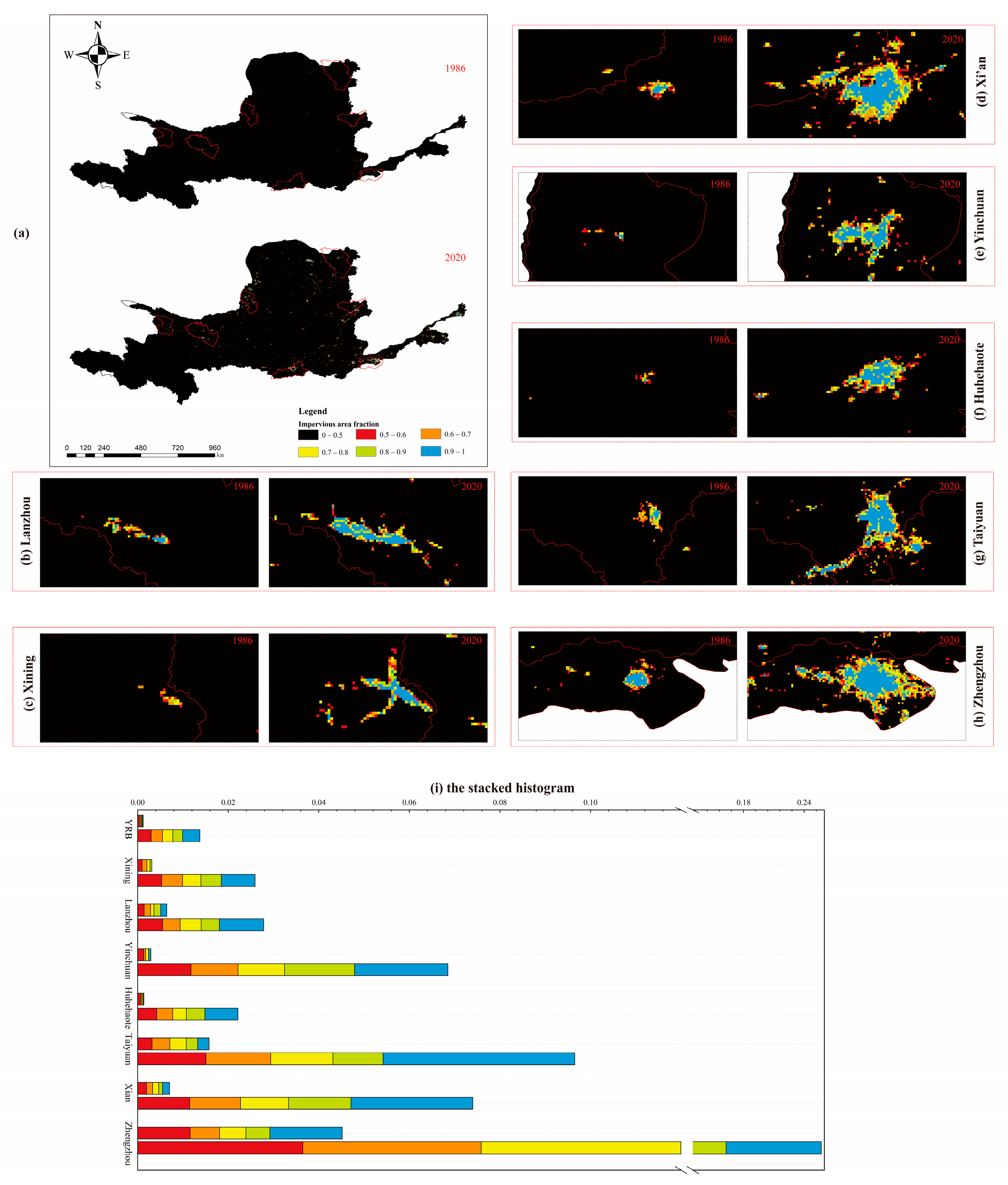
3.2.2. Comparison of Impervious Surfaces Fraction

Drawing references from previous theoretical frameworks for IS change detection [11,58], we reclassified the binary maps to 1 km × 1 km to calculate the impervious surfaces fraction (ISF) and then figured out the relational analysis between earlier time points and latest time points as intuitively as possible. The ISF for 1986 and 2020 are illustrated in Figure 6 by six degrees with a sequential color scheme. In either 1986 or 2020, the ISF showed a trend of decreasing from the urban core areas to the surrounding areas. By comparing across the maps, it was revealed that the ISF increased considerably from 1986 to 2020, which represents the expansion that could be distinctly perceived in the urban core areas. It is clear from the stacked histogram that the ISF at all degrees had improved to varying degrees, representing densification and expansion. Visual interpretation and frequency statistical analysis of the ISF provided some information related to the spatiotemporal variation in IS, but they failed to reveal the expansion and densification processes. The solution was to use least-squares regression.

Figure 7 shows the ISF of the interannual change trend by slope ([0, 0.01], [0.01, 0.02], [0.02, 0.03], [0.03, 0.04], and [0.04, 1], with p < 0.05). What stands out in the figure is that the significant trend of ISF can be summarized as increasing first and then decreasing from the center to surrounding areas for each prefectural city. According to this phenomenon, the areas can be divided from the prefectural center into the first, second, and third circles.

By combining Figure 6 and Figure 7, we described three circles as follows: (1) for the first circle—the core urban areas—the ISF in the initial was high, so the internal filling and development of space was limited, and the rate of change was small; (2) for the second circle—the suburban or rural areas—the ISF in the initial was low, but as the urban areas gradually expanded outward, the external extension space was large, and the rate of change was significant; (3) for the third circle—the exurb rural or depopulated areas—the ISF in the initial was nearly zero, the growth of IS originated from the original bare land or farmland, which was sometimes converted into a new town or the edge of a town, and the rate of change was obvious but not significant. Consequently, the ISF in 1986, the change from 1986 to 2020, and the ISF in 2020 among three circles can be described as “high coverage–low change–high coverage”, “low coverage–high change–high coverage” and “low coverage–medium change–low coverage”, respectively.

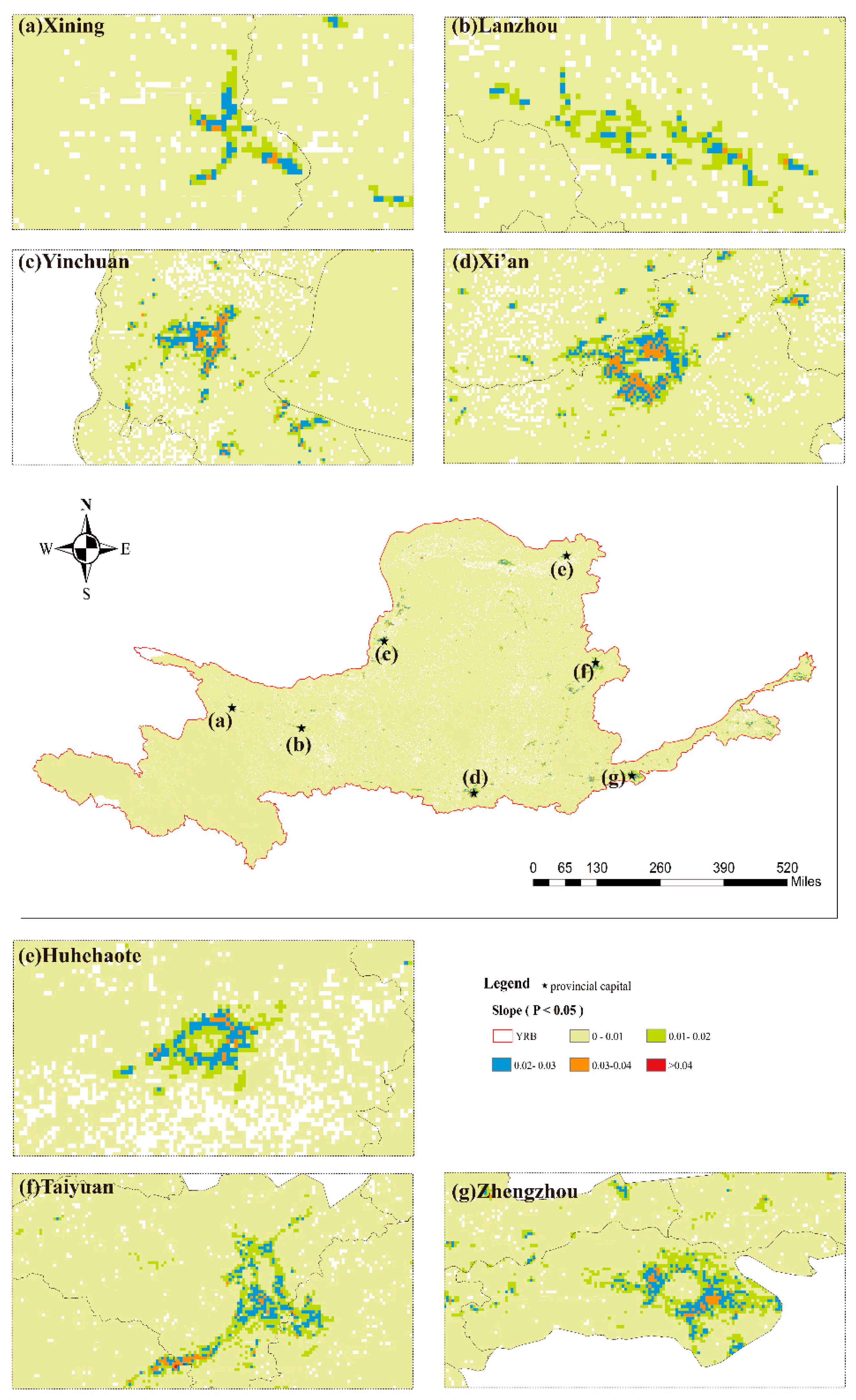
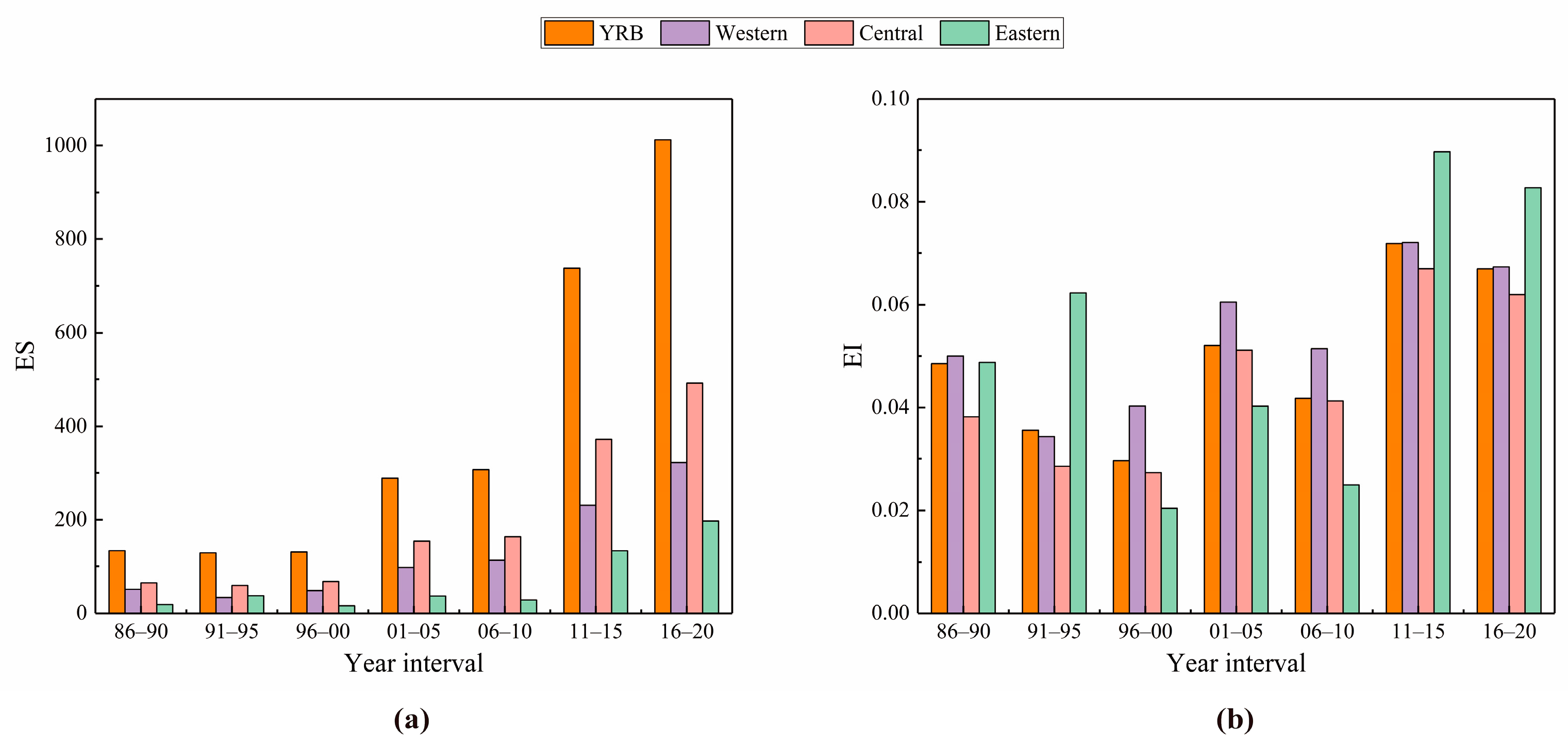
3.2.3. Evaluation of Impervious Surfaces Expansion from 1986 to 2020

We analyzed the EIS at intervals of five years; the results are shown in Figure 8 and Tables S1 and S2. In Figure 8a, the values of ES in the YRB have obvious time differences, with step-like increases at the transformed points of 2000 and 2010. The results strongly confirm the description of the three growth stages described above in Section 3.2.1. The values of ES in the western and central parts of the YRB were basically in line with the stepped increasing trend, except in the Ordos (Table S1). However, the values of ES in the eastern areas increased suddenly after 2010, so this region doesn’t have the characteristic of having three distinct periods. Table S1 indicates that the values of ES in capital cities were usually higher than those in non-capital cities, reflecting the regional imbalance of urban development.

In the same way, the values of EI are shown in Figure 8b and Table S2. Overall, the values of EI fell between 0.02 and 0.09, showing an increase with irregular oblique fluctuations and the peak occurring in 2011–2015. It was also found that the value of EI in 2001–2005 was greater than in 1996–2000 or 2006–2010. Moreover, the value of EI in eastern areas initially and sensitively peaked in 1991–1995 due to the comprehensive development of the Yellow River Delta beginning in this period. In general, statistics from the values of EI showed three phases, which corresponded to the description in Section 3.1.1, with a downward trend in each period and an upward trend between periods.

These results indicated that the EIS could be analyzed for three periods to better understand the EIS: slow growth from 1986 to 2000, rapid growth from 2001 to 2010, accelerated growth from 2011 to 2020, and a downward trend in each period. In addition, the results demonstrated that the expansion trends of IS in the western and central areas were synchronized with that of the entire YRB.

3.3. Analysis of the Effects of Impervious Surfaces Expansion by RSEI

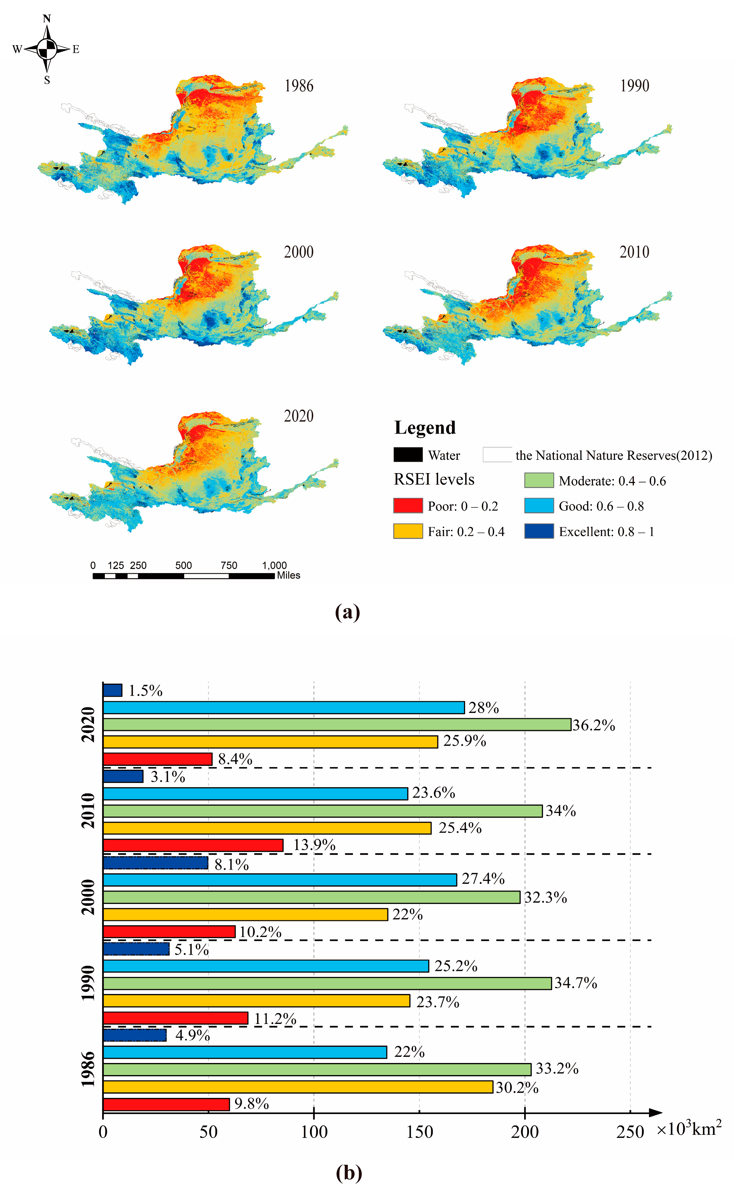
3.3.1. Ecological Status in the YRB

A principal component analysis showed the loads of four indices and the weight of their influence on the environment. The loads of four indices in PC1 are presented in

Table 2. Loads and contributions of indices to PC1.

Year	PC1				Contribution
	NDVI	WET	LST	NDBSI
1986	0.33280	0.69872	−0.60621	−0.18315	65.2721
1990	0.31870	0.72534	−0.57887	−0.19293	73.4465
2000	0.42276	0.58320	−0.65819	−0.21894	73.2763
2010	0.40444	0.71649	−0.51518	−0.24013	76.8011
2020	0.47879	0.67823	−0.48274	−0.27880	73.0507

Note: PC1, Principal Component 1; NDVI, Normalized Difference Vegetation Index; WET, Wetness Index; LST, Land Surface Temperature Index); NDBSI, Normalized Difference Built-up and Soil Index.

; there were distinct positive and negative differences. The loads of NDVI and WET were positive, denoting that the two indices contributed to an improvement of the ecological environment. The negative loads of LST and NDBSI indicated that the two indices had inhibitory effects on ecological improvement. In addition, PC1 contained most of the characteristic information of the four indices (Table 2), which means that it could be used to construct the RSEI.

Figure 9a displays the spatial distribution of the RSEI (poor: 0 < RSEI < 0.2; fair: 0.2 ≤ RSEI <0.4; moderate: 0.4 ≤ RSEI < 0.6; good: 0.6 ≤ RSEI < 0.8; excellent: 0.8 ≤ RSEI ≤ 1). Areas with a poor environment commonly occurred near or in the Ordos Plateau and Tengger Desert. The fair areas were next to the poor areas and occupied the north or west of Yulin, Qingyang, and Guyuan as well as the southeast of Dingxi and Lanzhou. The areas with moderate and good environmental conditions were distributed in the source region of the yellow river, Ningxia Plain, and Hetao Plain as well as in the downstream region. The areas with excellent conditions were largely concentrated in and around the National Nature Reserves (Figure 9a).

The average RSEI values were 0.465 (1986), 0.478 (1990), 0.502 (2000, the maximum RSEI), 0.454 (2010, the minimum RSEI) and 0.477 (2020). The average RSEI of the YRB increased from 1986 to 2000 and initially decreased and then increased from 2000 to 2020. To determine the overall changes in the average RSEI from 1986 to 2020, the spatial area of each level could be determined using Figure 9b. The areas with poor and fair conditions accounted 40%, 34.9%, 32.2%, 39.3%, and 34.2% during the respective time intervals from 1986 to 2020, which indicates a decreasing trend with an abrupt rise in 2010. The areas with moderate and good environmental conditions accounting for over half of the entire region fluctuated during 1986–2020 and reached its lowest proportion in 2010 (57.6%) and its highest proportion in 2020 (64.2%). The original proportion in 1986 was 55.2%. Theoretically, with the increase of the National Nature Reserves and the improvement of environmental protection and public awareness, the areas with excellent conditions should continue to increase. However, the change of excellent areas varied, with some previously excellent areas degenerating to good environmental conditions over time. Nonetheless, the excellent areas were really small. Consequently, it can be concluded that the environmental quality of the YRB has shown a trend of improvement from 1986 to 2020.

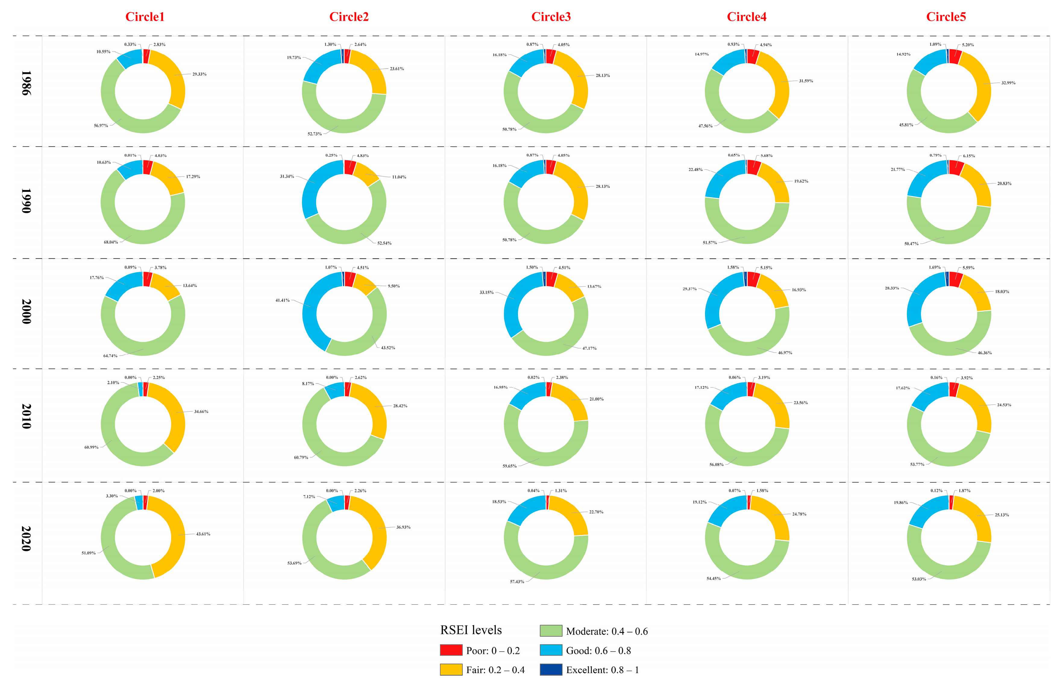
3.3.2. The Effects of IS change on RSEI

It is apparent that the IS coverage rate (ISCR) in each circle increased over time and decreased progressively in each time node over the circle (

Table 3. ISCR and RSEI_mean of different circles in 1986, 1990, 2000, 2010, and 2020.

Circle	1986		1990		2000		2010		2020
	ISCR	RSEImean	ISCR	RSEImean	ISCR	RSEImean	ISCR	RSEImean	ISCR	RSEImean
1	2.2281	0.4516	2.8231	0.4725	4.2871	0.4958	7.3249	0.4207	16.0866	0.4119
2	2.0486	0.4782 *	2.5960	0.5111 *	3.9433	0.5363 *	6.7495	0.4404	14.8637	0.4269
3	2.0428	0.4706	2.5884	0.5063	3.9317	0.5313	6.7297	0.4619	14.8246	0.4571
4	2.0369	0.4647	2.5810	0.5003	3.9208	0.5250	6.7107	0.4655	14.7866	0.4645
5	2.0312	0.4606	2.5736	0.4957	3.9095	0.5202	6.6915	0.4667	14.7487	0.4685
6	2.0254	0.4579	2.5663	0.4924	3.8988	0.5167	6.6731	0.4673 *	14.7137	0.4712
7	2.0195	0.4556	2.5589	0.4895	3.8876	0.5137	6.6538	0.4672	14.6750	0.4729
8	2.0140	0.4538	2.5520	0.4871	3.8769	0.5112	6.6352	0.4667	14.6350	0.4742
9	2.0083	0.4527	2.5447	0.4853	3.8659	0.5092	6.6164	0.4664	14.5949	0.4754
10	2.0026	0.4517	2.5374	0.4836	3.8547	0.5075	6.5972	0.4659	14.5531	0.4763 *

Note: ISCR, impervious surface coverage rate; RSEI_mean, mean of RSEI; “*”repesents the maximum value for the corresponding year of the RSEI_mean.

). In contrast to the regular ISCR changes, the mean RSEI value (RSEI_mean) peaked in different circles (circle2 of 1986, 1990, and 2000; circle6 of 2010; and circle10 of 2020) over time but peaked in same time node over the circle (2000). Comparisons were made between every two adjacent years. Although there was a slight rising number of ISCR between 1986 and 1990 and between 1990 and 2000, the RSEI_mean values in 1990 or 2000 were still larger than that in 1986 or 1990, respectively. The difference in the RSEI_mean between 2000 and 2010 was the most salient, with a nearly 1.7 times difference in the ISCR. Compared with other adjacent years, the disparity in the ISCR exceeded two times between 2010 and 2020, but it accompanied minimal gaps in RSEI_mean values, whose changes were diverse.

Combined with the distribution characteristics of the ISCR and RSEI_mean in Table 3, the proportion of the corresponding RSEI levels at time nodes of various circles were calculated (Figure 10). From the perspective of the time scale, the proportion of poor RSEI levels showed a trend of undulating decrease, especially in circle5 (5.2% in 1986, 6.15% in 1990, 5.59% in 2000, 3.92% in 2010, and 1.87% in 2020), while the other levels showed disparateness. The proportion of good and excellent RSEI levels form 1986 to 2020 observably decreased in circle1 and circle2 (10.88% to 3.3%, and 21.03% to 7.12%, respectively), and volatility increased beyond circle3 (17.05% to 18.57%, 15.9% to 19.19%, and 16.01% to 19.98%).

The change of RSEI values of different ISCRs implied that the increase of impervious land had certain effects on the ecological environment. In reality, the densification and increase of IS caused damage to grassland and cropland. Additionally, in the process of replacing barren land with IS, the surrounding environment was artificially improved to ensure the livability of the region [56], and some newly built IS locations have become more and more “green” [59]. In summary, the sharp increase in ISCR usually exerts an adverse effect in RSEI, but this is not always the case. Furthermore, an undeniable positive effect occurred far from urban core areas.

4. Discussion

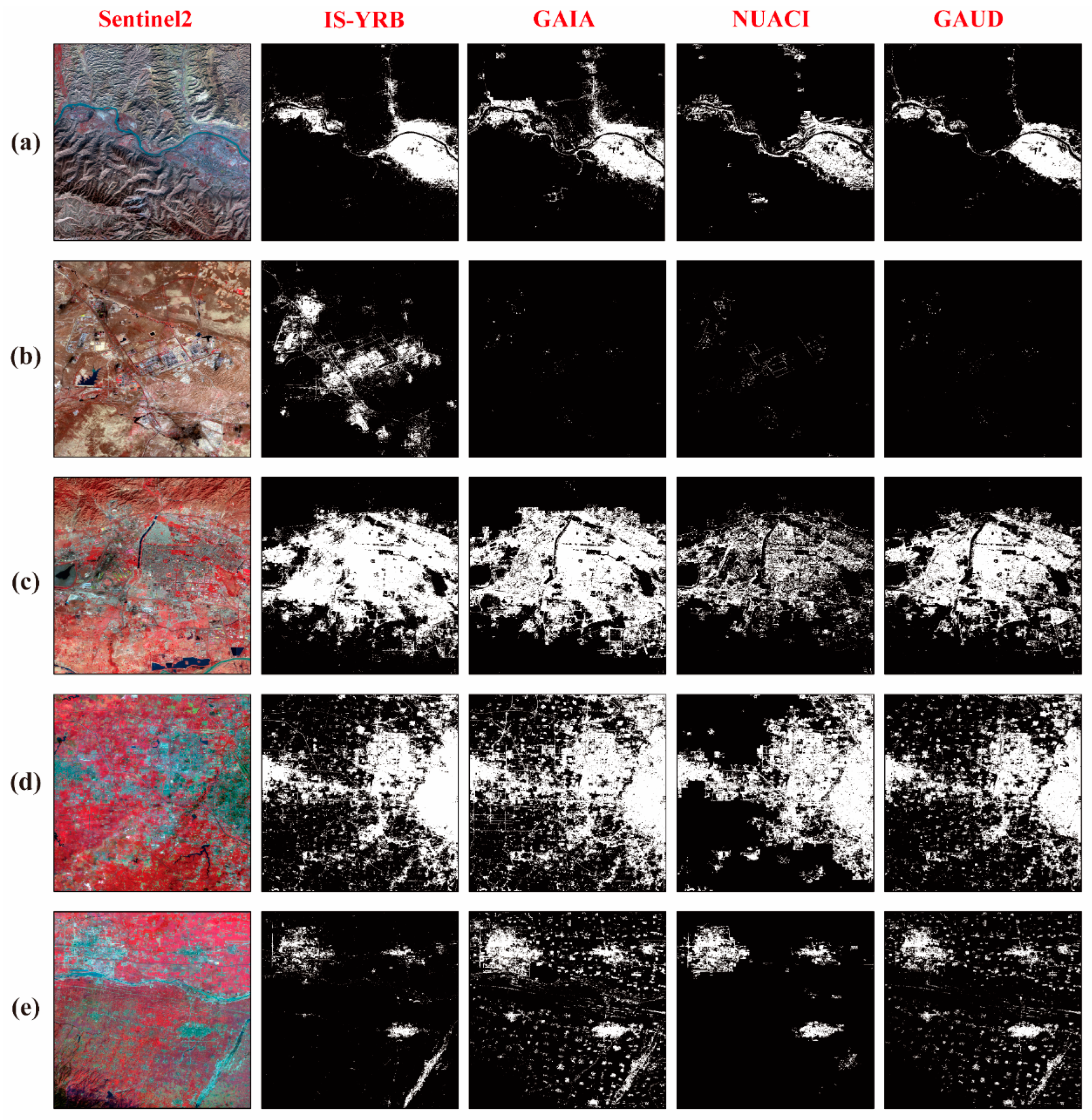
4.1. Comparison of the Results between IS-YRB with GAIA and NUACI/GAUD

As mentioned by Gong et al. [2], the thresholds of GAIA were based on 3.5° × 3.5° grids. It is possible, therefore, that a suboptimal threshold in local areas was applied and the details may have been blurred (Figure 11a,b). Li et al. [25] showed that a considerable amount of cultivated land was misclassified as IS in Guangzhou. In this study, we also found similar misclassified phenomena (bare land classified as IS) as seen in Figure 11a. Meanwhile, zooming in on the map of villages and towns disclosed significant differences between IS-YRB and GAIA (Figure 11d,e). Due to the limitation of the accuracy and the number of training samples collected in the YRB in rural areas, many IS pixels were missed. For further verification, we tried to fit the scattered points in IS-YRB and GAIA after stripping the village and town agglomeration areas (Figure S1a). Figure S1a shows that the R² of the fitting line between IS-YRB and GAIA increased significantly compared with that before villages and towns were excluded. The RMSE decreased in 2005, 2010, and 2015, but it increased in 1990, 1995, and 2000. The fluctuating change in RMSE did not mean a large discrepancy was observed between data products. It was interpreted as the value of RMSE being dominated by the difference between high-density points when low-density points completely prevail [60,61]. This comparative result, while preliminary, suggests that the agreement of IS-YRB and GAIA was improved after stripping the agglomeration areas of villages and towns. Thus, the main reason for the difference between IS-YRB and GAIA was the distant recognition ability in areas with low density and small coverage.

Combined with the previous introduction, IS-YRB was the supervised classification with post-classification processing, and NUACI was the threshold segmentation method based on a new index, while GAUD employed high precision auxiliary data incorporated with the NUACI algorithm and time-series segmentation. Although the NUACI algorithm took account of the differences in threshold values adopted in different areas, it was fragile in the face of the heterogeneity, which may be present within a few meters because of the complexity of the IS aggregation areas. The benchmark data in GAUD provide the guarantee of improved classification results; furthermore, change detection effectively solves the problems with the NUACI algorithm in heterogeneous regions. The scatter diagram in Figure S2 shows differences between the extraction results of NUACI and GAUD, and some points are even close to the X or Y axis. Likewise, contrastive diagrams of fitting lines between data before and after excluding villages and towns were drawn in Figure S1b. Figure S1b suggests that R² and RMSE of the fitting lines between IS-YRB and NUACI both increased. Regarding the distribution in the scatterplots, many scattered points are far away from the fitting lines, even when the density of the impervious surfaces was greater than 0.5. Consequently, we can infer that NUACI not only missed small villages and roads but also had a large amount of error associated with urban areas having a high density of impervious surface pixels. The improved method—GAUD—had a good consistency with IS-YRB (Figure S1b), which means that the NUACI algorithm needs to be combined with some assistant methods to optimize the rough classification results (Figure 11c,d,e). In conclusion, the main reason for the difference between IS-YRB and NUACI was the classification error caused by the immature extraction process of the latter, while the good fitting between IS-YRB and GAUD proved that different time series data extraction methods were both reliable (the former is an annual classification plus post-classification processing method, while the latter was a base year interpretation plus change detection method).

Through visual comparisons between the above data products, it was believed that IS-YRB is especially detailed in the high accumulation areas of IS, but the recognition effect in part of the rural areas such as small patches needs to be improved. Overall, the impervious surfaces dataset obtained by the RF and TCC is reliable.

4.2. Interpretation of the Variation of IS-YRB

The natural environment and human society both affect the variation in IS. These two completely different factors are not isolated but interact with each other and ultimately manifest themselves as the EIS.

Impervious surface areas are attached to the ground so that they are affected by terrain, habitat, resources, and other natural conditions. Although humans can transform the geographical environment (like Yan’an), variations in IS are still restricted by topography. For example, the terrain of Xining city is surrounded by mountains and lies at the intersection of three rivers; these landforms establish the city’s IS spatial pattern in the shape of an “X” (Figure 4a). However, the natural landform of Zhengzhou city located on a plain provides little restriction on the form of this urban area. Additionally, environmental carrying capacity is the paramount reason for urban development, which gave rise to a regional imbalance in the YRB during the entire study period. The “Ghost city”—Ordos—is a quintessential city that can be used to emphasize the impact of local resources on EIS. The Ordos is famous for its abundant coal and natural gas, which transformed it from a relatively underdeveloped, under-urbanized inland region to a high-profile, wealthy city [62]. After capital accumulation, the Kangbashi District of Ordos was designed as a new city that could accommodate a population of 1 million, although the population is currently only 150,000. Statistics show that 47 major construction projects were completed in Kangbashi between 2006 and 2009 alone, which explains the abnormal values of Ordos in Tables S1 and S2. This case also reveals the interaction of natural and human factors with the EIS.

Li et al. reported that the effects of natural factors on IS gradually weakened and determinants of urban expansion inclined to be more diverse over time [63]. Genuinely, the effects of human activities on EIS are complex and include transportation accessibility, service facility construction, and some major governmental policies. In each period, all human actions would have an effect, but something earthshaking would induce phase characteristics. The present study proposed and analyzed these possible major driving events.

From 1986 to 2000, the spatial extent of IS grew more slowly than in any other period from the results in Section 3.2. During this period, the government instituted family planning to limit population growth, and this began to produce results [64]. Undoubtedly, the population continued to expand rapidly. More residential areas and associated infrastructures were constructed on the unutilized land to provide essential living resources for residents. At the same time, economic system reform had relatively alleviated food and clothing problems. Since then, people tended to invest in their living conditions, giving rise to surface hardening. Therefore, we speculate that population expansion might be the major driving factor, and the underdeveloped economy might be the major restrained factor.

From 2000 to 2010, the IS continued to sprawl across the YRB; the growth of the spatial extent of IS areas accelerated more than it did between 1986 and 2000 no matter which research unit is considered in this paper. China’s economic system reform must still bring benefits to the expansion of IS, but it must do so without creating barriers because sufficient financial resources could be regulated and allocated by the government. The Western Development Strategy began in 2000, and the Rise of Central China was deployed in 2004. Under the guidance of development plans, industrial plants and transportation facilities were designed, and a considerable area of cultivated and bare land was converted to IS. Meanwhile, significant reform occurred in the regional housing policy. As a result, the ownership of houses became an opportunity for investment, and the real estate industry began to surge. With the demand from homebuyers, the core of urban and even suburban areas was rapidly occupied by the IS of commercial properties. Therefore, policy support and estate fever were reasonable and important factors contributing to the EIS between 2000 to 2010.

Starting from 2010 and again in 2020, the IS also expanded more rapidly. The effect of implementing the development of the western region in China and the rise of central China continued to contribute to the expansion of IS. Additionally, the industrial transfer policy accelerated the process of new-type industrialization and urbanization in the central and western regions of China. As shown in the urban system planning in the Yellow River Delta (2010–2020), structuring an urban system emphasized sound service facilities and urban–rural integration. In this period, efforts to eradicate poverty in the YRB achieved fruitful work. With the support of several national strategies and economic expansion, the spatial extent of IS in the YRB has increased to a new high (Figure 8). Therefore, we believe that government policy and economic conditions could be regarded as pivotal factors resulting in the changes in EIS between 2010 to 2020.

4.3. The Effect of EIS on Ecological Conditions in the YRB

In this study, spatial heterogeneity of ecological status in different geographical units of the YRB was identified. The results led to a similar conclusion, where the trend was positive for the regional environment [65]. During the expansion, the relationship among economic, social, and ecological variables was particularly complex [66]. The EIS is definitely regarded as one of the reasons for the degradation of habitat quality, and the impact of EIS extends beyond the physical boundaries of cities [7,67]. The phenomenon was shown in the period of dramatic expansion and in urban or suburban areas (Table 3 and Figure 8). Related studies also pointed out that EIS or urbanization brought pressure to the local environment [9,68,69]. It has also been observed that old urban areas generally showed improved environmental quality [56], and it is true that in order to meet the leisure and living environment needs of people, many ecological parks and health-care grasslands were developed after the urban IS density reached a certain level. Nevertheless, the coordinated development of urbanization and the ecological environment has hardly been achieved in many regions such as Heshuo County [69] and the YRB [41,42]. The negative influence of EIS on RSEI outside the urban periphery diminished in this study. This is consistent with the results of previous studies that showed that the implementation of strict protection and management in impervious construction can maintain and even improve the ecological quality of the region [56,59]. This can be interpreted as indicating the effectiveness of green development under efforts to create an ecologically sustainable civilization and the awareness of rational and long-term planning. This provides a reference for urban and rural planning; there is no need to emphasize blind “slimming”, but more attention should be paid to integrated design considering the reasonable proportion between the IS coverage rate and the need for ecological land. The suggestion is to shift from a growth model of urban expansion to one of internal optimization [56].

The complexity of ecosystems requres multiple indicators for the evaluation of ecological environment quality. However, the RSEI used in the present study contained only four indicators, and these were not sufficient for a comprehensive assessment of biodiversity and ecosystem characteristics. Despite this, the preliminary findings of this paper provide a theoretical basis for regional ecological protection and high-quality development. Using circular comparisons to reflect the influence of EIS on ecological conditions might not be specific enough. In future research, therefore, many indices, such as the species diversity index and air pollution index, will need to be added to construct a new RSEI index for comprehensive evaluation. Additionally, other perspectives and methods need to be further explored to analyze the direct and indirect response of the RSEI to EIS.

5. Conclusions

In this study, the Random Forest algorithm and Temporal Consistency Check were employed to identify impervious surfaces; this proved to be an effective way to map impervious surfaces on a large regional scale. The accuracy assessment and data comparison showed that our results could accurately delineate the impervious surfaces in the Yellow River Basin from 1986 to 2020, but mapping methods for small areas of IS require improvement, particularly in the early period.

Visual maps and statistical data were employed to understand the dynamics and differences of the impervious surfaces. From 1986 to 2020, impervious surface areas of the basin experienced a 463 km²/a increase. While slow growth from 1986 to 2000 was mostly driven by population expansion and an underdeveloped economy, rapid growth from 2001 to 2010 was mostly driven by policy support and estate fever, and accelerated growth from 2011 to 2020 was mostly driven by government policy and economic conditions. Moreover, the initial state and process changes and the final state of impervious surfaces from 1986 to 2020 were found to follow three patterns for the three areas described studied. These patterns consisted of “high coverage–low change–high coverage”, “low coverage–high change–high coverage” and “low coverage–medium change–low coverage”, corresponding to the core urban areas, the suburban or rural areas, and the exurb rural or depopulated areas, respectively. In addition, the differences in the expansion of impervious surfaces were significant in both inter-regional and intra-provincial analyses, such as when the western region was compared with the other regions or when Zhengzhou was compared with other cities in Henan. These results could enrich our knowledge about the spatiotemporal dynamics of impervious surfaces over the past three decades and provide scientific data and a theoretical basis for study of urbanization development and imbalance in the Yellow River Basin. Through the analysis of the RSEI, it was observed that the environmental quality of the entire basin showed an improvement trend with fluctuations. In addition, the densification of impervious surfaces undoubtedly contributed to the degradation of the regional environment, but the effect differed in core urban areas versus regions outside of urban areas. Adverse effects were prominent in the core urban areas, while regions outside the urban areas gradually showed an improved effect. This indicates the validity of the RSEI for evaluating eco-environmental quality, and it provides effective information for regional planning and coordinated development in the Yellow River Basin.

References

1. Weng, Q.H. Remote sensing of impervious surfaces in the urban areas: Requirements, methods, and trends. Remote Sens. Environ. 2012, 117, 34–49. [Google Scholar] [CrossRef]
2. Gong, P.; Li, X.C.; Wang, J.; Bai, Y.; Chen, B.; Hu, T.Y.; Liu, X.P.; Xu, B.; Yang, J.; Zhang, W.; et al. Annual maps of global artificial impervious area (GAIA) between 1985 and 2018. Remote Sens. Environ. 2020, 236, 111510. [Google Scholar] [CrossRef]
3. Yang, Q.Q.; Huang, X.; Yang, J.; Liu, Y. The relationship between land surface temperature and artificial impervious surface fraction in 682 global cities: Spatiotemporal variations and drivers. Environ. Res. Lett. 2021, 16, 024032. [Google Scholar] [CrossRef]
4. Lu, L.; Peng, G. Urban and air pollution: A multi-city study of long-term effects of urban landscape patterns on air quality trends. Sci. Rep. 2020, 10, 18618. [Google Scholar] [CrossRef]
5. Zhou, D.C.; Zhao, S.Q.; Zhang, L.X.; Liu, S.G. Remotely sensed assessment of urbanization effects on vegetation phenology in China’s 32 major cities. Remote Sens. Environ. 2016, 176, 272–281. [Google Scholar] [CrossRef] [Green Version]
6. Zheng, Z.H.; Wu, Z.F.; Yang, Z.W.; Francesco, M. Analyzing the ecological enviroment and urbanization characteristics of the Yangtze River Delta Urban Agglomeration based on Google Earth Engine. Acta Ecol. Sin. 2021, 41, 717–729. [Google Scholar] [CrossRef]
7. Du, J.Q.; Fu, Q.; Fang, S.F.; Wu, J.H.; He, P.; Quan, Z.J. Effects of rapid urbanization on vegetation cover in the metropolises of China over the last four decades. Ecol. Indic. 2019, 107, 105458. [Google Scholar] [CrossRef]
8. Song, Y.S.; Li, F.; Wang, X.K.; Xu, C.Q.; Zhang, J.Y.; Liu, X.S.; Zhang, H.X. The effects of urban impervious surfaces on eco-physiological characteristics of Ginkgo biloba: A case study from Beijing, China. Urban For. Urban Green 2015, 14, 1102–1109. [Google Scholar] [CrossRef]
9. Strohbach, M.W.; Doring, A.O.; Mock, M.; Sedrez, M.; Mumm, O.; Schneider, A.K.; Webers, S.; Schroder, B. The “Hidden Urbanization”: Trends of Impervious Surface in Low-Density Housing Developments and Resulting Impacts on the Water Balance, Front. Environ. Sci. Eng. 2019, 7, 29. [Google Scholar] [CrossRef] [Green Version]
10. Zhang, L.; Weng, Q.H.; Shao, Z.F. An evaluation of monthly impervious surface dynamics by fusing Landsat and MODIS time series in the Pearl River Delta, China, from 2000 to 2015. Remote Sens. Environ. 2017, 201, 99–114. [Google Scholar] [CrossRef]
11. Shahtahmassebi, A.R.; Song, J.; Zhang, Q.; Blackburn, G.A.; Wang, K.; Huang, L.Y.; Pan, Y.; Moore, N.; Shahtahmassebi, G.; Haghighi, R.S.; et al. Remote sensing of impervious surface growth: A framework for quantifying urban expansion and re-densification mechanisms. Int. J. Appl. Earth Obs. Geoinf. 2016, 46, 94–112. [Google Scholar] [CrossRef] [Green Version]
12. Elvidge, C.D.; Tuttlle, B.T.; Sutton, P.C.; Baugh, K.E.; Howard, A.T.; Milesi, C.; Bhaduri, B.L.; Nemani, R. Global Distribution and Density of Constructed Impervious Surfaces. Sensors 2007, 7, 1962–1979. [Google Scholar] [CrossRef] [PubMed]
13. Huang, X.M.; Schneider, A.; Friedl, M.A. Mapping sub-pixel urban expansion in China using MODIS and DMSP/OLS nighttime light. Remote Sens. Environ. 2016, 175, 92–108. [Google Scholar] [CrossRef]
14. Guo, W.; Li, G.Y.; Ni, W.J.; Zhang, Y.H.; Lu, D.S. Exploring improvement of impervious surface estimation at national scale through integration of nighttime light and Proba-V data, GISci. Remote Sens. 2018, 55, 699–717. [Google Scholar] [CrossRef]
15. Ma, Q.; He, C.Y.; Wu, J.G.; Liu, Z.F.; Zhang, Q.F.; Sun, Z.X. Quantifying spatiotemporal patterns of urban impervious surfaces in China: An improved assessment using nighttime light data. Landsc. Urban Plan. 2014, 13, 36–49. [Google Scholar] [CrossRef]
16. Huang, X.; Yang, J.J.; Li, J.Y.; Wen, D.W. Urban functional zone mapping by integrating high spatial resolution nighttime light and daytime multi-view imagery. ISPRS J. Photogramm. 2021, 175, 403–415. [Google Scholar] [CrossRef]
17. Zhang, Q.L.; Seto, K.C. Mapping urbanization dynamics at regional and global scales using multi-temporal DMSP/OLS nighttime light data. Remote Sens. Environ. 2021, 115, 2320–2329. [Google Scholar] [CrossRef]
18. Zhao, M.; Zhou, Y.Y.; Li, X.; Cao, W.T.; He, C.Y.; Yu, B.L.; Li, X.; Elvidge, C.; Cheng, W.M.; Zhou, C.H. Applications of Satellite Remote Sensing of Nighttime Light Observations: Advances, Challenges, and Perspectives. Remote Sens. 2019, 11, 1971. [Google Scholar] [CrossRef] [Green Version]
19. Gao, F.; De Colstoun, E.B.; Ma, R.H.; Weng, Q.H.; Masek, J.G.; Chen, J.; Pan, Y.Z.; Song, C.H. Mapping impervious surface expansion using medium-resolution satellite image time series: A case study in the Yangtze River Delta, China. Int. J. Remote Sens. 2012, 33, 7609–7628. [Google Scholar] [CrossRef]
20. Zhang, X.; Liu, L.Y.; Wu, C.S.; Chen, X.D.; Gao, Y.; Xie, S.; Zhang, B. Development of a global 30m impervious surface map using multisource and multitemporal remote sensing datasets with the Google Earth Engine platform. Earth Syst. Sci. Data 2020, 12, 1625–1648. [Google Scholar] [CrossRef]
21. Cao, X.M.; Gao, X.H.; Shen, Z.Y.; Li, R.X. Expansion of Urban Impervious Surfaces in Xining City Based on GEE and Landsat Time Series Data. IEEE Access 2020, 8, 147097–147111. [Google Scholar] [CrossRef]
22. Liu, X.P.; Hu, G.H.; Chen, Y.M.; Li, X.; Xu, X.C.; Li, S.Y.; Pei, F.S.; Wang, S.J. High-resolution multi-temporal mapping of global urban land using Landsat images based on the Google Earth Engine Platform. Remote Sens. Environ. 2018, 209, 227–239. [Google Scholar] [CrossRef]
23. Xu, H.Z.Y.; Wei, Y.C.; Liu, C.; Li, X.; Fang, H. A Scheme for the Long-Term Monitoring of Impervious−Relevant Land Disturbances Using High Frequency Landsat Archives and the Google Earth Engine. Remote Sens. 2019, 11, 1891. [Google Scholar] [CrossRef] [Green Version]
24. Gong, P.; Li, X.C.; Zhang, W. 40-Year (1978–2017) human settlement changes in China reflected by impervious surfaces from satellite remote sensing. Sci. Bull. 2019, 64, 756–763. [Google Scholar] [CrossRef] [Green Version]
25. Li, P.L.; Liu, X.P.; Huang, Y.H.; Zhang, H.H. Mapping impervious surface dynamics of Guangzhou downtown based on Google Earth Engine. J. Geo-Inf. Sci. 2020, 22, 638–648. [Google Scholar] [CrossRef]
26. Song, X.P.; Sexton, J.O.; Huang, C.Q.; Channan, S.; Townshend, J.R. Characterizing the magnitude, timing and duration of urban growth from time series of Landsat-based estimates of impervious cover. Remote Sens. Environ. 2016, 175, 1–13. [Google Scholar] [CrossRef]
27. Huang, X.; Li, J.Y.; Yang, J.; Zhang, Z.; Li, D.R.; Liu, X.P. 30 m global impervious surface area dynamics and urban expansion pattern observed by Landsat satellites: From 1972 to 2019. Sci. China Earth Sci. 2021, 64, 1922–1933. [Google Scholar] [CrossRef]
28. Liu, C.; Zhang, Q.; Luo, H.; Qi, S.H.; Tao, S.Q.; Xu, H.Z.Y.; Yao, Y. An efficient approach to capture continuous impervious surface dynamics using spatial-temporal rules and dense Landsat time series stacks. Remote Sens. Environ. 2019, 229, 114–132. [Google Scholar] [CrossRef]
29. Kennedy, R.E.; Yang, Z.Q.; Gorelick, N.; Braaten, J.; Cavalcante, L.; Cohen, W.B.; Healey, S. Implementation of the LandTrendr Algorithm on Google Earth Engine. Remote Sens. 2018, 10, 691. [Google Scholar] [CrossRef] [Green Version]
30. Wang, Y.L.; Li, M.S. Urban impervious surface detection from remote sensing images a review of the methods and challenges. IEEE Geosci. Remote Sens. Mag. 2019, 7, 64–93. [Google Scholar] [CrossRef]
31. Su, S.S.; Tian, J.; Dong, X.Y.; Tian, Q.J.; Wang, N.; Xi, Y.B. An impervious surface spectral index on multispectral imagery using visible and Near-Infrared bands. Remote Sens. 2022, 14, 3391. [Google Scholar] [CrossRef]
32. Zhang, L.; Zhang, M.; Yao, Y.B. Mapping seasonal impervious surface dynamics in Wuhan urban agglomeration, China from 2000 to 2016. Int. J. Appl. Earth Obs. Geoinf. 2018, 70, 51–61. [Google Scholar] [CrossRef]
33. Zhang, H.S.; Zhang, Y.Z.; Lin, H. Seasonal effects of impervious surface estimation in subtropical monsoon regions. Int. J. Digit. Earth 2014, 7, 746–760. [Google Scholar] [CrossRef]
34. Shrestha, B.; Stephen, H.; Ahmad, S. Impervious Surfaces Mapping at City Scale by Fusion of Radar and Optical Data through a Random Forest Classifier. Remote Sens. 2021, 13, 3040. [Google Scholar] [CrossRef]
35. Xu, H.Q. A remote sensing urban ecological index and its application. Acta Ecol. Sin. 2013, 33, 7853–7862. [Google Scholar] [CrossRef]
36. He, Y.L.; You, N.S.; Cui, Y.P.; Xiao, T.; Hao, Y.Y.; Dong, J.W. Spatio-temporal changes in remote sensing-based ecological index in China since 2000. J. Nat. Resour. 2021, 36, 1176–1185. [Google Scholar] [CrossRef]
37. Xu, H.Q.; Wang, M.Y.; Shi, T.T.; Guan, H.D.; Fang, C.Y.; Lin, Z.L. Prediction of ecological effects of potential population and impervious surface increases using a remote sensing based ecological index (RSEI). Ecol. Indic. 2018. 93, 730–740. [CrossRef]
38. Chen, W.; Huang, H.P.; Tian, Y.C.; Du, Y.Y. Monitoring and assessment of the eco-environment quality in the Sanjiangyuan region based on Google Earth Engine. J. Geo-Inf. Sci. 2019, 21, 1382–1391. [Google Scholar] [CrossRef]
39. Zhu, D.Y.; Chen, T.; Wang, Z.W.; Niu, R.Q. Detecting ecological spatial-temporal changes by Remote Sensing Ecological Index with local adaptability. J. Environ. Manag. 2021, 299, 113655. [Google Scholar] [CrossRef]
40. Shan, Y.F.; Dai, X.; Li, W.L.; Yang, Z.C.; Wang, Y.L.; Qu, G.; Liu, W.N.; Ren, J.S.; Li, C.; Liang, S.E.; et al. Detecting Spatial-Temporal Changes of Urban Environment Quality by Remote Sensing-Based Ecological Indices: A Case Study in Panzhihua City, Sichuan Province, China. Remote Sens 2022, 14, 4137. [Google Scholar] [CrossRef]
41. Li, J.S.; Sun, W.; Li, M.Y.; Meng, L.L. Coupling coordination degree of production, living and ecological spaces and its influencing factors in the Yellow River Basin. J. Clean Prod. 2021, 298, 126803. [Google Scholar] [CrossRef]
42. Zhang, K.L.; Liu, T.; Feng, R.R.; Zhang, Z.C.; Liu, K. Coupling Coordination Relationship and Driving Mechanism between Urbanization and Ecosystem Service Value in Large Regions: A Case Study of Urban Agglomeration in Yellow River Basin, China. Int. J. Environ. Res. Public Health 2021, 18, 7836. [Google Scholar] [CrossRef] [PubMed]
43. The Yellow River Water Resources Commission of the Ministry of Water Resources of the People’s Rep. Huanghe Nian Jian. Yellow River Almanac Society 2020, 67–76.
44. General Office of the State Council of the People’s Republic of China. Framework of plan for ecological protection and high- quality development of the Yellow River Basin. Gaz. State Counc. People’s Repub. China 2021, 30, 15–35. [Google Scholar]
45. Mills, S.; Weiss, S.; Liang, C. VIIRS day/night band (DNB) stray light characterization and correction. Earth Obs. Syst. XVIII 2013, 8866, 549–566. [Google Scholar] [CrossRef]
46. Liu, X.P.; Huang, Y.H.; Xu, X.C.; Li, X.C.; Li, X.; Ciais, P.; Lin, P.R.; Gong, K.; Ziegler, A.D.; Chen, A.N.; et al. High-spatiotemporal-resolution mapping of global urban change from 1985 to 2015. Nat. Sustain. 2020, 3, 564–570. [Google Scholar] [CrossRef]
47. Li, X.C.; Gong, P.; Zhou, Y.Y.; Wang, J.; Bai, Y.Q.; Chen, B.; Hu, T.Y.; Xiao, Y.X.; Xu, B.; Yang, J.; et al. Mapping global urban boundaries from the global artificial impervious area (GAIA) data. Environ. Res. Lett. 2021, 15, 094044. [Google Scholar] [CrossRef]
48. Zou, Z.H.; Xiao, X.M.; Dong, J.W.; Qin, Y.W.; Doughty, R.B.; Menarguez, M.A.; Zhang, G.L.; Wang, J. Divergent trends of open-surface water body area in the contiguous United States from 1984 to 2016. Proc. Natl. Acad. Sci. USA 2018, 115, 3810–3815. [Google Scholar] [CrossRef] [Green Version]
49. Guo, X.J.; Zhang, C.C.; Luo, W.R.; Yang, J.; Yang, M. Urban Impervious Surface Extraction Based on Multi-features and Random Forest. IEEE Access 2020, 8, 226609–226623. [Google Scholar] [CrossRef]
50. Dong, X.G.; Meng, Z.G.; Wang, Y.Z.; Zhang, Y.Z.; Sun, H.T.; Wang, Q.S. Monitoring Spatiotemporal Changes of Impervious Surfaces in Beijing City Using Random Forest Algorithm and Textural Features. Remote Sens 2021, 13, 153. [Google Scholar] [CrossRef]
51. Breiman, L. Random forests. Mach. Learn. 2001, 45, 5–32. [Google Scholar] [CrossRef] [Green Version]
52. Speiser, J.L.; Miller, M.E.; Tooze, J.; Ip, E. A comparison of random forest variable selection methods for classification prediction modeling. Expert Syst. Appl. 2019, 134, 93–101. [Google Scholar] [CrossRef] [PubMed]
53. Li, X.C.; Gong, P.; Lu, L. A 30-year (1984–2013) record of annual urban dynamics of Beijing City derived from Landsat data. Remote Sens. Environ. 2015, 116, 78–90. [Google Scholar] [CrossRef]
54. Sun, Y.; Zhang, X.C.; Zhao, Y.; Xin, Q.C. Monitoring annual urbanization activities in Guangzhou using Landsat images (1987–2015). Int. J. Remote Sens. 2017, 38, 1258–11276. [Google Scholar] [CrossRef]
55. Xu, H.Q.; Wang, Y.F.; Guan, H.D.; Shi, T.T.; Hu, X.S. Detecting Ecological Changes with a Remote Sensing Based Ecological Index (RSEI) Produced Time Series and Change Vector Analysis. Remote Sens. 2019, 11, 2345. [Google Scholar] [CrossRef] [Green Version]
56. Zhou, W.Q.; Yu, W.J.; Qian, Y.G.; Han, L.J.; Pickett, S.T.A.; Wang, J.; Li, W.F.; Ouyang, Z.Y. Beyond city expansion: Multi-scale environmental impacts of urban megaregion formation in China. Nat. Sci. Rev. 2022, 9, nwab107. [Google Scholar] [CrossRef]
57. Sun, Z.C.; Xu, R.; Du, W.J.; Wang, L.; Lu, D.S. High-Resolution Urban Land Mapping in China from Sentinel 1A/2 Imagery Based on Google Earth Engine. Remote Sens. 2019, 11, 752. [Google Scholar] [CrossRef] [Green Version]
58. Yang, L.M.; Xian, G.; Klaver, J.M.; Deal, B. Urban Land-Cover Change Detection through Sub-Pixel Imperviousness Mapping Using Remotely Sensed Data. Photogramm. Eng. Remote Sens. 2003, 69, 1003–1010. [Google Scholar] [CrossRef]
59. Wu, W.B.; Ma, J.; Meadows, M.E.; Banzhaf, E.; Huang, T.Y.; Liu, Y.F.; Zhao, B. Spatio-temporal changes in urban green space in 107 Chinese cities (1990–2019): The role of economic drivers and policy. Int. J. Appl. Earth Obs. Geoinf. 2021, 103, 102525. [Google Scholar] [CrossRef]
60. Lin, Z.H.; Mo, X.G.; Li, H.X.; Li, H.B. Comparison of Three Spatial Interpolation Methods for Climate Variables in China. Acta Geogr. Sin. 2002, 57, 47–56. [Google Scholar] [CrossRef]
61. Chai, T.; Draxler, R.R. Root mean square error (RMSE) or mean absolute error (MAE)?-Arguments against avoiding RMSE in the literature. Geosci. Model Dev. 2014, 7, 1247–1250. [Google Scholar] [CrossRef] [Green Version]
62. Yin, D.; Qian, J.X.; Zhu, H. Living in the “Ghost City”: Media Discourses and the Negotiation of Home in Ordos, Inner Mongolia, China. Sustainability 2017, 9, 2029. [Google Scholar] [CrossRef]
63. Li, G.D.; Sun, S.; Fang, C.L. The varying driving forces of urban expansion in China: Insights from a spatial-temporal analysis. Landsc. Urban Plan. 2018, 174, 63–77. [Google Scholar] [CrossRef]
64. Wang, G.Z. 70 Years of China: The Changes of Population Age Structure and the Trend of Population Aging, Chinese. J. Popul. Sci. 2019, 3, 2–15. [Google Scholar]
65. Yang, Z.K.; Tian, J.; Li, W.Y.; Su, W.R.; Guo, R.Y.; Liu, W.J. Spatio-temporal pattern and evolution trend of ecological environment quality in the Yellow River Basin. Acta Ecol. Sin. 2021, 41, 514. [Google Scholar] [CrossRef]
66. Alberti, M. The effects of urban patterns on ecosystem function. Int. Reg. Sci. Rev. 2005, 28, 168–192. [Google Scholar] [CrossRef]
67. Yao, R.; Cao, J.; Wang, L.C.; Zhang, W.W.; Wu, X.J. Urbanization effects on vegetation cover in major African cities during 2001-2017. Int. J. Appl. Earth Obs. Geoinf. 2019, 75, 44–53. [Google Scholar] [CrossRef]
68. Zhang, Y.; She, J.Y.; Long, X.R.; Zhang, M. Spatio-temporal evolution and driving factors of eco-environmental quality based on RSEI in Chang-Zhu-Tan metropolitan circle, central China. Ecol. Indic. 2022, 114, 109436. [Google Scholar] [CrossRef]
69. Ariken, M.; Zhang, F.; Liu, K.; Fang, C.L.; Kung, H.T. Coupling coordination analysis of urbanization and eco-environment in Yanqi Basin based on multi-source remote sensing data. Ecol. Indic. 2020, 114, 106331. [Google Scholar] [CrossRef]
Figure 2. Validation points of (a) non-impervious surfaces (IS) and (b) IS areas; (c) overall accuracy and kappa coefficient of IS-Yellow River Basin mapping based on validation samples.
Remotesensing 15 00268 g002
Figure 3. Scatterplots between impervious surfaces-Yellow River Basin (IS-YRB) and global artificial impervious areas (GAIA) / normalized urban areas composite index (NUACI) in 1990, 1995, 2000, 2005, 2010, 2015, and 2020: scatterplots between (a) IS-YRB and GAIA and (b) IS-YRB and NUACI for the listed years.
Remotesensing 15 00268 g003
Figure 4. The time series of the creation of impervious surfaces in the Yellow River Basin (YRB) and seven provincial capital cities. Each color represents the year when a pixel changed from permeable to impervious surfaces from 1986 to 2020 (colors transition from shades of green to yellow, red, and blue over time): (a) Xining; (b) Lanzhou; (c) Yinchuan; (d) Xi’an; (e) Huhehaote; (f) Taiyuan; and (g) Zhengzhou.
Remotesensing 15 00268 g004
Figure 5. Annual impervious surfaces areas in (a) the Yellow River Basin (YRB); (b) western, central, and eastern parts of the YRB; and (c) seven provincial capital cities of Lanzhou, Xining, Xi’an, Yinchuan, Huhehaote, Taiyuan, and Zhengzhou; (d) percentage of impervious surface coverage within the above research units.
Remotesensing 15 00268 g005
Figure 6. The distribution of impervious surfaces fraction in 1986 and 2020 of: (a) the Yellow River Basin (YRB) and the seven provincial capitals analyzed here: (b) Lanzhou; (c) Xining (d) Xi’an; (e) Yinchuan; (f) Huhehaote; (g) Taiyuan; and (h) Zhengzhou. (i) The stacked histogram.
Remotesensing 15 00268 g006
Figure 7. The interannual trends in changes of the impervious surfaces fraction in the Yellow River Basin (YRB) and the seven provincial capital cities analyzed here: (a) Xining; (b) Lanzhou (c) Yinchuan; (d) Xi’an; (e) Huhehaote; (f) Taiyuan; and (g) Zhengzhou.
Remotesensing 15 00268 g007
Figure 8. Expansion indices of (a) ES and (b) EI in 1986–1990, 1991–1995, 1996–2000, 2001–2005, 2006–2010, 2011–2015, and 2016–2020.
Remotesensing 15 00268 g008
Figure 9. Levels of the remote sensing-based ecological index (RSEI) in the Yellow River Basin (YRB) for 1986, 1990, 2000, 2010, and 2020: (a) spatial distribution of RSEI results in each year; (b) statistic results of the area of RSEI.
Remotesensing 15 00268 g009
Figure 10. The proportion of each remote sensing-based ecological index (RSEI) level at time nodes of different circles (in the first five circles); columns represent circles and rows represent the time nodes.
Remotesensing 15 00268 g010
Figure 11. Comparisons between the impervious surfaces-Yellow River Basin (IS-YRB) and other products produced through composite imagery from Sentinel-2 data in 2015: (a) the area west of Lanzhou city, where the global artificial impervious areas (GAIA) dataset misclassified bare land as IS; (b) Ningdong of Yinchuan city, where GAIA and the global annual urban dynamics (GAUD) datasets completely omitted IS areas, the normalized urban areas composite index (NUACI) dataset only recognized a few IS pixels, and only IS-YRB was determined as IS and non-IS area; (c) the main urban area of Baotou, which shows the rough interpretation of the NUACI dataset; (d) the area west of Zhengzhou, which shows the omissions of the NUACI dataset in a rural area; and (e) the area southwest of Xi’an, where both IS-YRB and NUACI underestimated the IS pixels.
Remotesensing 15 00268 g011