Comparison of Lake Extraction and Classification Methods for the Tibetan Plateau Based on Topographic-Spectral Information

Abstract

Accurate identification and extraction of lake boundaries are the basis of the accurate assessment of lake changes and their responses to climate change. To reduce the effects of lake ice and snow cover, mountain shadows, cloud and fog shielding, alluvial and proluvial deposits, and shoals on the extraction of lake boundaries on the Tibetan Plateau, this study developed an RNSS water index to increase the contrast between the lake and similar surface objects of the spectral curve, and constructed a new method flow for lake extraction on the Tibetan Plateau based on image synthesis, topographic-spectral feature indexes, and machine learning algorithms. The lake extraction effects of three common machine learning classification algorithms were compared: the Cart decision tree, random forest (RF), and gradient boosting decision tree (GBDT). The results show that the new lake extraction method based on topographic-spectral characteristics and the GBDT classification method had the highest extraction accuracy for Tibetan Plateau lakes in 2016 and 2021. Its overall accuracy, Kappa coefficient, user’s accuracy, and producer’s accuracy for 2016 and 2021 were 99.81%, 0.887, 83.55%, 94.67% and 99.88%, 0.933, 89.18%, 98.24%, respectively, and the total area of lake extraction was the most consistent with the validation datasets. The three classification methods can effectively extract lakes covered by ice and snow, and the extraction effect was ranked as GBDT > RF > Cart. The lake extraction effect under mountain shadow was ranked as Cart > GBDT > RF, and the lake extraction effect under alluvial deposits and shoals was ranked as GBDT > RF > Cart. The results may provide technical support for extracting lakes from long time series and reveal the impact of climate change on Tibetan Plateau lakes.

1. Introduction

Lakes are significant carriers of freshwater resources and natural indicators of regional water cycle, ecology, and climate change [1,2,3]. The Tibetan Plateau is known as the “third pole” and “Asian water tower” of the earth, and its lake changes are intimately related to regional and global environment and climate change [4]. Determining the distribution and changes of lakes on the Tibetan Plateau is of immense significance to regional water environmental security, ecological security, and climate change [5].

The identification and extraction of lake boundaries is the basis for the accurate evaluation of lake distribution and area change. Using satellite remote sensing data to extract water distribution, area, shape, and other information not only saves manpower and material resources, but also ensures safety and improves work efficiency [6]. Water area extraction based on remote sensing has evolved from the initial use of visual interpretation via the semi-automatic extraction method based on spectrum, topography, shape, texture, and other feature information to determine the extraction threshold, to the current, fully automatic high-precision water area extraction based on machine learning [7,8]. Prior to 2010, water area extraction in China was limited by remote sensing technology and image quality, which were mainly based on simple feature extraction calculated between image bands [8]. For example, the water-body spectral relationship could be indicated as: “The sum of pixel gray values of the second band and the third band is greater than that of the fourth band and the fifth band” in the “Thematic Mapper”(TM) sensor carried by Landsat 5. Namely, the spectral reflection law of a water body is: “TM2 + TM3 > TM4 + TM5” [9]. Moreover, the ratio characteristics of the “TM4” and “TM2” bands are further helpful to distinguish water bodies from confusing residential areas [10]. With further research and development of computer technology, the establishment of a new water-body identification indexes and classification methods has further improved the accuracy of water-body extraction. For example, based on the construction principle of the normalized differential vegetation index, the normalized differential water index (NDWI) was constructed using the green band and near infrared band (NIR) of TM images [11]. Later, the modified normalized differential water index (MNDWI) was proposed by replacing the NIR band with the short-wave infrared (SWIR) band to achieve the initial purpose of the NDWI [12]. Methods with no more than two bands were insufficient, and multi-band indexes were proposed to enhance the spectral reflectance difference between the water body and other land-cover types [13]. Examples include the new water index (NWI) [14] and automatic water extraction index (AWEI) [15]. With the application of object-oriented classification, decision trees based on machine learning, and support vector machines (SVM) for water-body extraction, the accuracy of water-body extraction is effectively improved by fusing image feature information, such as spectrum, topography, shape, or texture [6,16]. For example, a lake water-body extraction method by fusing the Sentinel-1/2 data and using support vector machines for classification [17]. The method combining machine learning with the water ratio index (WRI) was used to solve the problem of ice/snow being mistakenly extracted by the MNDWI [18]. The decision trees with the OLI Top-Of-Atmosphere (TOA) reflectance, NDWI, and MNDWI indexes as features to extract lake and river areas from Landsat 8 images [19]. The icy lake index (ILI) with the key feature of the water-ice classification index (WICI) was put forward to discriminate ice from open water using multi-spectral data from Landsat 8 [20].

Despite significant research, owing to the unique topography and geomorphology of the Tibetan Plateau, the accurate extraction of lakes is still affected by complex terrain conditions, such as lake ice and snow cover, mountain shadows, cloud and fog cover, alluvial deposits, and shoals. When the lake surface is covered with snow or lake ice, it is difficult to distinguish it from the water–land boundary [21]. Ice and snow may be identified as water bodies using a single characteristic index [22]. The dense distribution of mountains and canyons on the Tibetan Plateau results in the shadow area of mountains appearing on the image, which includes the areas from shadow and umbra cast by the mountain. Both the mountain shadow and water body are dark in the visible light range, and the characteristic curves in the spectral reflectance band are also similar, which often leads to the misextraction of mountain shadow into water body [23,24,25]. Optical remote-sensing images are significantly affected by clouds and fog. The cloud and fog weather caused by the high altitude of the Tibetan Plateau can obscure the real pixel values of the objects covered by clouds and shadows, and there are usually some empty pixel values even after cloud filtering, which restricts the accurate extraction of lakes [26,27]. Additionally, the spectral characteristics of the higher water content in alluvial deposits and shoals on the Tibetan Plateau are similar to those of lakes, and are identified as lakes. However, the parts with less water content are confused with background noise and exist in the form of mixed pixels, resulting in false extraction, which restricts the accuracy of lake boundary and range extraction [6,28].

Aiming at reducing the influence of lake ice and snow cover, mountain shadows, cloud and fog cover, alluvium, and shoals on lake identification on the Tibetan Plateau, this study will develop remote sensing feature indexes suitable for the extraction of Tibetan Plateau lakes, and combine the machine learning classification algorithms provided by Google Earth Engine (GEE) [29,30,31] to extract lakes, such as the cart decision tree [32], random forest (RF) [33], and gradient boosting decision tree (GBDT) [34], to construct a fully automatic lake extraction method based on topographic-spectral information and machine learning classification algorithms. The results will provide technical support for extracting lakes from long time series and reveal the impacts of climate change on Tibetan Plateau lakes.

2. Research Region and Data Sources

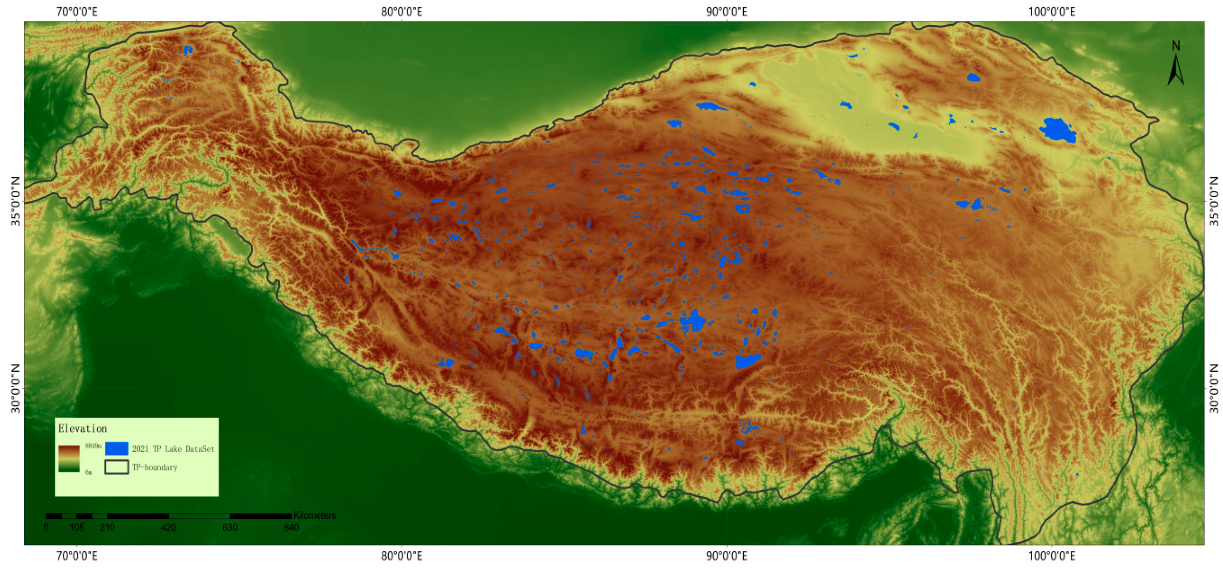
2.1. Research Region

This study region covers the entire Tibetan Plateau, and the administrative division covers the whole of Tibet, Qinghai, Xinjiang, Gansu, Sichuan, and Yunnan Provinces in China and parts of Nepal, Bhutan, India, Pakistan, Afghanistan, Tajikistan, and other countries. The total area is approximately 3.29374 million km², located at 25°48′51″ N–39°49′17″ N, 68°1′28″ E–104°41′7″ E. The longest distance from east to west is approximately 2800 km, the widest distance from north to south is approximately 1500 km [35], and the average elevation is more than 4000 m [36]. As shown in Figure 1, the topography of the Tibetan Plateau is complex, steep, and covered with mountains and rivers. Most of the mountains run east to west, except for the Hengduan Mountains in the southeast, which run north to south. These mountains and their parallel canyons and basins constitute the geomorphological framework of the Tibetan Plateau [35,37].

2.2. Data Sources

2.2.1. Landsat Image Data

Landsat 8 synthetic images of the Tibetan Plateau from 2016 and 2021 were used in this study. The source data were Landsat 8 atmospheric top layer (TOA) reflectance images. This dataset, with a spatial resolution of 30 m and temporal resolution of 16 d, was archived on the GEE cloud platform. The format is ee.ImageCollection (“LANDSAT/LC08/C02/T1_TOA”). The geo-reference accuracy of the image was better than 0.4 pixels [38].

2.2.2. DEM Data

The digital elevation data (DEM) were used to assist lake extraction from the InSAR Shuttle Radar Topography Mission (SRTM) data products collected by the Space Shuttle Radar topography mission in 2000. The format is ee.Image(“USGS/SRTMGL1_ 003”). The spatial resolution of the SRTM dataset is 30 m. The advantages of this dataset are that it has free access and strong realistic characteristics [39].

2.2.3. Regional Boundary Range Data

The Tibetan Plateau boundary vector dataset used in this study was obtained from the National Qinghai-Tibet Plateau Scientific Data Center (TPDC). The dataset is based on the SRTM data and is analyzed and produced with reference to some auxiliary data, in which the outer boundary of the study area is based on 2500 m contours [40].

2.2.4. Sampling and Verifying Data

For the extraction of lakes on the Tibetan Plateau in 2016 and 2021, four sample types including lakes, rivers and wetlands, ice and snow cover, and others were selected, and 1695 and 1568 samples were collected for each year, respectively (

Table 1. Type and quantity of sample points on the Tibetan Plateau.

2021		2016
Sample Categories	Number of Samples	Sample Categories	Number of Samples
Lake	684	Lake	455
River and wetland	200	River and wetland	471
Snow and ice cover	317	Snow and ice cover	400
Other	367	Other	369

).

All the sampling sites were used for supervised classification, of which 70% were used for training samples and 30% for verification samples.

To further validate the accuracy of lake extraction on the Tibetan Plateau, the classification was compared with the vector lake datasets of 2016 and 2021. The dataset was obtained from the HydroSHEDS global hydrological dataset and TPDC. The vector lake dataset in 2016 is tailored from the HydroLAKES global lake dataset included in HydroSHEDS, covering all lakes with a surface area equal to or more than 10 hectares (0.1 km²) on the earth’s surface [41]. The vector lake dataset of 2021 was developed by downloading the “larger than 1 km² Lake dataset in Tibetan Plateau (V3.0)” available on the official website of the TPDC. In this dataset, the observation data of 15 lakes from the entire Tibetan Plateau over the last 50 years (1970s–2021) were obtained using long time series Landsat remote sensing data, and changes in the number and area of lakes larger than 1 km² were analyzed in detail [22,42].

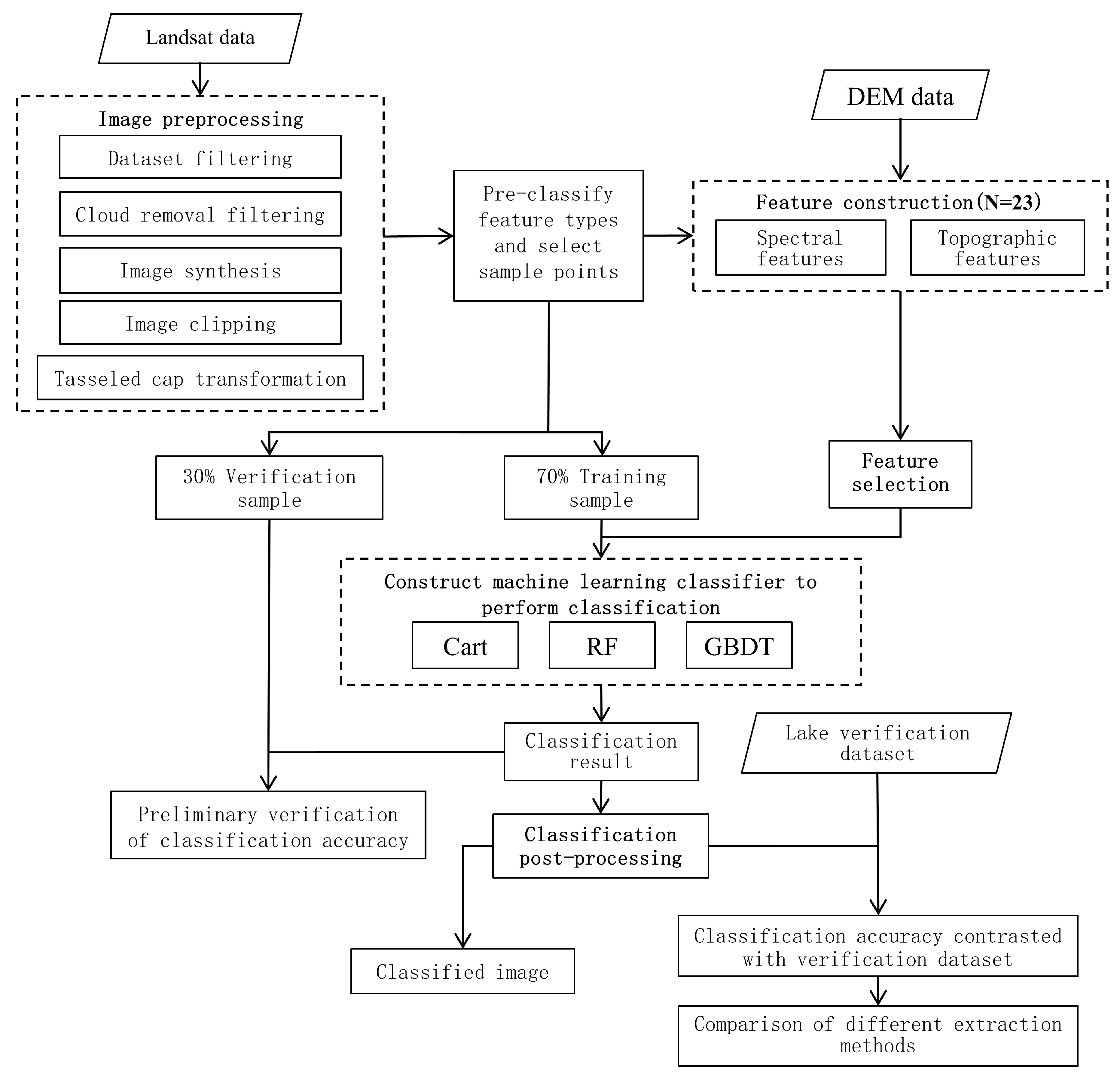
3. Flow Chart of Automatic Lake Extraction Method on the Tibetan Plateau

The lake extraction method includes six steps: image preprocessing, feature construction, feature selection, supervised classification, classification post-processing, and accuracy evaluation (Figure 2).

3.1. Image Preprocessing

The purpose of image preprocessing is to remove the influence of clouds and seasonal snowfall and synthesize the images in the study area of the Tibetan Plateau with less cloud and less snow. It includes five main steps: dataset filtering, cloud removal filtering, image synthesis, image clipping, and tasseled cap transformation. Dataset screening mainly establishes the research dataset according to the geographical scope and time of the study, and corresponds to the lake verification datasets. This study primarily used image datasets from 2016 and 2021. Cloud removal filtering uses the cloud scoring algorithm provided by the GEE platform, with scores ranging from 0 (no clouds) to 100 (very thick clouds) [23]. After repeated experiments, the optimal cloud-removal filter threshold obtained in this study was 25%. Image synthesis was orthorectified in GEE, and the overlapping data at each pixel position formed a pixel set. The median value of the pixel set was used to synthesize the image [24,25,26], that is, the median value of the sum of overlapping pixel values after cloud filtering of each pixel was used as the new pixel value to synthesize the complete image of the study area. Image clipping uses the “.clip()” function to call the Tibetan Plateau Boundary range data (TP-boundary) to crop the whole image to the area where only the study area is left [40]. The tasseled cap transform is a special principal component analysis method that compresses spectral data into several bands related to physical background features to reduce feature dimensions and enhance the effect of displaying image vegetation and water information [27]. The tasseled cap transformation converts the readings in a set of channels into composite values by using the weighted sum of the readings of each channel. In this study, after image cropping, tasseled cap transformation was used to obtain information about brightness, greenness, and wetness, which were used as feature vectors because they usually account for the greatest variation in a single-date image [28].

3.2. Feature Construction

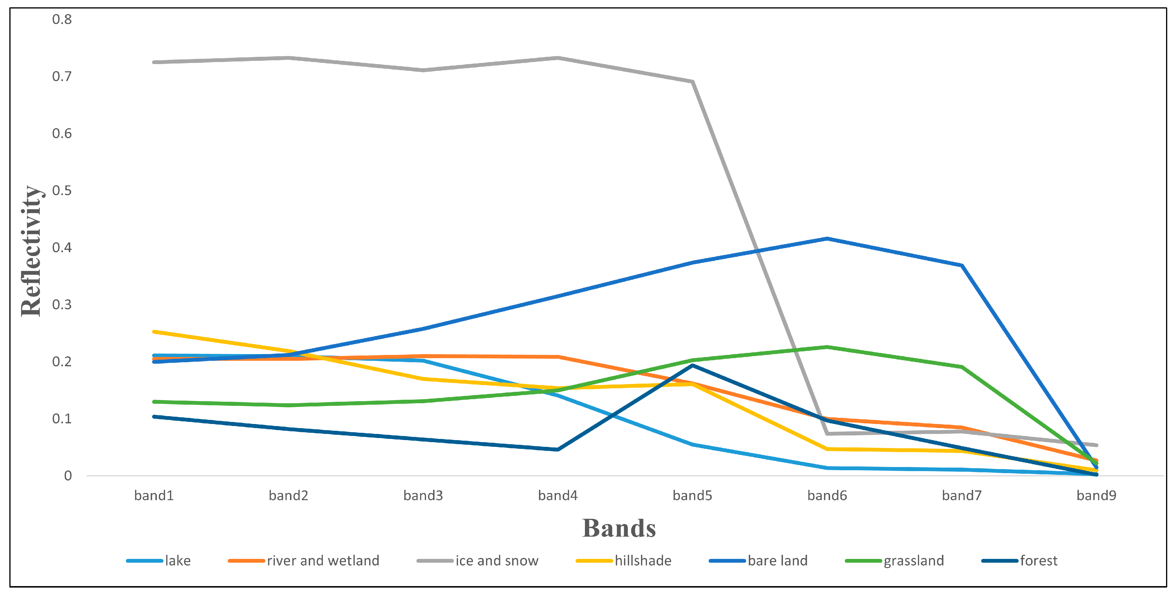
3.2.1. Spectral Characteristics

The characteristics of the water body reflected in each segment of the electromagnetic wave spectrum form the basis of water-body extraction from remote sensing images [43]. Researching spectral characteristic curves not only helps us to analysis the spectral reflection law of water body and other surface feature types, but also helps us to find the band combination with maximum spectral reflection difference between a water body and other surface objects. In this study, a certain number of sample points were randomly collected from lakes, rivers, wetlands, ice and snow, mountain shadows, bare lands, grasslands, forests, and other typical features on the Tibetan Plateau. The spectral reflectance values of the sample points in Band1–Band7 and Band9 were counted one by one, mean values of various ground objects in Band1–Band7 and Band9 were calculated, and spectral characteristic curves of typical features on the Tibetan Plateau were drawn (Figure 3).

Figure 3 shows that the reflectivity of lakes is generally low and mainly concentrated in the visible band, and the reflectivity of the band shows a significant attenuation trend, gradually approaching zero [44]. Additionally, only the spectral reflectance of lakes significantly decreases between Band4 and Band5; the spectral reflectance of other ground objects is larger than that of lakes between Band5 and Band, and does not gradually approach zero. For example, the spectral reflectance peaks of bare land, grassland, and forest appear in Band5 or Band6. Based on this, a new water body index is proposed in this study, which is the difference (RNSS) between the spectral reflectance of the red band and the sum of the spectral reflectance of the near infrared band, shortwave infrared Band1, and shortwave infrared Band2 of the Lansat8 OLI sensor, respectively. The calculation of the RNSS index is shown in Formula (8). We construct its calculation form based on the principle of band differential value. After the calculation of this form of band combination, the spectral reflection difference between the water-body pixels and other ground-object pixels increased. Therefore, this index can not only distinguish objects with different spectral characteristics but also increase the contrast of ground objects with similar spectral curves, such as mountains, rivers, and wetlands [44,45].

The spectral features used in this study also include the first band to the seventh band of the Landsat 8 OLI sensor called “Coastal”, “Blue”, “Green”, “Red”, “NIR”, “SWIR1”, and “SWIR2”, respectively. Besides these, there is a ninth band, “Cirrus,” whose wavelength range is 1.36–1.39 µm. This range is between the fifth and sixth bands and can compensate for the gap between these two bands. Additionally, the accuracy of lake extraction can be improved by introducing three characteristic components with physical meaning, namely, brightness, greenness and wetness, which are produced by the tasseled cap transformation. For this reason, eight types of spectral characteristic indexes were constructed based on the first to seventh bands of the sensor. The NDWI [11], MNDWI [12], enhanced water index (EWI) [46], NWI [14], revised normalized water index (RNDWI) [47], water index based on the fifth and sixth bands (NDWI₃) [28], automatic water extraction index (AWEI_nsh) [15], and RNSS water-body index were proposed in this study.

$$\mathrm{NDWI}=\frac{{\mathsf{\rho }}_{\mathrm{Green}}–{\mathsf{\rho }}_{\mathrm{NIR}}}{{\mathsf{\rho }}_{\mathrm{Green}}+{\mathsf{\rho }}_{\mathrm{NIR}}},$$

(1)

$$\mathrm{MNDWI}=\frac{{\mathsf{\rho }}_{\mathrm{Green}}–{\mathsf{\rho }}_{\mathrm{SWIR}1}}{{\mathsf{\rho }}_{\mathrm{Green}}+{\mathsf{\rho }}_{\mathrm{SWIR}1}},$$

(2)

$$\mathrm{EWI}=\frac{{\mathsf{\rho }}_{\mathrm{Green}}–{\mathsf{\rho }}_{\mathrm{NIR}}–{\mathsf{\rho }}_{\mathrm{SWIR}1}}{{\mathsf{\rho }}_{\mathrm{Green}}+{\mathsf{\rho }}_{\mathrm{NIR}}+{\mathsf{\rho }}_{\mathrm{SWIR}1}},$$

(3)

$$\mathrm{NWI}=\frac{{\mathsf{\rho }}_{\mathrm{Blue}}–{\mathsf{\rho }}_{\mathrm{NIR}}–{\mathsf{\rho }}_{\mathrm{SWIR}1}-{\mathsf{\rho }}_{\mathrm{SWIR}2}}{{\mathsf{\rho }}_{\mathrm{Blue}}+{\mathsf{\rho }}_{\mathrm{NIR}}+{\mathsf{\rho }}_{\mathrm{SWIR}1}+{\mathsf{\rho }}_{\mathrm{SWIR}2}}\times 10,$$

(4)

$$\mathrm{RNDWI}=\frac{{\mathsf{\rho }}_{\mathrm{SWIR}1}–{\mathsf{\rho }}_{\mathrm{Red}}}{{\mathsf{\rho }}_{\mathrm{SWIR}1}+{\mathsf{\rho }}_{\mathrm{Red}}},$$

(5)

$${\mathrm{NDWI}}_3=\frac{{\mathsf{\rho }}_{\mathrm{NIR}}–{\mathsf{\rho }}_{\mathrm{SWIR}1}}{{\mathsf{\rho }}_{\mathrm{NIR}}+{\mathsf{\rho }}_{\mathrm{SWIR}1}},$$

(6)

$${\mathrm{AWEI}}_{\mathrm{nsh}}=4\times \left({\mathsf{\rho }}_{\mathrm{Green}}-{\mathsf{\rho }}_{\mathrm{SWIR}1}\right)-0.25\times {\mathsf{\rho }}_{\mathrm{NIR}}+2.75\times {\mathsf{\rho }}_{\mathrm{SWIR}2},$$

(7)

$$\mathrm{RNSS}={\mathsf{\rho }}_{\mathrm{Red}}-{\mathsf{\rho }}_{\mathrm{NIR}}-{\mathsf{\rho }}_{\mathrm{SWIR}1}-{\mathsf{\rho }}_{\mathrm{SWIR}2},$$

(8)

In the form, ${\mathsf{\rho }}_{\mathrm{Blue}},{\mathsf{\rho }}_{\mathrm{Green}},{\mathsf{\rho }}_{\mathrm{Red}},{\mathsf{\rho }}_{\mathrm{NIR}},{\mathsf{\rho }}_{\mathrm{SWIR}1},{\mathsf{\rho }}_{\mathrm{SWIR}2}$ are the spectral reflectance values of the blue band, green band, red band, near infrared band, shortwave infrared Band1, and shortwave infrared Band2 of the Landsat 8 OLI sensor, respectively.

3.2.2. Topographic Features

The extraction of lakes relying only on spectral features is not ideal, and misclassification and omission can easily occur among the various types of ground features. The comprehensive use of various types of features for classification can, to a certain extent, reduce the influence of “different spectrum of the same body” and “the same spectrum of foreign body” effects on the classification and interaction between spectral features and effectively avoid the “pepper and salt phenomenon” [48]. In this study, the DEM data were used to construct four features as the input variables for the extraction method: elevation (Elevation), mountain shadow (Hillshade), slope (Slope), and slope aspect (Aspect). The topographic features are calculated using the “ee.Terrain.products ()” function and participate in the construction of the original features as four independent bands [49].

Table 2. Characteristic Indexes of Lake extraction in the Tibetan Plateau.

Characteristic Types	Source	Name
Spectral characteristics	Raw bands of sensor	B1-B7, B9
	Tasseled cap transformation of composite image	Brightness, Greenness, Wetness
	Combination of sensor raw bands	NDWI, MNDWI, EWI, NWI, RNDWI, NDWI3, AWEInsh, RNSS
Topographic characteristics	SRTMGL1_003	Elevation, Hillshade, Slope, Aspect

lists all the 23 features constructed in this study.

3.3. Feature Optimization

Selecting important features for image feature classification not only reduces the complexity of operation and improves the speed of operation, but also avoids the problem of dimensionality, which impacts feature optimization [50,51,52,53]. The GEE cloud platform provides feature importance analysis methods. The “.explain()” function in the classifier can calculate the importance information of each classification feature and quickly measure the importance weight of each feature indicator. In this study, we first calculated the importance scores of all the feature indicators, sorted them according to the importance scores from large to small, inputted the classifier for classification in turn, and finally selected the feature combination with the highest accuracy in the lake extraction model.

3.4. Supervised Classification

3.4.1. Classifier and Parameter Setting

The cart-type decision tree (Cart) [32], random forest (RF) [33], and gradient boosting decision tree (GBDT) [34] are all algorithm models based on decision trees, so it is convenient to control variables during comparison, and many feature indicators could be selected and added into these three classifiers. Among them, Cart is a decision tree that is optimized based on ID3. As a classification tree, the GINI value is used as the basis for node splitting [32]. However, the cart decision tree belongs to a single classifier, which is prone to overfitting, and there are limitations in processing large and complex datasets. Therefore, two representative decision-tree-based integrated learning algorithms, random forest (RF) and gradient boosting decision tree (GBDT), should be implemented [54]. These two algorithms comprise multiple decision trees but they are different because the RF uses the bagging idea in machine learning, whereas the GBDT uses the boosting idea [55,56].

The construction of classifier models requires several parameters, the most significant of which is the number of decision trees (N). In general, too small a value of N tends to cause under-fitting, whereas too large a value may cause memory overflow. In our study, the number of decision trees is chosen to be 10, and the other parameters are taken as default values [57].

3.4.2. Sample Selection

Sample selection was required for supervised classification. In this study, the entire study area was divided into four types: lakes, rivers and wetlands, snow cover, and others. The alluvial deposits and shoals on the image are classified as river and wetland to reduce the probability that the computer automatically classifies them into lakes. In the process of selecting all kinds of sample points, in line with the principle of random and uniform sampling, we attempt to cover the entire study area when collecting.

3.5. Classification Post-Processing

A common problem of pixel-based classification is that a few small spots are inevitably produced in the classification results which affect the quality and accuracy of the image [58]. Therefore, these small spots must be removed or reclassified [59]. In this study, the “updateMask” function was used to filter out the small patches with less than 200 adjacent pixels. The updateMask function masks the area with an image mask of 0 and retains the area with an image mask of 1. Then the “open” operation in the morphological change is used; its step is to etch the image first and then expand it, and its purpose is to eliminate the small patches, separate the features in the slender places, and smoothen the larger boundaries [31]. In the parameter setting of the open operation, the kernel radius of the morphological operator was set as 0.7, and the number of iterations was set as two.

3.6. Cartographic Accuracy Evaluation

In this study, accuracy verification metrics based on the classification confusion matrix, including overall accuracy, Kappa coefficient, producer’s accuracy, and user’s accuracy, were used to evaluate the accuracy of lake extraction. These four are the most commonly used metrics for testing classification results using validation samples [60]. The overall accuracy is the ratio of the sum of correctly classified pixels to the total number of pixels; user’s accuracy is the ratio of pixels correctly classified as this category to all pixels classified into this category; producer’s accuracy is the ratio of pixels correctly classified as this category to all ground true reference pixels of this category, and the Kappa coefficient is an indicator of the consistency test, which measures the classification effect. Its calculation formula is as follows:

$$\mathrm{Kappa}=\frac{{\mathrm{P}}_0-{\mathrm{P}}_{\mathrm{e}}}{1-{\mathrm{P}}_{\mathrm{e}}},$$

(9)

In this formula, P₀ is the overall accuracy, and Pe is the ratio of the sum of “product of classified and real pixel number” to “square of total samples” corresponding to all categories.

4. Results and Analysis

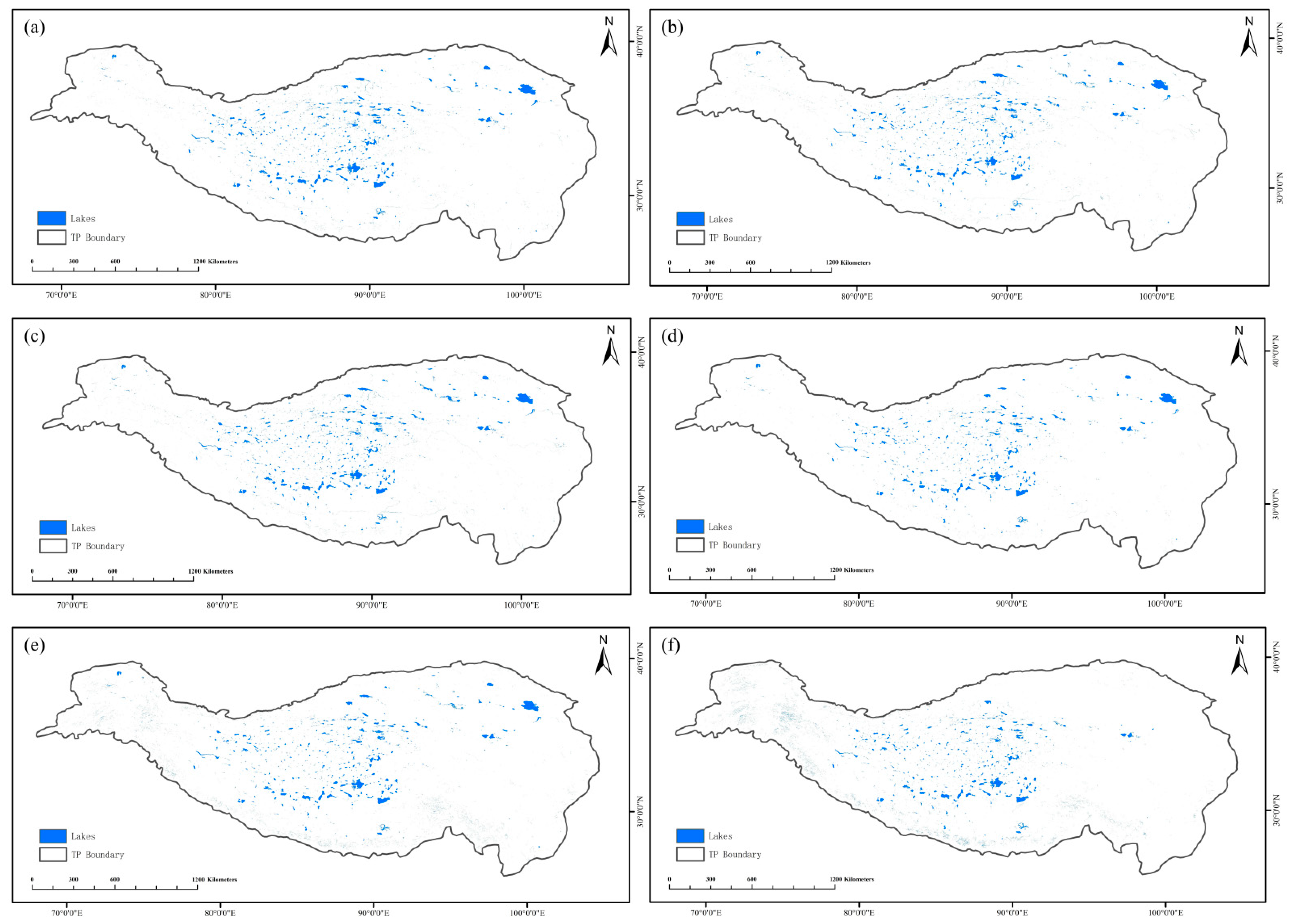
4.1. Automatic Lake Extraction of the Tibetan Plateau

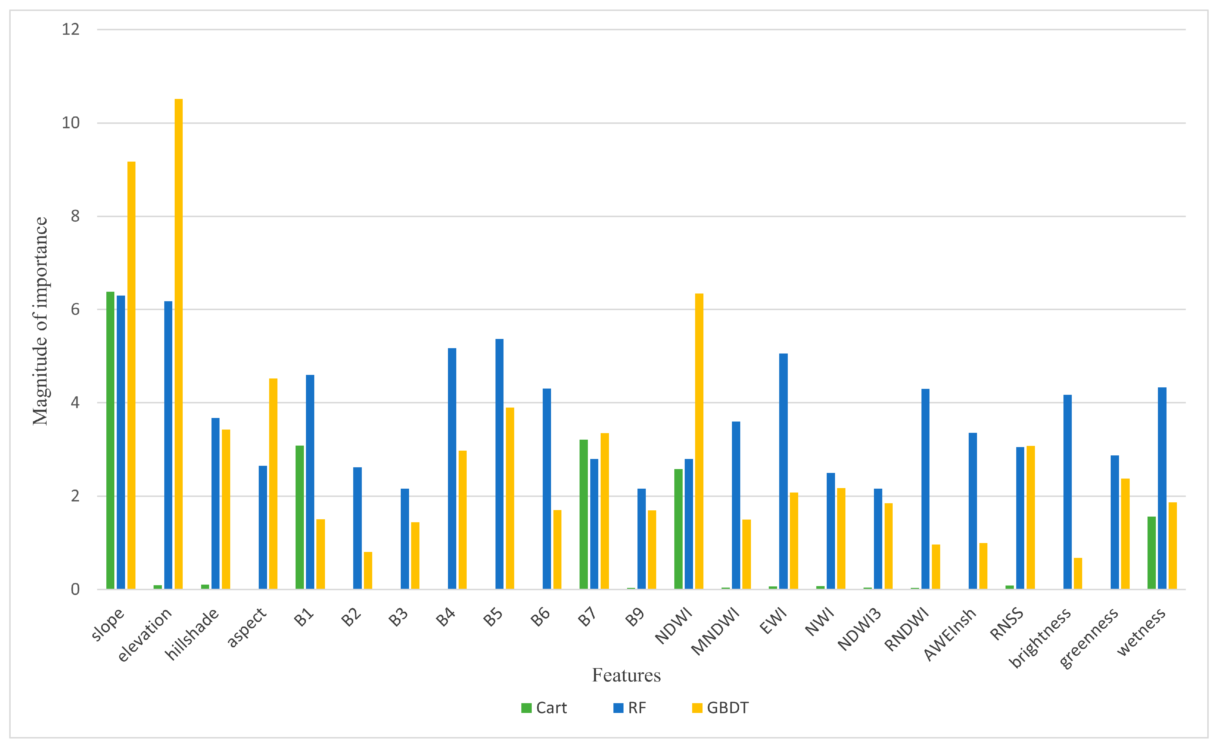
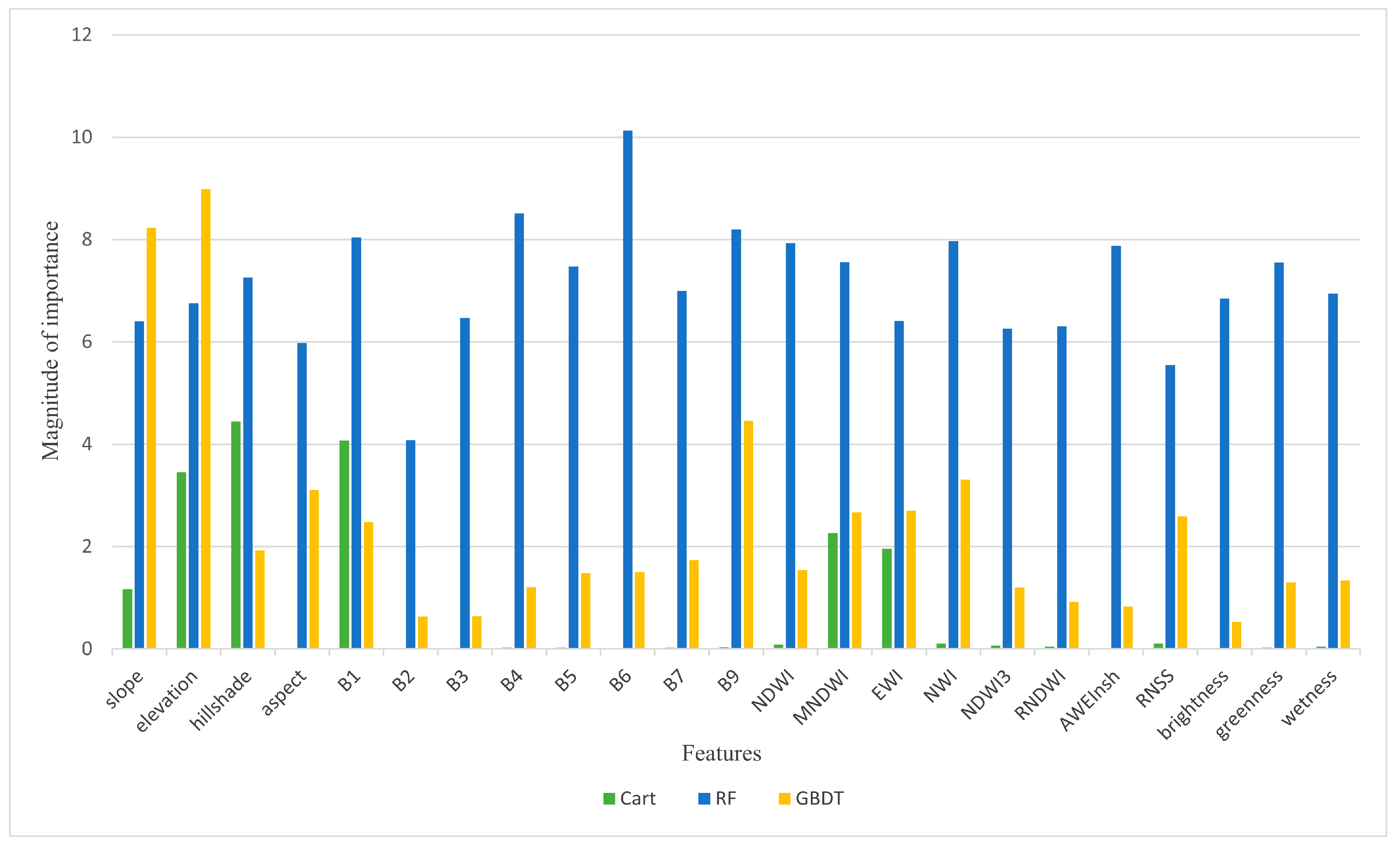
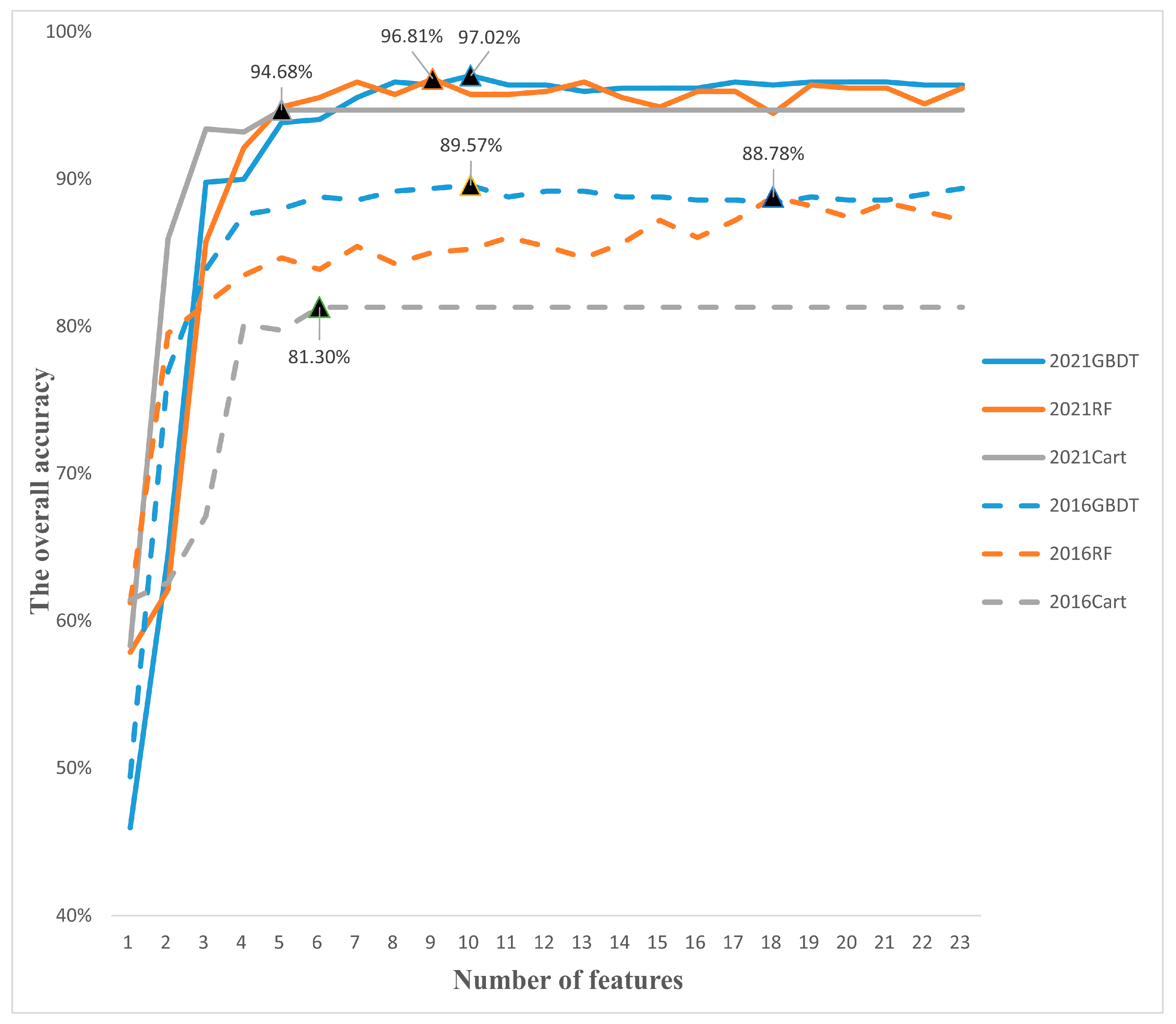
4.1.1. Feature Selection of Lake Extraction

Based on the 23 spectral and topographic features we constructed, together with the feature importance analysis method provided by the GEE cloud platform, this study calculated the importance scores of the 23 feature vectors in the Cart, RF, and GBDT classification algorithms of the 2016 and 2021 lake extraction (Figure 4 and Figure 5). The scores were used to indicate the magnitude of importance. The greater the importance, the higher the score. The importance values were standardized.

The features were sorted according to their importance scores, and the features with higher importance scores were individually selected in the GEE for classification. It was found that the RNSS lake extraction index constructed by band combination was of higher importance in both the Cart and GBDT classification methods. In this study, the top n (n∈[1, 23]) features with the highest importance scores in 2016 and 2021 were selected for classification, and the classification accuracy was individually calculated (Figure 6).

As shown in Figure 6, in the lake classification in 2021, the GBDT classification has the highest overall accuracy of 97.02% when considering the top ten features of importance. The RF classification of the overall accuracy of the model, which is 96.81%, is the highest when considering the top nine features of importance. In the Cart classification, the overall accuracy of the model, which is 94.68%, is the highest when considering the top five features of importance. In the lake classification in 2016, the GBDT classification has the highest overall accuracy of 89.57% when considering the top ten features of importance. In the RF classification, the overall accuracy of the model, which is 88.78%, is the highest when considering the top eighteen features of importance. In the Cart classification, the overall accuracy of the model is the highest, at 81.30%, when considering the top six features of importance. Additionally, in the Cart classification, only the most important features exert the most influence, and the contribution of other features has an order of magnitude gap from that of previous features and gradually tends to zero. Therefore, after the model accuracy reaches its peak, it becomes flat and can be regarded as unchanged.

Due to different natural conditions, ground truth, classification methods and sampling points of the study area each year, the feature importance and its order all have statistical differences. Additionally, after reaching the peak, the classification accuracy of all classification methods becomes flat or decreases to varying degrees, and there is no increase (Figure 6). Considering that increasing the number of features increases the computational complexity of the experiment, this study selects several features that participate in the classification when the accuracy reaches the peak in the classification feature analysis for lake extraction to ensure the accuracy and efficiency of classification (

Table 3. Extraction feature selection of the Tibetan Plateau lakes with different classification methods in each year.

Year	Classification Algorithm	Spectral Features	Topographic Features
2021	Cart	B1, B7, NDWI, Wetness	Slope
	RF	B1, B4, B5, B6, EWI, RNDWI, Wetness	Slope, Elevation
	GBDT	B4, B5, B7, NDWI, RNSS, Greenness	Elevation, Slope, Aspect, Hillshade
2016	Cart	B1, MNDWI, EWI	Hillshade, Elevation, Slope
	RF	B1, B3, B4, B5, B6, B7, B9, Greenness, Wetness, Brightness, NWI, NDWI, AWEInsh, MNDWI, EWI	Hillshade, Elevation, Slope
	GBDT	B1, B9, NWI, EWI, MNDWI, RNSS	Elevation, Slope, Aspect, Hillshade

).

4.1.2. Lake Extraction

The lakes on the Tibetan Plateau extracted using the Cart, RF, and GBDT classification methods in 2021 and 2016 are shown in Figure 7.

As the purpose of the preliminary accuracy verification is to determine the best feature combination involved in the classification, the actual classification effects of different classification methods must be compared with the lake verification datasets.

Table 4. Preliminary accuracy verification of the extraction results of lakes on the Tibetan Plateau by different classification methods.

Year	Classification Algorithm	Overall Accuracy	Kappa Coefficient	User’s Accuracy	Producer’s Accuracy
2021	GBDT	97.02%	0.958	98.18%	87.10%
	RF	96.81%	0.954	96.23%	82.26%
	Cart	94.68%	0.924	94.00%	75.81%
2016	GBDT	89.57%	0.861	85.71%	83.21%
	RF	88.78%	0.850	89.74%	76.64%
	Cart	81.30%	0.751	70.90%	69.34%

shows the preliminary accuracy verification of the different classification methods for the extraction results of lakes on the Tibetan Plateau.

4.2. Comparison of Lake Extraction from Different Machine Learning Methods

4.2.1. Verification Based on Vector Lake Datasets

To further confirm the actual classification effect of Cart, RF, and GBDT, the classification results were compared with the vector lake datasets for 2016 and 2021, as shown in

Table 5. The accuracy of comparisons between the extraction results of lakes on the Tibetan Plateau and verified datasets.

Year	Classification Algorithm	Overall Accuracy	Kappa Coefficient	User’s Accuracy	Producer’s Accuracy
2021	GBDT	99.88%	0.933	89.18%	98.24%
	RF	99.86%	0.929	89.01%	97.27%
	Cart	99.84%	0.919	86.52%	95.89%
2016	GBDT	99.81%	0.887	83.55%	94.67%
	RF	99.67%	0.815	72.36%	93.70%
	Cart	99.43%	0.650	61.58%	69.54%

.

The GBDT classification method constructed in this study performs best in the information extraction of lakes on the Tibetan Plateau, and its four accuracy metrics are the highest. The RF classification method takes the second place, whereas the Cart classification method is the worst. The Kappa coefficient, user’s accuracy, and producer’s accuracy of the Cart classification for lake extraction in 2016 do not reach the experimental standard (more than 70%), and there is a wide range of omissions. This study further compares the extraction accuracy of the three classification methods from the extracted total lake area (

Table 6. Comparison of extracted area and validation datasets of lakes on the Tibetan Plateau.

Year	Project	Total Lake Area (km2)	Error Proportion
2021	Validation dataset	61333.31	/
	Extraction of GBDT	65949.28	7.53%
	Extraction of RF	67029.99	9.29%
	Extraction of Cart	69640.28	13.54%
2016	Validation dataset	49330.02	/
	Extraction of GBDT	55892.53	13.30%
	Extraction of RF	63876.03	29.49%
	Extraction of Cart	55708.78	12.93%

) and uses the absolute percentage error formula to calculate the proportion of extraction error of the total lake area after contrasting with validation datasets. The magnitude of the absolute percentage error is defined as: |(extracted validation)/validation| × 100% [61].

The three classification methods all have different degrees of over-extraction of lakes on the Tibetan Plateau, which is related to the small area spots generated by pixel classification [58]. Although masking and morphological operations were performed during the study, this problem persisted. In 2016, the total area of lakes extracted by the Cart classification method was low owing to the existence of large-scale omissions, which resulted in a low proportion of errors in the total area of lake extraction. In summary, the extraction result of the GBDT classification method is the closest to the verification dataset among the three classification methods, and can be used to extract lakes in the Tibetan Plateau.

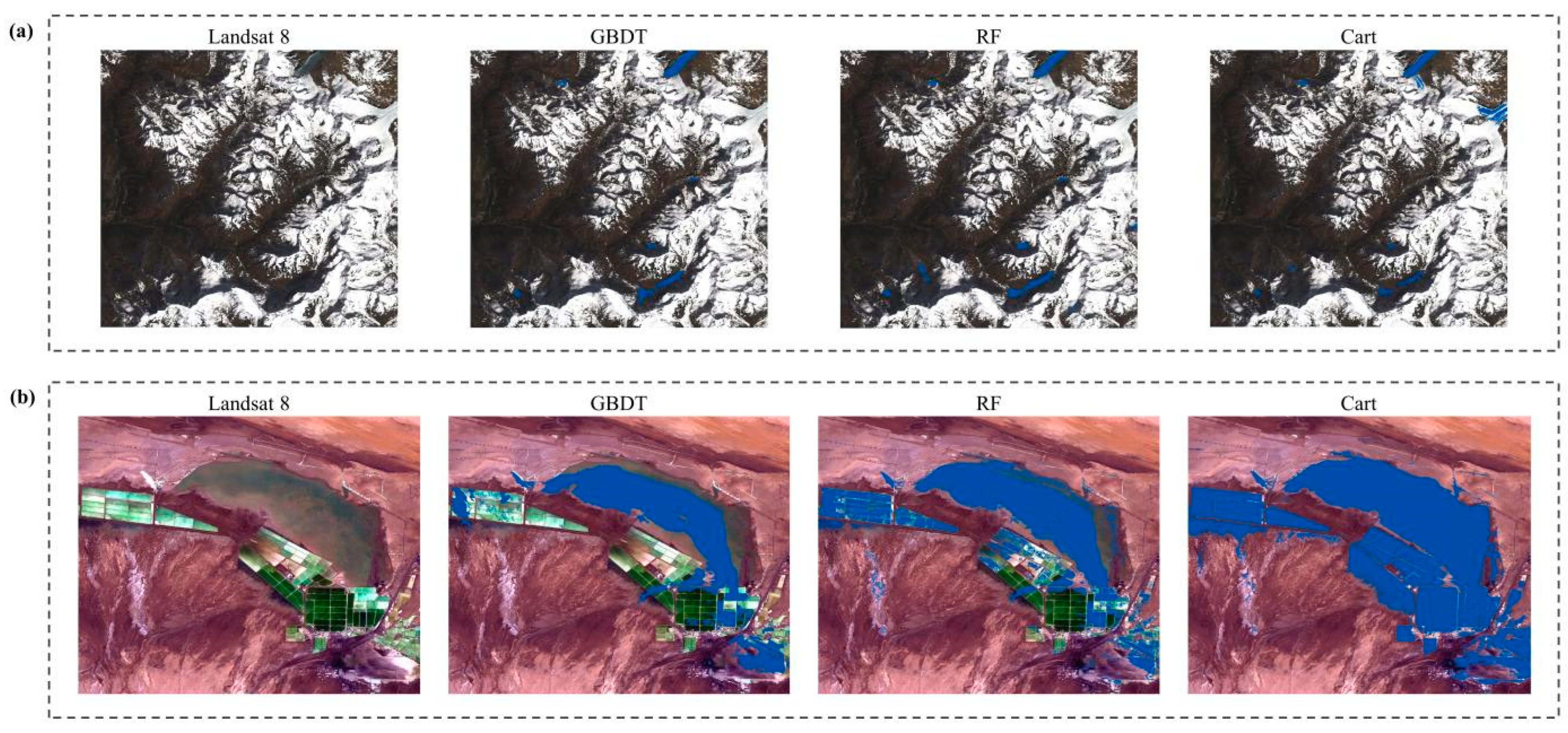
4.2.2. Key Areas Comparison of Lake Extraction

Both supervised classification and unsupervised classification methods cannot effectively identify glaciers in shadows [62], confusing them with lakes. Second, the types of features, such as alluvial deposits and shoals, also interfere with the extraction of lakes, and the areas with high water content are mistakenly extracted as lakes [6,46]. In this study, through cloud removal filtering and an annual median image synthesis operation, the interference of cloud content in the study area image on lake extraction can be effectively avoided, and the effects of cloud occlusion or areas with empty pixel values on the three classification methods are identical. Therefore, this study does not consider the influence of cloud occlusion on the three classification methods.

Figure 8 shows the detailed regional extraction results of the three classification methods under the influence of mountain shadow and snow cover (Figure 8a) and under the influence of similar features such as alluvium and shoals (Figure 8b). The base map of the regional detail was synthesized by the four, three, and two bands of the Landsat 8 OLI image, and lake water area extracted by the three classification methods is shown in blue. As can be seen from Figure 8a, the three classification methods mistakenly extract some mountain shadows into lakes; among them, the RF method has the most mistakenly extracted areas, followed by the GBDT and Cart methods. All three classification methods can extract the lakes covered with ice and snow, among which the GBDT classification method has the smallest extraction area. The RF classification method takes the second place. The Cart classification method has the largest extraction area; but it also mistakenly extracts a large range of ice and snow into lakes. As shown in Figure 8b, the boundary of the natural lake (East Dabusun Salt Lake) is located at the upper-right of the image, and the lower edge of the lake is adjacent to similar saline-alkali beaches or pond-like artificial features, which could not be classified as lakes when classifying the features. Therefore, it was selected as the river and wetland type in this study. Nevertheless, the three classification methods still had different degrees of misextraction. The range of lakes extracted by the GBDT classification method was the smallest and closest to the actual lake boundary range. The range of lakes mistakenly extracted by the RF classification method was larger; however, that extracted by the Cart classification method was the largest. In summary, although the area of lake water extracted by the GBDT classification method was small, the extraction accuracy was the highest. The real lake pixels accounted for a higher proportion of the pixels identified as lakes by the classifier and had higher user’s accuracy and overall accuracy.

5. Discussion

Numerous studies have shown that the overall classification effect of the machine learning lake extraction method based on multiple feature datasets is better than that of the traditional method of determining the lake extraction threshold based on a single feature index and manual experiments [6,16,51,63,64]. To evaluate the classification effect of machine learning lake extraction methods with multiple feature datasets, this study analyzed the four factors that affect the lake extraction accuracy of the Cart, RF, and GBDT classification methods, including feature and sample selection, DEM data accuracy, snow cover, and verification datasets.

5.1. Feature and Sample Selection

To select the best feature combination for classification, this study selected important features using the “.explain()” method, which improved the extraction accuracy of each classification method and reduced the false and missing extraction rates [53,65]. However, it could not maximize the efficiency of classification because there may have been a correlation between the selected features, which leads to information redundancy. Therefore, the selection of important and low-correlation features to maximize the efficiency of classification needs to be further studied.

In this study, visual interpretation was required for sample selection in the process of supervised classification, which could not avoid the interference of human subjective factors in the sampling process and was, therefore, affected by the complex natural environment of the Tibetan Plateau. It is impossible to ensure that all kinds of ground objects collected are completely accurate, comprehensive, and evenly distributed, which also affects the extraction accuracy of lakes [64]. Therefore, future research can use high-resolution remote sensing images (the Sentinel series or high-score series) for visual interpretation to enhance the accuracy of the classification results.

5.2. DEM Data Precision

The precision of the DEM data directly affected the topographic features used for lake extraction during the classification process of this study. The features of elevation, mountain shadow, slope, and aspect constructed in this study were all from the SRTMGL1_003 DEM data. However, the DEM data with 30 m resolution may not fully reflect the detailed features of topography and geomorphology, and the influence of mountain shadows persists [59]. Thus, more accurate DEM data could be used to solve this problem in future research.

5.3. Snow Cover

It was identified that when extracting lakes in alpine areas, it was difficult to remove the influence of permanent snow using only spectral and topographic features, especially for ice-covered lakes, which frequently led to confusion during extraction [59]; textural features can be used to solve this problem [66]. Therefore, the influence of textural features can be investigated in future lake extraction.

5.4. Validation Datasets

In addition to these factors, the accuracy of lake extraction on the Tibetan Plateau was affected by the validation datasets. The validation datasets only contained the natural boundary of lakes and did not include artificial features such as reservoirs, paddy fields, ponds, and saline-alkali beaches; these artificial features are likely to be mistakenly extracted as lakes. Although this study took corresponding measures to classify the types of objects and collect sample points, the problem of false extraction remains inevitable; therefore, shape feature-assisted extraction, such as shape index, can be considered in the future [67].

The above discusses the limitations and challenges of these extraction method procedures in terms of feature selection, sample collection, data accuracy, validation datasets, etc. Moreover, these methods have the disadvantages of complex procedures and non-optimal parameter settings. These factors require further optimization.

6. Conclusions

In this study, to reduce the influence of lake ice and snow cover, mountain shadows, cloud and fog shade, alluvium, and shoal on the extraction of Tibetan Plateau lakes, an RNSS water-body index was proposed to increase the contrast between lakes and features with similar spectral curves. Combined with the existing lake extraction feature indexes and machine learning classification algorithms, three automatic extraction methods were compared to determine the method with the best classification accuracy of the Tibetan Plateau lakes.

The effects of three machine learning classification methods on lake extraction were studied and compared, and the GBDT method was found to be the best. The results show that the four accuracy evaluation indexes of this method are the highest in the lake extraction of the Tibetan Plateau in 2016 and 2021, and the total lake area extracted is most consistent with the validation datasets. This method can not only accurately extract most of the lakes on the Tibetan Plateau but is also least affected by environmental factors. Additionally, it has the advantages of transferable time ranges and the capability to switch to different datasets. Compared with the traditional classification method based on determining the threshold of lake extraction by individual feature metrics or manual experiments, it has higher robustness and generalizability.

References

1. Lu, A.; Yao, T.; Wang, L. Remote sensing study on the changes of typical glaciers and lakes in Qinghai-Xizang Plateau. Glacial Permafr. 2005, 6, 783–792. [Google Scholar]
2. Lu, A.; Wang, L.; Yao, T. Study on remote sensing methods for modern changes of lakes in Qinghai-Xizang Plateau. Remote Sens. Technol. Appl. 2006, 3, 173–177. [Google Scholar]
3. Liu, B.; Li, L.; Du, Y.; Liang, T.; Duan, S.; Hou, F.; Ren, J. Analysis on the cause and influence of embankment collapse of Zhuonai Lake in Hoh Xili, Qinghai-Tibet Plateau. Glacial Permafr. 2016, 38, 305–311. [Google Scholar]
4. Sun, H. The Formation and Evolution of the Qinghai-Xizang Plateau; Shanghai Science and Technology Press: Shanghai, China, 1996. [Google Scholar]
5. Lv, L.; Zhang, T.; Yi, G.; Miao, J.; Li, J.; Bie, X.; Huang, X. Response relationship between lake area change and climatic factors in Qinghai-Xizang Plateau since 2000. Lake Sci. 2019, 31, 573–589. [Google Scholar]
6. Li, D.; Wu, B.; Chen, B.; Xue, Y.; Zhang, Y. Research progress and prospect of water information extraction based on satellite remote sensing. J. Tsinghua Univ. 2020, 60, 147–161. [Google Scholar]
7. Du, Y.; Zhou, C. Automatic extraction method of remote sensing information of water body. J. Remote Sens. 1998, 4, 264–269. [Google Scholar]
8. Su, L.; Li, Z.; Gao, F.; Yu, M. A review of water extraction from remote sensing images. Remote Sens. Land Resour. 2021, 33, 9–19. [Google Scholar]
9. Zhou, C.; Luo, J.; Yang, X. Geoscience Understanding and Analysis of Remote Sensing Images; Science Publishing House: Beijing, China, 1999. [Google Scholar]
10. Wang, J.; Zhang, Y.; Kong, G. Application of spectral relation method in water feature extraction. Mine Surv. 2004, 4, 30–32. [Google Scholar]
11. McFeeters, S.K. The use of the Normalized Difference Water Index (NDWI) in the delineation of open water features. Int. J. Remote Sens. 1996, 17, 1425–1432. [Google Scholar] [CrossRef]
12. Xu, H. Study on extracting water information using modified normalized difference water body index (MNDWI). J. Remote Sens. 2005, 5, 589–595. [Google Scholar]
13. Li, L.; Su, H.; Du, Q.; Wu, T. A novel surface water index using local background information for long term and large-scale Landsat images. ISPRS J. Photogramm. Remote Sens. 2021, 172, 59–78. [Google Scholar] [CrossRef]
14. Ding, F. Experimental study on water information extraction based on new water index (NWI). Sci. Surv. Mapp. 2009, 34, 155–157. [Google Scholar]
15. Feyisa, G.L.; Meilby, H.; Fensholt, R.; Proud, S.R. Automated Water Extraction Index: A new technique for surface water mapping using Landsat imagery. Remote Sens. Environ. 2014, 140, 23–35. [Google Scholar] [CrossRef]
16. Cui, Q.; Wang, J.; Wang, M. Vector constrained water extraction from object-oriented high-score remote sensing images. Remote Sens. Inf. 2018, 33, 115–121. [Google Scholar]
17. Li, M.; Hong, L.; Guo, J.; Zhu, A. Automated extraction of lake water bodies in complex geographical environments by fusing Sentinel-1/2 Data. Water 2022, 14, 30. [Google Scholar] [CrossRef]
18. Shen, L.; Li, C. Water body extraction from Landsat ETM+ imagery using Adaboost algorithm. In Proceedings of the 18th International Conference on Geoinformatics, Beijing, China, 18–20 June 2010; pp. 1–4. [Google Scholar] [CrossRef]
19. Ko, B.C.; Kim, H.H.; Nam, J.Y. Classification of Potential Water Bodies Using Landsat 8 OLI and a Combination of Two Boosted Random Forest Classifiers. Sensors 2015, 15, 13763–13777. [Google Scholar] [CrossRef] [Green Version]
20. Barbieux, K.; Charitsi, A.; Merminod, B. Icy lakes extraction and water-ice classification using Landsat 8 OLI multispectral data. Int. J. Remote Sens. 2018, 39, 3646–3678. [Google Scholar] [CrossRef]
21. Wang, Z.; Li, J.; Bao, A.; Zhang, J.; Bai, J. Temporal change and attribution of Balikun Lake area in Xinjiang from 1995 to 2020. Study Arid. Area 2021, 38, 1514–1523. [Google Scholar]
22. Zhang, G.; Yao, T.; Xie, H.; Zhang, K.; Zhu, F. Lakes’ state and abundance across the Tibetan Plateau. Chin. Sci. Bull. 2014, 59, 3010–3021. [Google Scholar] [CrossRef]
23. Huang, L.; Li, Z.; Zhou, J.; Zhang, P. An automatic method for clean glacier and nonseasonal snow area change estimation in High Mountain Asia from 1990 to 2018. Remote Sens. Environ. 2021, 258, 112376. [Google Scholar] [CrossRef]
24. Wang, Y.; Zhao, Y.; Wu, J. Long-term dynamic monitoring of ecological quality of urban agglomeration based on GoogleEarthEngine Cloud Computing—A case study of Guangdong-Hong Kong-Macau Greater Bay Area. J. Ecol. 2020, 40, 8461–8473. [Google Scholar]
25. Niu, Q.; Liu, L.; Huang, G.; Cheng, Q.; Cheng, Y. Identification of complex planting structure in Hetao Irrigation District based on GEE and machine learning. J. Agric. Eng. 2022, 38, 165–174. [Google Scholar]
26. Li, P.; Liu, X.; Huang, Y.; Zhang, H. Extraction of impervious water surface time series in main urban area of Guangzhou City based on GEE platform. J. Geo-Inf. Sci. 2020, 22, 638–648. [Google Scholar]
27. Crist, E.P.; Cicone, R.C. A Physically-Based Transformation of Thematic Mapper Data—The TM Tasseled Cap. IEEE Trans. Geosci. Remote Sens. 1984, 22, 256–263. [Google Scholar] [CrossRef]
28. Ouma, Y.O.; Tateishi, R. A water index for rapid mapping of shoreline changes of five East African rift valley lakes: An empirical analysis using Landsat TM and ETM+ data. Int. J. Remote Sens. 2006, 27, 3153–3181. [Google Scholar] [CrossRef]
29. Gorelick, N.; Hancher, M.; Dixon, M.; Ilyushchenko, S.; Thau, D.; Moore, R. Google Earth Engine: Planetary-scale geospatial analysis for everyone. Remote Sens. Environ. 2017, 202, 18–27. [Google Scholar] [CrossRef]
30. Hird, J.N.; Kariyeva, J.; Mcdermid, G.J. Satellite time series and Google Earth Engine democratize the process of forest—Recovery monitoring over large areas. Remote Sens. 2021, 13, 4745. [Google Scholar] [CrossRef]
31. Dong, J.; Li, S.; Zeng, Y.; Yan, K.; Fu, D. Remote Sensing Cloud Computing and Scientific Analysis—Application and Practice; Science Publishing House: Beijing, China, 2020. [Google Scholar]
32. Zhou, Z. Machine Learning; Tsinghua University Press: Beijing, China, 2016. [Google Scholar]
33. Breiman, L. Random forests. Mach. Learn. 2001, 45, 5–32. [Google Scholar] [CrossRef] [Green Version]
34. Jerome, H.F. Greedy function approximation: A gradient boosting machine. Ann. Stat. 2001, 29, 5. [Google Scholar]
35. Wang, Z. Multi-Source Remote Sensing Monitoring of Environmental Elements of Lakes in Qinghai-Xizang Plateau and Its Response to Climate Change. Master’s Thesis, Shandong Normal University, Jinan, China, 2017. [Google Scholar]
36. Bohner, J. General climatic controls and topoclimatic variations in Central and High Asia. Boreas 2006, 35, 279–295. [Google Scholar] [CrossRef]
37. Liang, D. Lake Area Change in Qinghai-Xizang Plateau and Its Response to Climate Change from 1975 to 2010. Master’s Thesis, China University of Geosciences, Beijing, China, 2016. [Google Scholar]
38. Chen, F.; Zhang, M.; Tian, B.; Li, Z. Extraction of Glacial Lake Outlines in Tibet Plateau Using Landsat 8 Imagery and Google Earth Engine. IEEE J. Sel. Top. Appl. Earth Obs. Remote Sens. 2017, 10, 4002–4009. [Google Scholar] [CrossRef]
39. Farr, T.G.; Rosen, P.A.; Caro, E.; Crippen, R.; Duren, R.; Hensley, S.; Kobrick, M.; Paller, M.; Rodriguez, E.; Roth, L.; et al. The shuttle radar topography mission. Rev. Geophys. 2007, 45, 2. [Google Scholar] [CrossRef] [Green Version]
40. Zhang, G.; Yao, T.; Xie, H.; Kang, S.; Lei, Y. Increased mass over the Tibetan Plateau: From lakes or glaciers? Geophys. Res. Lett. 2013, 40, 2125–2130. [Google Scholar] [CrossRef]
41. Messager, M.L.; Lehner, B.; Grill, G.; Nedeva, I.; Schmitt, O. Estimating the volume and age of water stored in global lakes using a geo-statistical approach. Nat. Commun. 2016, 7, 13603. [Google Scholar] [CrossRef]
42. Zhang, G.; Luo, W.; Chen, W.; Zheng, G. A robust but variable lake expansion on the Tibetan Plateau. Sci. Bull. 2019, 64, 1306–1309. [Google Scholar] [CrossRef]
43. Tan, Q.; Liu, Z.; Hu, J. Extraction of morphological parameters of Poyang Lake using multi-source remote sensing images. J. Beijing Jiaotong Univ. 2006, 30, 26–30. [Google Scholar]
44. Bi, H.; Wang, S.; Zeng, J.; Zhao, Y.; Wang, H.; Yin, H. Comparison and analysis of several common water extraction methods based on TM images. Remote Sensing Information 2012, 27, 77–82. [Google Scholar]
45. Chen, H.; Wang, J.; Chen, Z.; Yang, L.; Xi, W. Comparison of methods for extracting water body information from TM images in mountainous and plateau areas—Taking part of Shangri La County as an example. Remote Sens. Technol. Appl. 2004, 6, 479–484. [Google Scholar]
46. Yan, P.; Zhang, Y.; Zhang, Y. Study on extracting water system information in semi-arid area using enhanced water index (EWI) and GIS noise removal technology. Remote Sens. Inf. 2007, 6, 62–67. [Google Scholar]
47. Cao, R.; Li, C.; Liu, L.; Wang, J.; Yan, G. Miyun Reservoir area extraction and change monitoring based on water index. Sci. Surv. Mapp. 2008, 2, 158–160. [Google Scholar]
48. Wang, A.; Liu, J.; Wang, C.; Wang, R. Dongping Lake wetland information extraction based on density segmentation and object oriented. J. Shandong Agric. Univ. 2017, 48, 70–74. [Google Scholar]
49. Sazib, N.; Mladenova, I.; Bolten, J. Leveraging the Google Earth Engine for drought assessment using global soil moisture data. Remote Sens. 2018, 10, 1265. [Google Scholar] [CrossRef] [PubMed] [Green Version]
50. Kuo, F.Y.; Sloan, I.H. Lifting the curse of dimensionality. Not. AMS 2005, 52, 1320–1328. [Google Scholar]
51. Acharya, T.D.; Subedi, A.; Lee, D.H. Evaluation of Machine Learning Algorithms for Surface Water Extraction in a Landsat 8 Scene of Nepal. Sensors 2019, 19, 2769. [Google Scholar] [CrossRef] [Green Version]
52. Bach, F. Breaking the curse of dimensionality with convex neural networks. J. Mach. Learn. Res. 2017, 18, 629–681. [Google Scholar]
53. Zhang, X.; Feng, X.; Jiang, H. Feature space optimization of object-oriented classification. J. Remote Sens. 2009, 13, 664–677. [Google Scholar]
54. Chen, Y. Analysis and comparison of random forest and gradient lifting decision tree based on integrated learning algorithm. Comput. Knowl. Technol. 2021, 17, 32–34. [Google Scholar]
55. Breiman, L. Bagging predictors. Mach. Learn. 1996, 24, 123–140. [Google Scholar] [CrossRef] [Green Version]
56. Freund, Y.; Schapire, R.E. A Decision-Theoretic Generalization of On-Line Learning and an Application to Boosting. J. Comput. Syst. Sci. 1997, 55, 119–139. [Google Scholar] [CrossRef] [Green Version]
57. Gislason, P.O.; Benediktsson, J.A.; Sveinsson, J.R. Random Forests for land cover classification. Pattern Recognit. Lett. 2006, 27, 294–300. [Google Scholar] [CrossRef]
58. Huang, X.; Lu, Q.; Zhang, L.; Plaza, A. New Postprocessing Methods for Remote Sensing Image Classification: A Systematic Study. IEEE Trans. Geosci. Remote Sens. 2014, 52, 7140–7159. [Google Scholar] [CrossRef]
59. Hu, M.; Zhou, G.; Lv, X.; Zhou, L.; He, X.; Tian, Z. A new automatic extraction method for glaciers on the Tibetan Plateau under clouds, shadows and snow cover. Remote Sens. 2022, 14, 3084. [Google Scholar] [CrossRef]
60. Zourarakis, D.P. Remote Sensing Handbook—Volume I: Remotely Sensed Data Characterization, Classification, and Accuracies. Photogramm. Eng. Remote Sens. 2018, 84, 481. [Google Scholar] [CrossRef]
61. Tofallis, C. Measuring relative accuracy: A better alternative to mean absolute percentage error. SSRN Electronic Journal. 2013. [Google Scholar] [CrossRef]
62. Ji, X.; Chen, Y.; Luo, X.; Li, Y. Study on the identification method of glacier in mountain shadows based on Landsat 8 OLI image. Spectrosc. Spectr. Anal. 2018, 38, 3857–3863. [Google Scholar]
63. Zhang, H.; Wang, D.; Gao, Y.; Gong, W. Research on information extraction of shaded water body based on OLI data and decision tree method. Surv. Mapp. Eng. 2017, 26, 45–48. [Google Scholar]
64. Sun, J. Surface Water Information Extraction from High Resolution Remote Sensing Images Based on Ensemble Learning. Master’s Thesis, Jilin University, Changchun, China, 2020. [Google Scholar]
65. Cui, Q.; Wang, M.; Huang, Y. Extraction of water information in Shanghai based on random forest model and six kinds of water index. Bull. Surv. Mapp. 2022, 2, 106–109. [Google Scholar]
66. Rajesh, K.; Jawahar, C.V.; Sengupta, S.; Sinha, S. Performance analysis of textural features for characterization and classification of SAR images. Int. J. Remote Sens. 2001, 22, 1555–1569. [Google Scholar] [CrossRef]
67. Du, J.; Huang, Y.; Feng, X.; Wang, Z. Research on water extraction and classification from SPOT satellite images. J. Remote Sens. 2001, 3, 214–219. [Google Scholar]
Figure 1. Schematic diagram of the study area. The base map is from the digital elevation data produced by The Shuttle Radar Topography Mission (SRTM). The TP Lake DataSet and TP boundary are vector datasets obtained by the National Tibetan Plateau Scientific Data Center.
Remotesensing 15 00267 g001
Figure 2. Lake extraction flow chart.
Remotesensing 15 00267 g002
Figure 3. Spectral characteristic curves of typical features on the Tibetan Plateau.
Remotesensing 15 00267 g003
Figure 4. The importance of extracting features of lakes on the Tibetan Plateau in 2021.
Remotesensing 15 00267 g004
Figure 5. The importance of extracting features of lakes on the Tibetan Plateau in 2016.
Remotesensing 15 00267 g005
Figure 6. Classification feature analysis based on different classifications.
Remotesensing 15 00267 g006
Figure 7. The distribution of lakes on the Tibetan Plateau extracted by different classification methods and characteristic indexes: (a) GBDT extraction maps in 2021, (b) RF extraction maps in 2021, (c) Cart extraction maps in 2021, (d) GBDT extraction maps in 2016, (e) RF extraction maps in 2016, and (f) Cart extraction maps in 2016.
Remotesensing 15 00267 g007
Figure 8. The detailed extraction results of the three classification methods in the difficult areas of lake extraction on the Tibetan Plateau. Among them, (a) is the extraction result under the influence of mountain shadow and ice and snow cover, and (b) is the extraction result under the influence of similar features such as alluvial deposits and shoals.
Remotesensing 15 00267 g008