Mapping of Greenhouse Gas Concentration in Peninsular Malaysia Industrial Areas Using Unmanned Aerial Vehicle-Based Sniffer Sensor

Abstract

The increasing concentration of greenhouse gas (GHG) emissions due to increased fossil fuel consumption for manufacturing activities to support population growth is worrisome. Carbon dioxide (CO₂) and methane (CH₄) remain the two GHGs that contribute to the impact of global warming, and inventorying their concentrations is important for monitoring their changes, which can be used to infer their emissions over time. Hence, this article highlights sniffer4D, an unmanned aerial vehicle (UAV)-based air pollutant mapping system that visualise and analyse three-dimensional (3D) air pollution data in real time, for mapping GHGs concentrations within industrial areas. Consequently, GHGs concentrations for two industrial and adjacent residential areas in Johor, Peninsular Malaysia were mapped. The GHGs concentrations were validated using a ground-based portable gas detector. The results revealed that CO₂ has the highest concentration mean of 625.235 mg/m³, followed by CH₄ with a mean of 249.239 mg/m³. The mapped UAV GHG concentration also reported good agreement with the in situ observations with an RMSE of 7 and 6 mg/m³ for CO² and CH₄ concentration, respectively. Ozone and nitrogen dioxide mixture (O₃ + NO₂) with a mean concentration of 249 μg/m³ and an RMSE of 9 μg/m³ are the remaining significant concentrations reported. This approach shall assist in fast-tracking the United Nations climate change mitigation agenda.

1. Introduction

Although greenhouse gases (GHGs) are said to have a modulating effect on the Earth’s atmosphere, which the atmosphere will be cooler by as much as 33 °C, a process known as the so-called “atmospheric greenhouse effect” [1,2]; an increase in the concentration of GHGs such as carbon dioxide (CO₂) in the atmosphere can result in temperature increases on both the Earth’s surface and in the troposphere due to an increase in heat trapping, a concept known as global warming [3]. Global warming is widely acknowledged as a problem worldwide and remains a topic of discussion among scientists and policymakers [4]. Thus, an intergovernmental body, the Intergovernmental Panel on Climate Change (IPCC), has been formed since 1988 with the mandate of assessing the problem of global warming, which remained the focus of much of the ongoing assessments of climate change [3].

The concentration of GHGs in the atmosphere has increased since 1750 (preindustrial) due to rise in emissions from human activities and global energy system [5]. In fact, atmospheric measurements have shown that the concentration of CO₂ and other GHGs has increased by over 20% relative to 1958 [6]. Relating atmospheric GHGs concentration to emission paths requires models, which account for both natural and anthropogenic sources as well as their sinks [5]. The fact that when CO₂ from either fossil or terrestrial sources is released into the atmosphere, atmospheric concentration increases [5], changes in atmospheric concentrations over time can infer emission increases or decreases. Part of the fallout from the discourse on global warming is the signing of a number of agreements like the Kyoto Protocol and the Paris Agreement by the international community with the ultimate goal of limiting GHG emissions and introducing mechanisms for quota trading, which quite a significant number of countries, including Malaysia, have ratified.

Malaysia signed the Kyoto Protocol on 4 September 2002, prompting the development of a national strategy on the Clean Development Mechanism (CDM) to consider both the long- and short-term perspectives of the country’s position on climate change mitigation measures. Malaysia benefited tremendously from investments geared toward reduction in GHG emissions through the CDM under the Kyoto Protocol, with a total of 143 registered CDM projects as of April 2015, which was expected to yield a reduction of 23.95 million tCO₂eq emission by the end of the first Kyoto commitment period (2012). Also, in 2009, Malaysia announced its voluntary commitment to reduce its GHG emissions by up to 40% by 2020 relative to the 2005 levels [7]. Nevertheless, the spatial distribution and magnitude of emissions at fine resolutions are required for monitoring, reporting, and verification of emissions [8], and of course, appraisals of the level of commitments to reduce emissions levels over time.

Generally, two main data types (from point sources and non-point sources) and three approaches (top-down, bottom-up, and hybrid approaches) are used for subnational resolution emissions inventories. Point sources are single identifiable sources of emissions such as gas flaring oil fields and factories, while non-point sources are emissions not originating from discrete sources, such as transportation. Among the databases often used for point and non-point sources inventories are the Carbon Dioxide Information and Analysis Center (CDIAC), Emission Database for Global Atmospheric Research (EDGAR), International Energy Agency (IEA), Fossil Fuel Data Assimilation System (FFDAS), and Open-source Data Inventory for Anthropogenic CO₂ (ODIAC). However, while some of the databases, such as the CDIAC, do not distinguish between point source and non-point source emissions, others, such as EDGAR, do. The top-down approaches often utilize proxies such as population density and or observed nightlight satellite data to distribute emissions spatially within a country. Thus, the spatial resolution of the emission inventory will depend on the proxy data resolution. The bottom-up approaches typically involve collecting fuel consumption or emissions data at buildings or highway segments or even lower scales and summing them up to estimate emissions at local, state, or national scales. The hybrid approaches involve the use of a mix of proxies from the top-down approach and sources from the bottom-up approach [8].

In Malaysia, the industrial processes sector contributed merely 6% of the total 290.23 Mt CO₂eq GHG emissions in the year 2000, lagging behind the energy and waste sectors. However, between 2000 and 2011, industrial processes sector emissions increased by 46%, with carbon dioxide (CO₂), methane (CH₄), and nitrous oxide (N2O) emissions contributing 72%, 23% and 5% of the total GHG emissions, respectively, in 2011 [2]. As part of Malaysia’s plan to live up to its commitment to reduce GHG emissions, many initiatives are being taken by the government to reduce emissions from point sources such as industrial factories and power plants. Among the initiatives is the Efficient Management of Electrical Energy Regulations 2008, which requires the disclosure of particulars of both new and existing energy consumers with total electricity consumption equal to or exceeding 3,000,000 kWh as measured at one metering point for a consecutive period not exceeding six months by the licensee or supply authority [9].

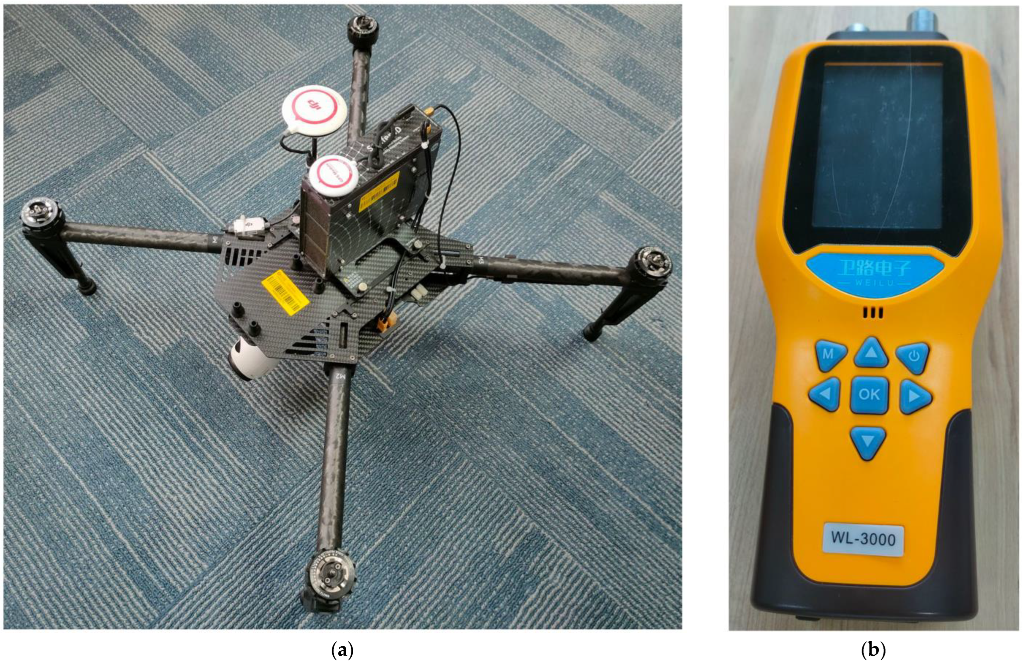
Under the upcoming Energy Efficiency Conservation Act by the Malaysian government, thermal energy will also be regulated and must be reported [10]. However, self-reported energy and emissions data, particularly thermal data lacking a specific meter such as a power meter that can be monitored in real time and verified by an electricity utility provider, may be difficult to verify. Thus, remotely sensed (RS) data from either satellite and or lower altitude platforms such as UAV, may aid in providing report on concentration of GHGs on-site and their changes over time, which can invariably be used to infer emissions sources and rate. We embarked on a full RS study on deriving the changes in concentration of GHGs in industrial areas, focusing on both the use of: (i) UAV-sensor for large-scale near-surface mapping; and (ii) satellite image-based for larger area extent concentration mapping. This article focuses on UAV-based GHGs concentration mapping from industrial areas, and part two of the study to be published next will report the large area satellite-based GHGs concentration mapping.

Previously, studies were conducted on mapping GHG emission using UAV [11,12], pollution concentrations [13,14], GHG emissions using satellite observations [15,16], prediction of carbon dioxide (CO₂) concentration and emission inventories [17,18,19], and biogas potential from plants and manure [20,21]. However, most of these previous studies were mainly on GHG extracted from transportation and vegetation. Indeed, it would be a crucial and desirable goal if the concentration and changes of CO₂, CH₄, and other GHGs in the industrial areas could be systematically mapped. To achieve this, precise mapping and continuous measurement of CO₂ and CH₄ concentrations over a large area and at a periodical/temporal scale with disruptive technology, such as the use of sensors on the drone, calibrated with minimal ground source measurement, is necessary. In addition, the corresponding O₃, NO₂, and SO₂ concentrations could also be determined to complement the CO₂ and CH₄ concentration mapping.

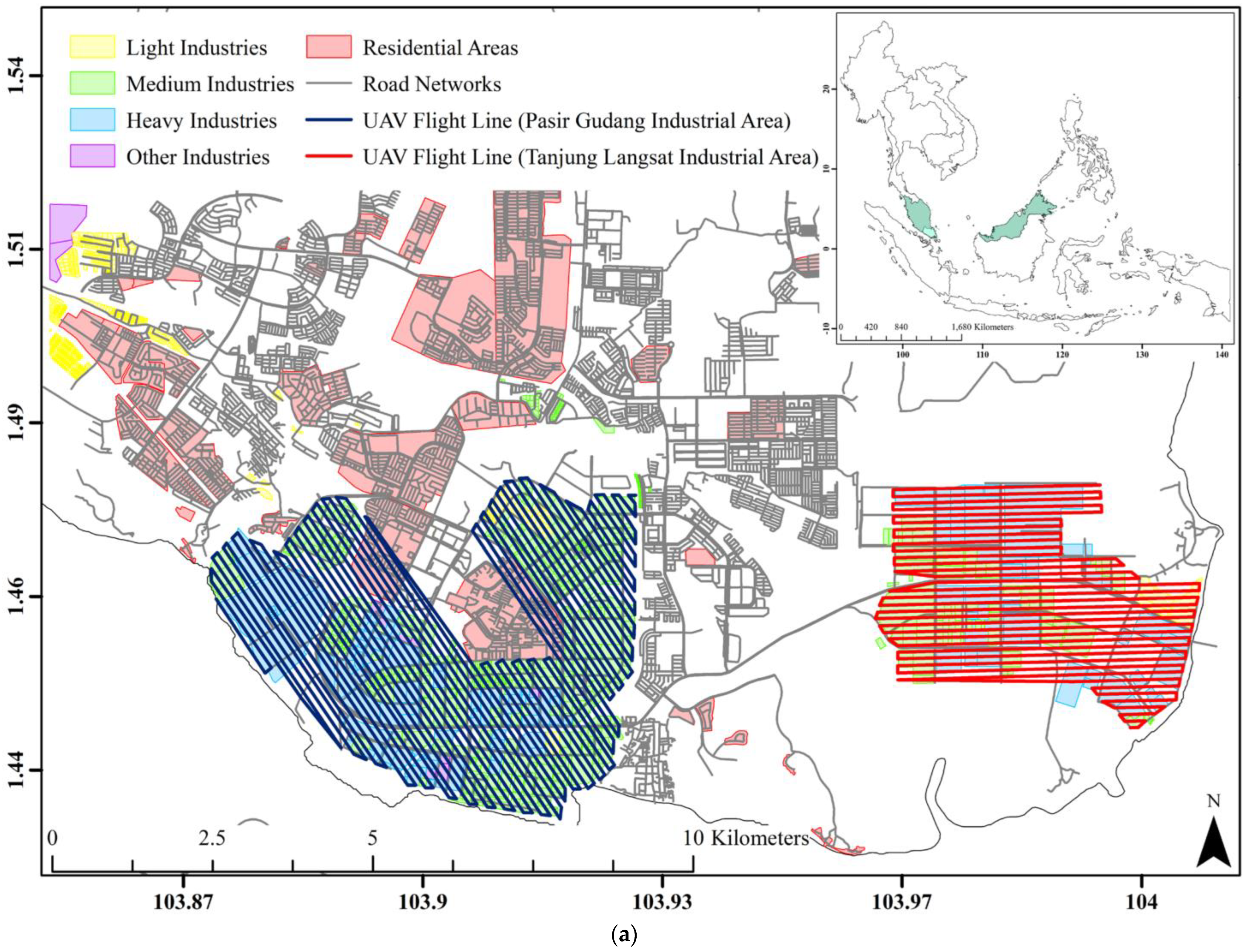
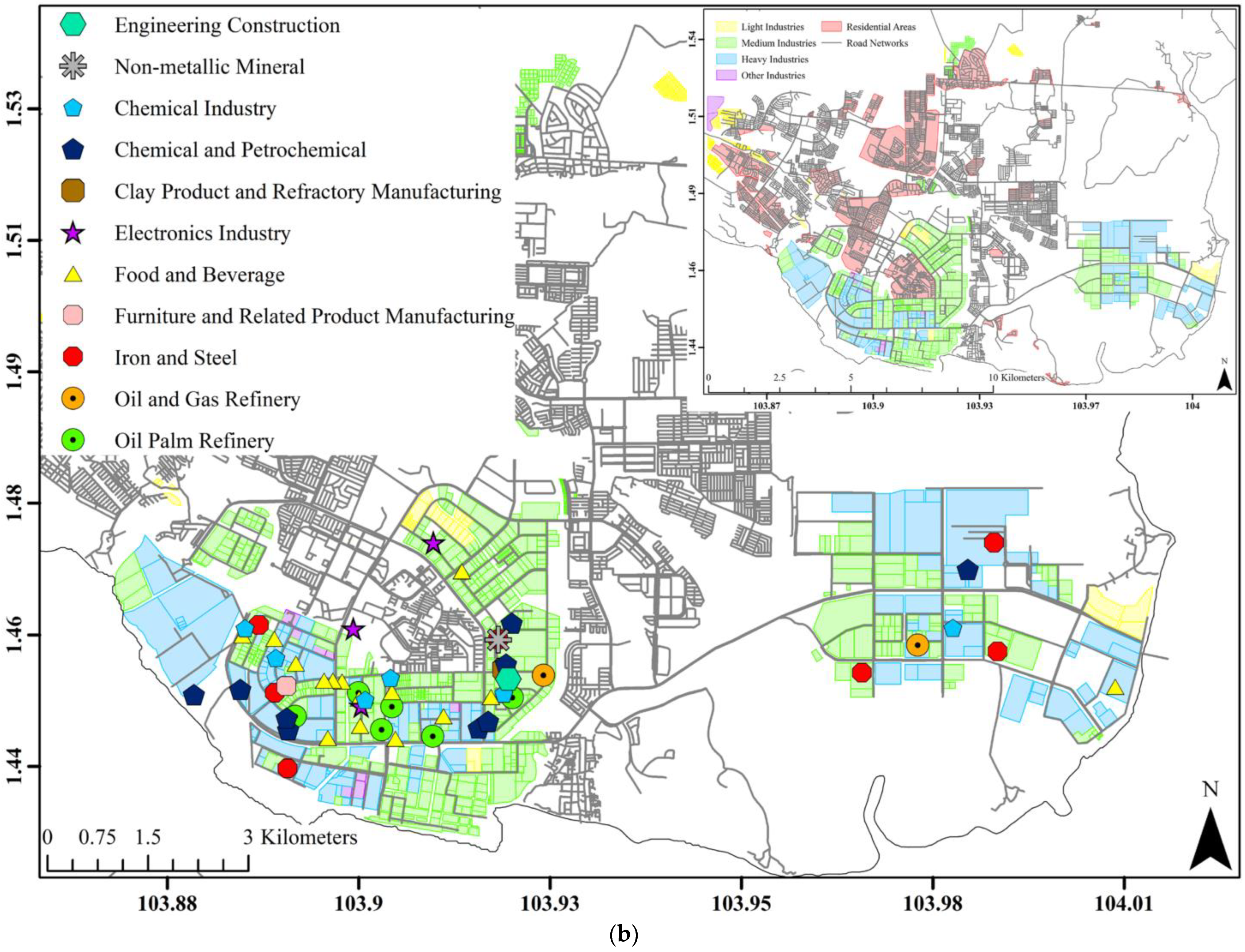
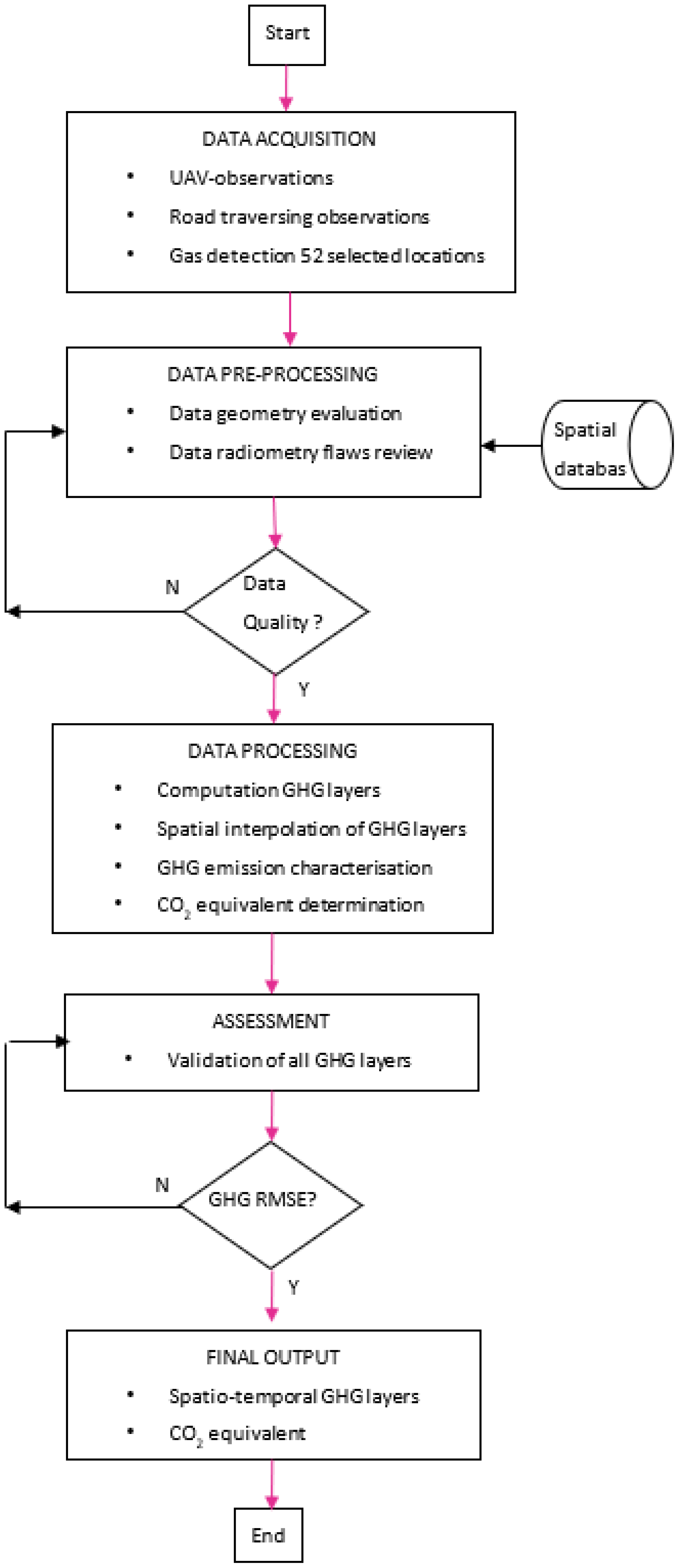
This study, therefore, used a UAV sniffer-based sensor to map changes in GHGs concentration from industrial areas, which is a multi-step approach that can effectively map changes in GHG over an area; this established mapping procedure could be repeated to areas of various sizes permissible pending the range of the UAV-navigation radius. The specific objectives are (a) to characterize the spatial and temporal pattern of the concentration of GHGs (CO₂, CH₄, O₃, NO₂, and SO₂) with emphasis on industrial areas and adjacent residential areas; and (b) to examine and analyse the GHG concentration range based on industry sectors, namely chemical and petrochemical, chemical industry, clay products and refractory, electronics industry, engineering construction, food and beverages, furniture and related products, iron and steel, oil and gas refinery, and oil palm refinery. This spatiotemporal mapping of the concentration of CO₂, CH₄, and other GHGs could later serve for inferring GHGs emissions, assisting in low-carbon planning and speeding up the accomplishment of the 2030 agenda on issues related to sustainable development goal 13, which encourage taking urgent action to combat climate change and its impacts.

2. Materials and Methods

2.1. Study Area

The study areas are the Pasir Gudang and Tanjung Landsat industrial areas. The two industrial areas were employed in the setup for continuous CO₂ and other GHG concentration mapping and monitoring. The Pasir Gudang industrial area (PGIA) is one of the homes of heavy industries in southern Peninsular Malaysia. The PGIA is situated along the Johor State south-eastern tip, covering an area of 1568.673 ha. The area grew rapidly due to the petrochemical and palm oil industries. It is now home to about 300 local and multinational companies, which comprise large-, medium-, and light-scale industries. The main industries at the PGIA include electronics and electrical, research and development, chemicals, food products, engineering-based, and plastics industries. The area is known as the location of the foremost Johor Port as well as the most vital industrial township within the Peninsular Malaysian southern region. The Tanjung Landsat industrial area (TLIA) is located beside the PGIA and covers a total area of about 812.210 ha. TLIA is a fully equipped integrated industrial park and is among the very few industrial parks within southern Malaysia specially chosen for heavy industrial sites. The industry sectors involve chemicals, construction, palm oil, tank storage, warehousing, marine supply, and port services. TLIA is also located close to major seaports, an international airport, and Singapore. The two industrial locations offer jobs to more than 70,000 people. Figure 1 demonstrates the extent of the study areas.

2.2. Materials

The study utilises two important material sets, namely images derived from (a) a UAV-based sniffer4D sensor and (b) a portable GHG detector. The sniffer4D sensor is attached to the UAV for measuring GHGs concentration over relatively large industrial areas in Pasir Gudang (PG) and Tanjung Langsat (TL), while the portable GHG detector is used to measure GHG at ground level at selected locations near real-time of the UAV flight, utilised in calibrating the UAV measurement. Figure 2 depicts the UAV-based sniffer4D sensor and portable gas detector, respectively. The technical details of the sniffer sensor and UAV platform used in this study are shown in

Table 1. Technical specification for UAV-based CO₂ and other GHG emission detection: (a) Sniffer sensor; and (b) the platform.

(a) UAV and portable ground sensor. (Source; Soarability, (2020))
Sensor/Brand/Model	Size	Weight	Resolution/Response Time	Gas Detector
Sniffer4D	150 × 148 × 50 mm	600 g	1 ppm/1 s	CO2, CH4, CO, O3 + NO2, and SO2
Portable gas meter/Weilu/WL-3000	157 × 84.5 × 59.5 mm	365 g	0.1 ppm/3 s	CO2, SO2, NO2, CH4
(b) UAV platform (Source; DJI, 2020.)
Brand/Model	Drone Type	Weight	Brand/Model	Drone Type
DJI Matrice 100	Quadra copter	DJI Matrice 100	Quadra copter	DJI Matrice 100

.

The Sniffer4D Sensor (Table 1a) is a detection and mapping system for GHG concentration data collection. The sensor can be mounted on various platforms, including UAVs, and also works at ground level. The sensor is equipped with a mapping system, able to capture, visualise, and analyse georeferenced and time-stamped gas concentrations. Up to five GHGs can be sensed simultaneously, and the data can be viewed in real time. The five GHGs sensed are methane (CH₄), carbon monoxide (CO), carbon dioxide (CO₂), mixture of ozone and nitrogen dioxide (O₃ + NO₂), and sulfur dioxide (SO₂).

The UAV is a quadcopter flying platform (Table 1b) that has an expandable centre-frame that allows it to mount the sniffer sensor. An extra battery compartment was installed to carry the second intelligent flight battery for an extended flight time of up to 40 min. With the built-in API control feature, navigation for flight missions have been managed comprehensively from planning to execution.

2.3. Methods

2.3.1. UAV Data Acquisition

To obtain the CO₂, CH₄, and other three GHG elements (CO, O₃ + NO₂, and SO₂), the UAV-based data collection approach was used. These five gases were acquired in the study area from a field campaign between 15 and 21 October 2020. The data collections were performed using the Sniffer4D sensor, where the flight plans of the study area were designed prior to the data acquisition. The UAV was flown at an altitude of 100 m for data collection. The flight lines and size of the area for the data collection are shown in Figure 1, while the detailed executed data acquisition mission is tabulated in

Table 2. UAV data acquisition missions.

	PGIA *	TLIA *
Date of data acquisition	15–21 October 2020	15–21 October 2020
Time of data acquisition	0000; 0600; 1200; 1800	0000; 0600; 1200; 1800
Average temperature Min/Max (°C)	24/33	24/33
Average wind speed (km/h)	3	3
Wind direction (bearing)	350°	350°
Period of data acquisition (mins)	245	148
Area of data acquisition (ha)	1837	1177
Total image/files	2880	1090
Front overlap (%)	30	30
Side overlap (%)	30	30
Flight speed (m/s)	15	15
Flight altitude (m)	100	100
Flight direction (bearing)	56°	182°

* Notes: PGIC—Pasir Gudang Industrial Area; TLIA—Tanjung Langsat Industrial Area.

. The GHGs in all areas in Figure 1 were collected in near real-time and 1 h before and after UAV data acquisition using the Sniffer4D sensor and portable gas detector installed on a car-platform traversing the planned road network to cover the entire study area.

2.3.2. In Situ Data Acquisition

Corresponding in situ surface GHG concentration observations were performed continuously during the period of UAV data acquisition and also one hour before and after UAV flight. A portable GHG detector was used to record the GHGs concentration at selected 52 points to represent the 11 industrial sectors: chemical and petrochemical; chemical industry; clay products and refractory; electronics industry; engineering construction; food and beverages; furniture and related products; iron and steel; oil and gas refinery; oil palm refinery; and non-metallic mineral.

In addition, the corresponding surface temperatures at all these 52 points were also observed using field thermal infrared camera. These temperatures were used as additional information on the surface temperature of the industrial targets where GHG concentrations were observed.

2.3.3. Data Processing of UAV Data

The data processing involved two main tasks: data preprocessing and feature extraction for the mapping of GHG concentration. Figure 3 illustrates the flowchart of the entire stages of the data processing. The data processing tasks were performed using Sniffer4D Mapper software, Arc GIS v10.1, Quantum GIS (QGIS) and Digital Image Processing System (ENVI v5.0).

In the data preprocessing stage, two main tasks are performed: firstly, ensuring all the UAV acquired data were geometrically corrected to the local mapping system of the area; and secondly, the radiometric data calibration to reduce the GHG concentration at the flying altitude to a level corresponding to near-surface GHG concentration. The calibration was carried out independently by employing linear regression of UAV-Sniffer observations against the corresponding in situ GHG observations. The calibration functions yielded are shown in Figure 4. Applying these calibration functions to the UAV-GHG observation yields adjusted absolute GHG concentration.

Table 3. Calibrated GHG concentration data.

GHG	Mean * (mg m−3/µg m−3)	Std.dev
CO2	633.038	28.045
CH4	303.054	10.667
CO	1.872	0.909
O3 + NO2	156.162	18.069
SO2	23.163	2.176

* Notes: the unit for CO₂, CH₄, and CO is in mg m⁻³, and unit for O₃ + NO₂ and SO₂ is in μg m⁻³.

tabulates the summary of the GHG concentration derived from the calibrated concentration data with respect to the area of study.

The data processing involves the mapping of the five GHG concentrations into separate layers, each representing CO₂ and the other four greenhouse gases—CH₄, CO, O₃ + NO₂ mixture, and SO₂. UAV data processing for mapping GHG concentration is elaborated in the following sections.

2.3.4. Mapping of CO₂ and Greenhouse Gasses

The mapping of CO₂ and other GHG concentrations starts with the densification of the gas spatial distributions and observations of the daily concentration throughout the mission period over the area of study. This is accomplished using an interpolation process where the concentration of gases at unknown points at selected regular planimetric locations were determined. The Inverse Distance Weighted (IDW) interpolation technique of the QGIS software was used on the data with the same layer extent. The interpolation parameters set for the IDW are (i) the distance coefficient (P: 2) and (ii) the output raster pixel size (X and Y: 10 m). The main input is the mean daily GHG concentration, i.e., a total of seven layers for a week of field campaign data acquisition period. The output of this interpolation is the average daily GHG concentration.

The outputs created from interpolation were clipped with shapefiles in ArcGIS software for mapping GHG concentration for residential areas and industrial zones (light, medium, and heavy industries) and GHG concentrations against the identified industrial sectors: (1) chemical and petrochemical; (2) chemical industry; (3) clay products and refractory; (4) electronics industry; (5) engineering construction; (6) food and beverages; (7) furniture and related products; (8) iron and steel; (9) oil and gas refinery; (10) oil palm refinery; and (11) non-metallic mineral.

Statistical analyses of GHG concentration were performed to characterize the pattern of GHG concentration in the industrial areas (PGIA and TLIA) and adjacent residential areas. The GHG concentration was characterized based on industrial manufacturing sectors. In this analysis, the GHG concentrations were obtained at 52 validation points, which were also earlier used as inputs in the assessment of the derived GHG concentration with the corresponding in situ observation. In the assessment of GHG concentration, a comparison of both UAV-derived concentration and the corresponding in situ observations was performed at 30 random points from the pool of the 52 known validation points, reporting the root mean square error (RMSE). The analysis of variance (ANOVA), which is a statistical test used for determining the significant difference between categorical groups of data by testing differences of means using variance, was used to report the trend of total GHG concentration with respect to all the industrial sectors. Correlation analysis among these GHG concentrations was also examined to consolidate the ANOVA test. In addition, the surface temperature at the 52 validation points was also observed and analysed in the ANOVA and the correlation analysis to assist in inferring the outcomes of the GHG concentrations, as the rank of hotness among the industrial sectors.

3. Results

3.1. GHG Concentrations and Distribution for the Entire Study Area

The average spatial distribution of all the GHG emission concentrations in the study area is shown in Figure 5, with the magnitude ranges within the industrial zones presented in

Table 4. Average GHG concentration trend in industrial areas (PG and TL) and residential areas.

	Entire Industrial Area		Light Industries		Medium Industries		Heavy Industries		Residential Area
GHG	Mean * (mg m−3/µg m−3)	Std.dev	Mean * (mg m−3/µg m−3)	Std.dev	Mean * (mg m−3/µg m−3)	Std.dev	Mean * (mg m−3/µg m−3)	Std.dev	Mean * (mg m−3/µg m−3)	Std.dev
CO2	625.24	30.67	633.04	28.05	628.04	31.16	614.63	32.82	649.82	14.58
CH4	294.24	8.96	303.05	10.67	289.27	8.05	290.40	8.17	293.72	9.06
CO	1.43	0.59	1.87	0.91	1.29	0.40	1.14	0.46	1.87	0.52
O3 + NO2	149.30	15.63	156.16	18.07	148.44	12.55	143.29	16.26	157.92	9.05
SO2	22.24	1.62	23.16	2.18	22.07	1.22	21.49	1.46	23.42	1.09

* Notes: the unit for CO₂, CH₄ and CO is in mg m⁻³, and unit for O₃ + NO₂ and SO₂ is in μg m⁻³.

. The trend of the spatial concentration of the CO₂ is heavily located in the western-half of the study area, with PGIA as the focal source where the concentrations are dominated, ranging from mid-to-high concentration, while the eastern-half focusing on TLIA has low-to-mid concentration. The other four GHG concentrations follow the same spatial pattern but with different magnitudes of occurrence. CO₂ concentration is the highest among GHG concentration within industrial area zones, with little variation in intensity and respective means of 633, 628, and 614 g/m³ for light, medium, and heavy industrial zones. CO₂ concentration at the residential area recorded a higher mean of 649 mg/m³ compared to 625.235 mg/m³ for the entire industrial area, with a similar trend in the other four GHG concentration. CH₄ is the second most prominent GHG in PGIA and TLIA, with a mean of 303, 289, and 290 mg/m³ for light, medium, and heavy industrial zones, respectively. CH₄ mean concentration in the residential area is at 293 mg/m³.

Table 5. Assessment of GHG concentration maps generated.

GHG Emissions	RMSE *
CO2	7.418
CH4	6.134
CO	0.234
O3 + NO2	8.964
SO2	0.819

* Note: the unit for CO₂, CH₄, and CO is in mg m⁻³, and unit for O₃ + NO₂ and SO₂ is in μg m⁻³.

presents the RMSE of in situ GHG concentrations by gas detector at 30 independent sample points chosen randomly from 52 in situ validation points collected from all industrial sectors in PGIA and TLIA industrial areas relative to the UAV concentration maps. O₃ + NO₂ has the highest RMSE of 8.964, followed by CO₂ and CH₄ with an RMSE of 7.418 and 6.134, respectively. CO has the lowest RMSE of 0.234.

3.2. Characterization of GHG Pattern in the Industrial Sector

Figure 6 depicts the percentage concentration of total GHG in relation to all gases for the industry sectors. Across all the sectors, CO₂ and CH₄ are the main gases as well. However, the concentration of the two main gases varies with the industrial sector with the highest concentration of CO₂ found in the electronics industry and the lowest in engineering construction. While the highest concentration of CH₄ is found in engineering construction and the lowest is found in food and beverages. The temperature of the respective industries’ activities was also added in the analysis and shown as a good indicator for GHG concentrations.

The ANOVA test was further conducted to confirm GHG concentration variations with respect to industrial activities.

Table 6. ANOVA test for gases by industrial activities (n = 52).

	Mean Square	F-Value	Pr(>F)
SO2	34.77	6.455	0.0142 *
CO2	35.56	6.621	0.0131 *
CO	31.66	5.812	0.0196 *
O3 + NO2	13.16	2.262	0.1390
CH4	5.48	0.917	0.3430
Temperature °C	49.93	9.824	0.0029 **

* Significant result at p < 0.01; ** Significant result at p < 0.001.

summarises the ANOVA test results. The mean square, F-value, and Pr(>F) for the GHG gases concentration are presented. The mean square suggests the average amount of gas concentration from each industry, while the F-value suggests the amount of average difference by industry. Pr(>F) suggests the significant error. Consequently, the result reveals only three GHG concentration, namely SO₂, CO₂, and CO, differ significantly by industrial activity.

In addition, the temperature of these industrial activities also significantly differs among the industrial activities. The other two GHG concentrations, namely O₃ + NO₂ and CH₄, however, are not significantly different among industrial activities. Further investigation into the relationship between GHG concentration and temperature within industrial activities was also carried out, and the results of this correlation analysis revealed that CO₂ is mostly related to all gas types and temperatures (see

Table 7. Correlation analysis of GHG concentration and temperature with the industrial sector (n = 52).

	Temp	SO2	O3NO2	CO2	CO	CH4
Temp	1.00	0.25 **	−0.15	0.46 **	0.01	−0.89
SO2	0.25 **	1.00	0.41 **	0.69 **	0.78 **	−0.25
O3 + NO2	−0.15	0.41 **	1.00	0.48 **	0.73 **	0.16
CO2	0.46 **	0.69 **	0.48 **	1.00	0.60 **	−0.46 **
CO	0.01	0.78 **	0.73 **	0.60 **	1.00	0.00
CH4	−0.89 **	−0.25	0.16	−0.46 **	0.00	1.00

** Correlation significant at p < 0.001.

).

3.3. Changes in GHG Concentration for PGIA and TLIA

Figure 7 depicts the average hourly GHG concentration for the seven-day period of data collection. While

Table 8. Mean concentration of GHGs for entire industrial and residential area through the study period after calibration.

GHG	CH4 (mg m−3)		CO (mg m−3)		CO2 (mg m−3)		O3 + NO2 (µg m−3)		SO2 (µg m−3)
Date	IA *	RA *	IA *	RA *	IA *	RA *	IA *	RA *	IA *	RA *
15 October 2020	198.79	204.80	1.50	1.87	604.59	632.32	166.83	178.42	22.54	24.09
16 October 2020	176.36	174.77	1.53	2.02	612.61	639.25	140.13	146.42	23.10	24.02
17 October 2020	212.24	208.00	1.23	1.51	633.77	665.11	167.23	181.48	23.08	23.90
18 October 2020	399.66	413.96	0.93	1.13	544.15	547.40	134.14	139.30	20.58	21.33
19 October 2020	294.24	293.72	1.43	1.87	625.24	649.82	149.30	157.92	22.24	23.42
20 October 2020	333.22	332.07	1.34	2.02	689.50	710.31	142.72	144.14	21.63	23.69
21 October 2020	445.16	428.74	2.06	2.68	666.80	704.52	144.74	157.73	22.51	23.51

* Note: IA—Industrial Area; RA—Residential Area.

presents the daily average concentration for the five respective GHG changes in GHG concentration for the entire industrial and residential area through the seven-day measurement period.

As earlier noted, CH₄ and CO₂ are the main GHGs with significant concentrations, followed by the O₃ + NO₂ mixture, while CO and SO₂ have relatively insignificant concentrations in both the industrial and residential areas. The lowest concentration of CO₂ and CH₄ were recorded on the same day, i.e., the second over both the industrial and residential areas, while the highest concentration for CO₂ and CH₄ were respectively recorded on the sixth and seventh day. However, for the O₃ + NO₂ mixture, the lowest concentrations over both the industrial and residential areas were recorded on the fourth day (the same day that the lowest CO₂ was recorded), while the highest were recorded on the third day.

4. Discussion

The industrial GHG concentration mapping in this article relies on UAV sniffer4D sensor-based data acquired during a field campaign between 15 October and 21 October 2020, at PG and TL industrial areas. Adjacent residential area GHG concentrations were also mapped accordingly to see the pattern and compare with those of industrial area. It is, however, important to note that the campaign period was at the end of the inter-monsoon two, when wind speed is almost nil. Notwithstanding, the average windspeed in the area then was 3 km/h as presented in Table 2, and the wind is moving in the northerly direction as it is the transition period from the southwest to northeast monsoons.

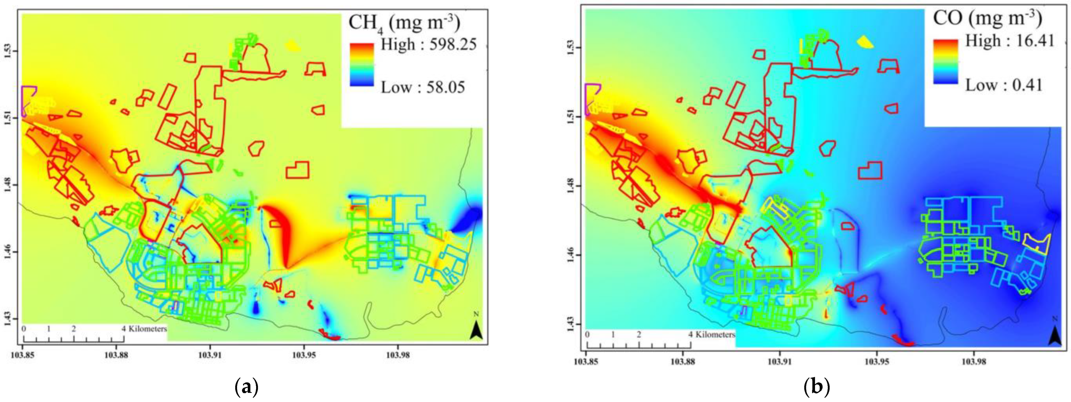
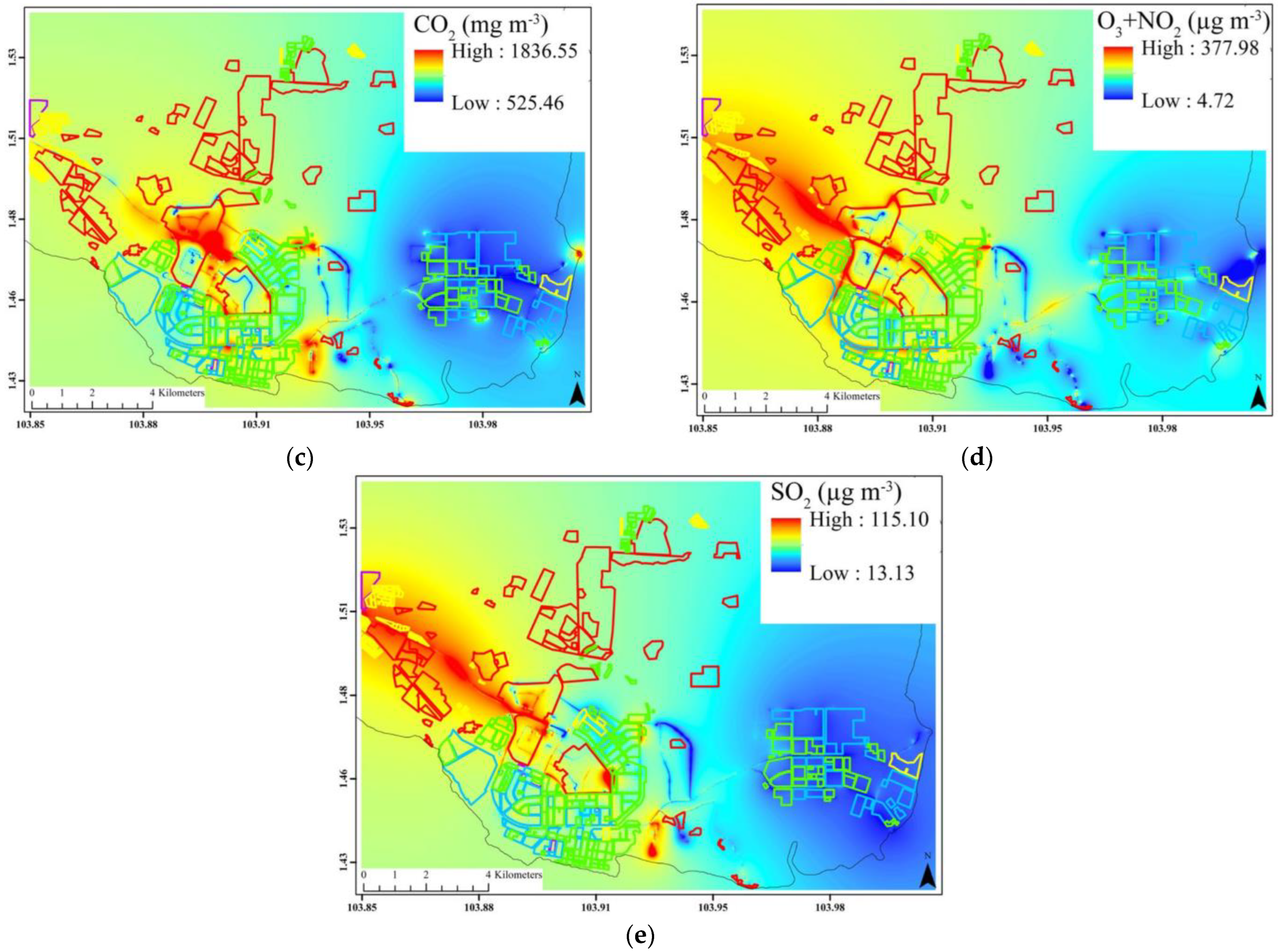
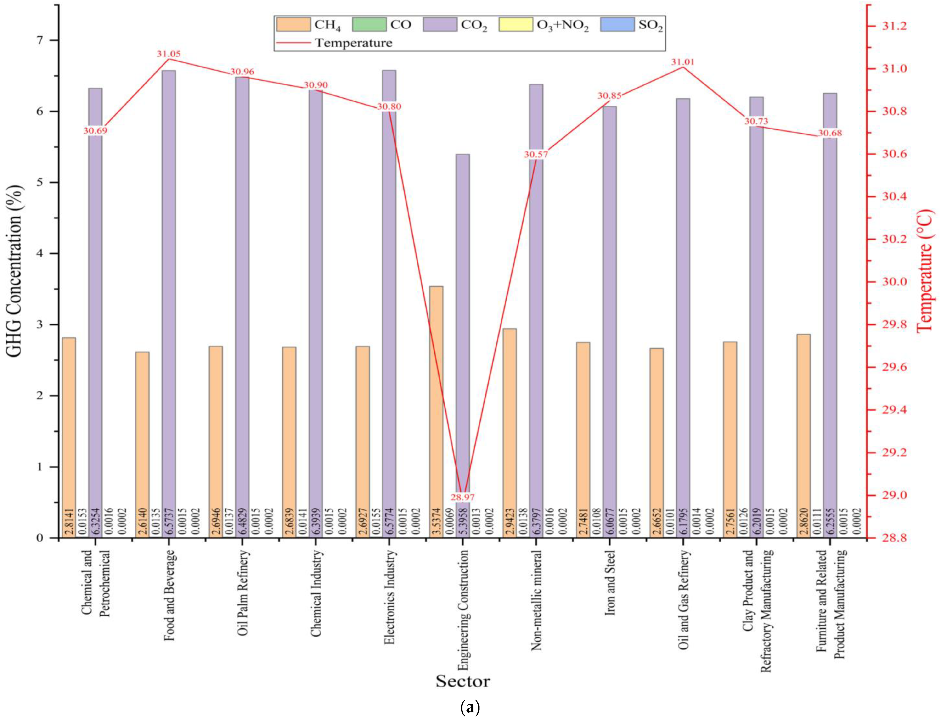
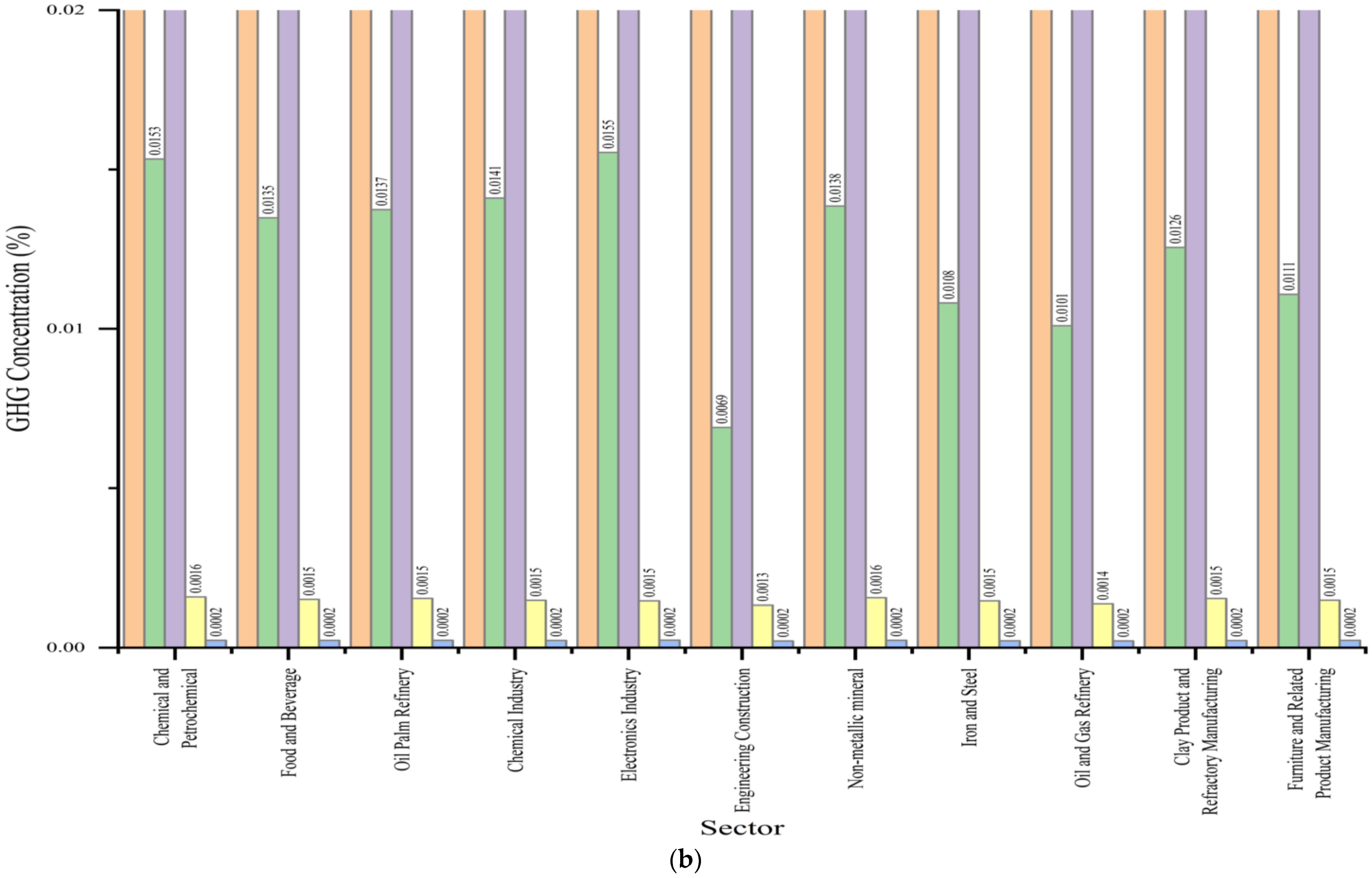
However, this article reveals similar patterns of CO₂, CH₄, CO, O₃ + NO₂, and SO₂ concentration exist between industrial and neighbouring residential areas and among the various industrial zones (light, medium, and heavy) within the industrial areas. Overall, CO₂, followed by CH₄, constitutes the largest GHG concentration among the two industrial areas and within the various zones and sectors. Nevertheless, the GHG concentration does not vary much with industrial activities. The large variability is very prominent in the engineering construction industry, and the least variability is found within oil palm refineries. An intriguing fact is the inversion of the GHG concentration among the three industrial zones, with a slightly higher mean in the lighter industrial zone compared to the medium and heavy industrial zones. However, upon cursory investigations at selected locations, it is noted that most of the factories in the heavy zone, such as refineries, including the oil palm refineries, are equipped with indoor air filtration before releasing it. This, of course, highlights the importance of not overlooking emissions from specific industrial zones or sectors solely based on their kind of activities in low-carbon planning.

Furthermore, this study reveals a higher concentration of GHG over neighbouring residential areas. However, this will not be unrelated to pollution from the industrial areas due to wind transport, as prevailing wind direction during the field campaign shows a northerly flow from the south. 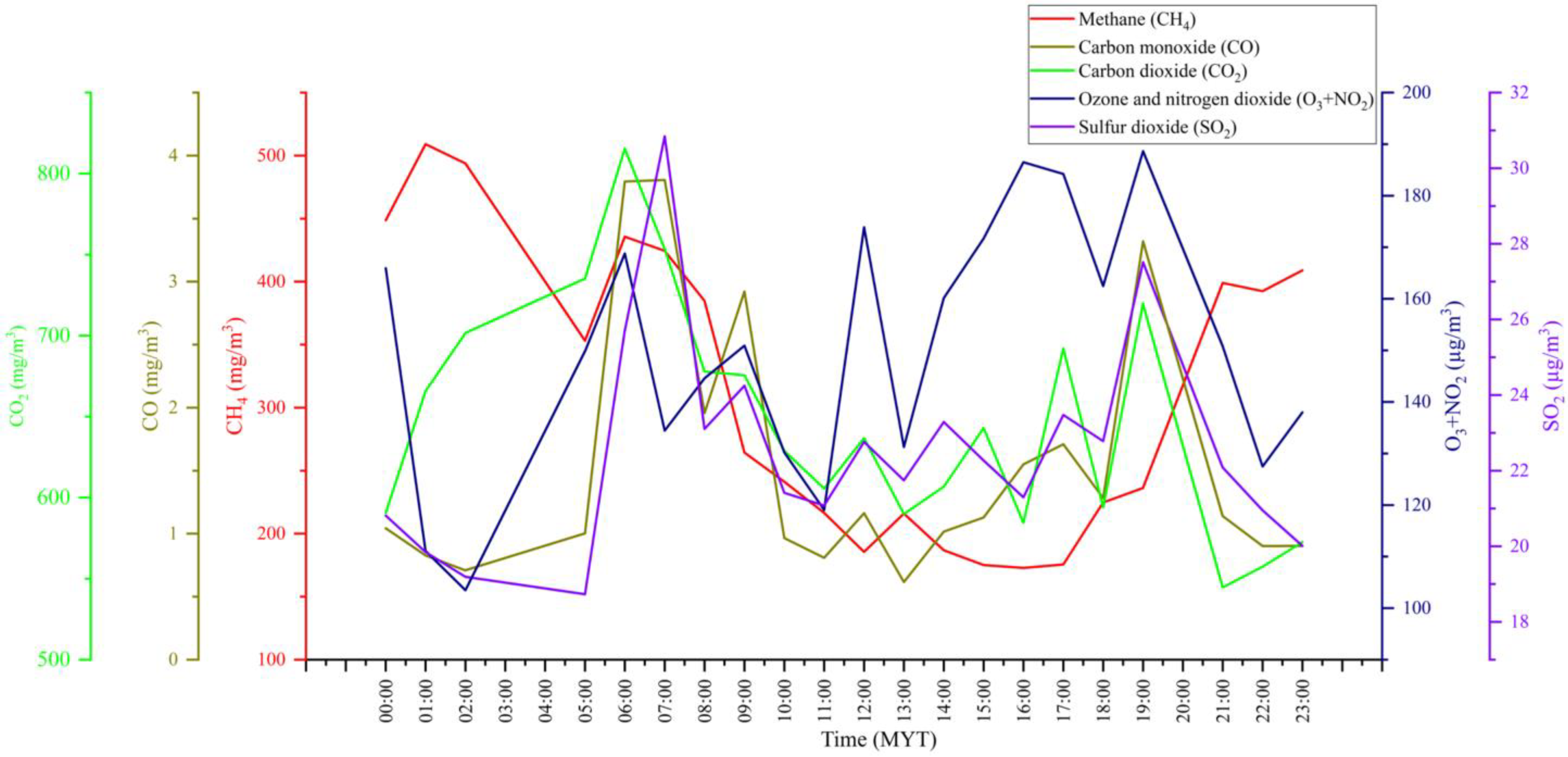Nonetheless, a similar report of higher concentration of GHGs over neighbouring residential areas of industrial areas has long been made about the city of Toronto [22] and 21 countries in Europe between 2007 and 2017 [23]. This calls for a comprehensive look at all environmental components in sectoral land allocations during land-use planning and highlights the need for a cursory look at the concentration of GHGs over residential areas neighbouring industrial areas. Similarly, this study reveals a diurnal temporal variability of GHGs concentrations as seen in Figure 7. This may not be unrelated to the change in the pattern of activities in the respective factories that run 24 h, but characterised by a slowdown of activities during certain times of the day, particularly during labour shift hours. 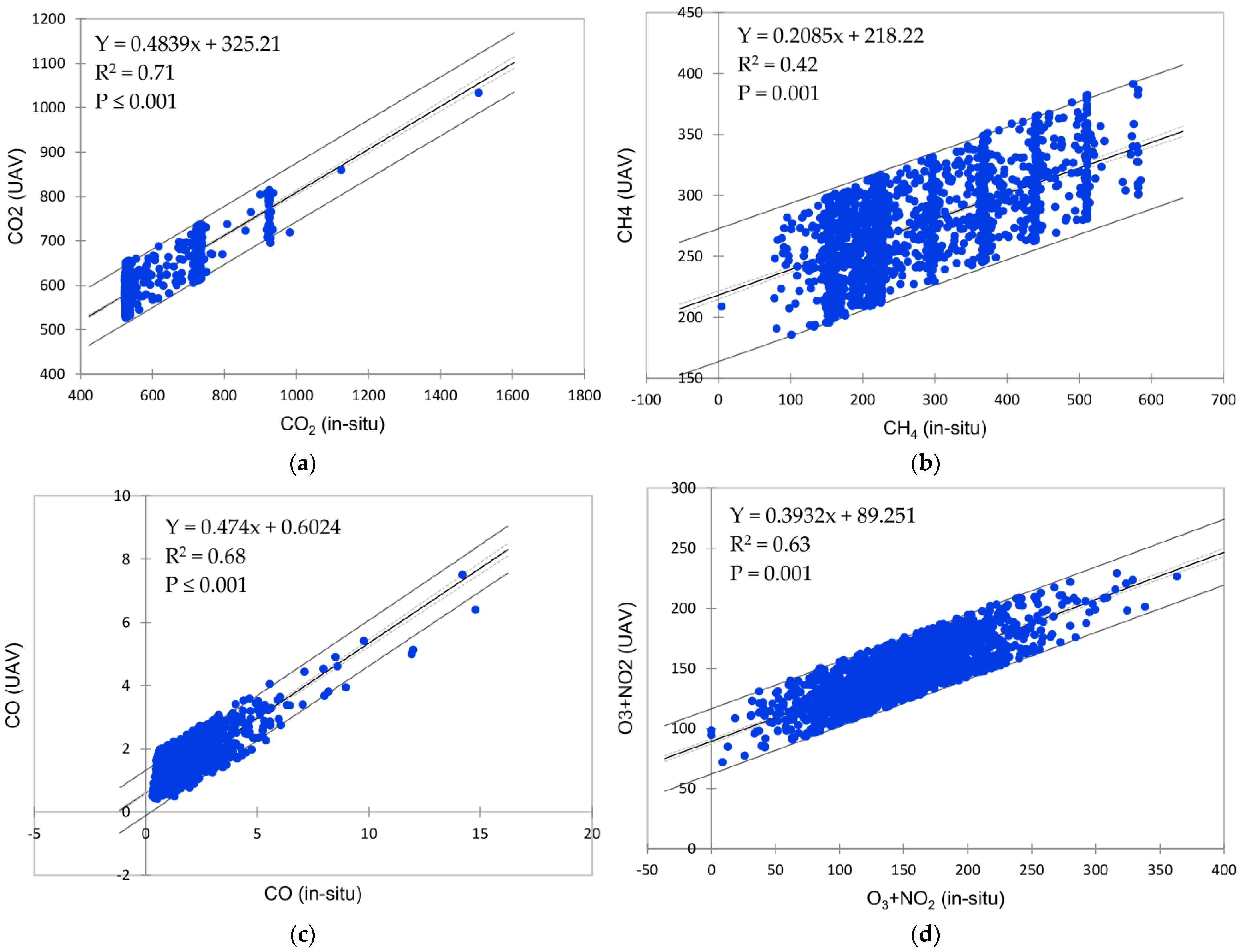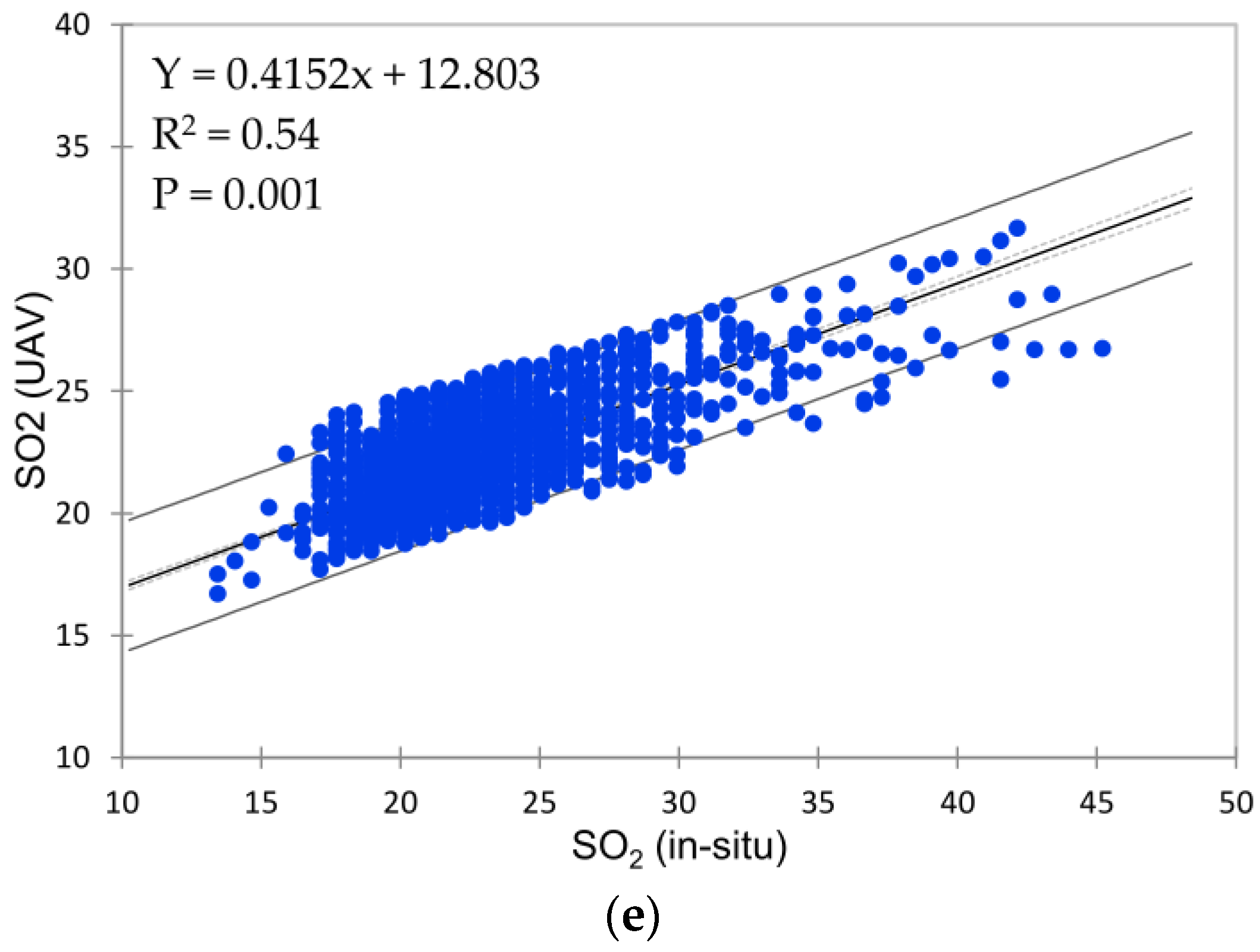Additionally, our one-week campaign also showed a gradual increase in the GHGs concentrations, though with slight variability in some days, particularly on the fourth day of the campaign as presented on Table 8. However, we believe a longer campaign period can reveal a better temporal pattern of GHGs concentration over any industrial area. Finally, the established relationship between GHG concentration and temperature within industrial activities in this study indicates that CO₂ concentration is the best indicator of GHG emissions from fuel burning in industrial areas.

The deployment of UAV for mapping GHG concentration in industrial areas is indeed a step-up initiative towards effective monitoring of GHG emissions and their global warming potential, as well as the realisation of a low-carbon economy (LCE). Aside from the obvious near-ground synoptic measurement, this approach can better detect concentration changes that can be used to infer emission hotspots compared to the use of proxy data. Relative to other approaches for measuring GHG emissions, such as the ground-based level measurements at selected points, the UAV sniffer4D sensor-based approach provides rapid, comprehensive, and yet very cost-effective wider area coverage of GHGs concentration mapping. Thus, this work is very crucial and timely, particularly to Malaysia’s plan to reduce carbon emissions by 45 percent by 2030. With this study’s approach, the baseline and regular status of CO₂ concentration for any specific industrial area with respect to time and date are indeed timely. Similarly, the mapping of GHG concentration in industrial and residential areas may be useful to several private and public sectors concerned about GHG inventory and reduction initiatives, as it could also help individuals or industries gather information that can be used as a reference to prepare a more detailed GHG inventory, which can be used to make inferences about emissions. Nonetheless, industrial areas will continue generating CO₂, CH₄, and NO₂. Once the concentration of these GHGs can be effectively mapped, strategies for their capture can more easily be developed. If this is done, they can be used to make biogas, which will always be a useful source of energy.

5. Conclusions

Industrial manufacturing processes produce a large proportion of GHG emissions due to fossil fuel burning. The Pasir Gudang industrial area, as the focal industrial area, has been a source of pollution that affects the neighbouring areas, including residential areas, resulting in several reported cases of mortality and health-related problems. This study explores the capability of the UAV-based Sniffer4D sensor as a rapid mapping system to characterise the spatial and temporal pattern of the concentration of GHGs (CO₂, CH₄, O₃, NO₂, and SO₂) with emphasis on industrial areas and adjacent residential areas, and examine and analyse the GHG concentration range based on industry sectors, namely chemical and petrochemical, chemical industry, clay products and refractory, electronics industry, engineering construction, food and beverages, furniture and related products, iron and steel, oil and gas refinery, and oil palm refinery. However, this initiative can speed up the accomplishment of the 2030 agenda on issues related to sustainable development goal 13, which encourages taking urgent action to combat climate change and its impacts.

References

1. Manabe, S. Role of greenhouse gas in climate change. Tellus A Dyn. Meteorol. Oceanogr. 2019, 71, 1–13. [Google Scholar] [CrossRef] [Green Version]
2. Smith, A.P. Proof of the Atmospheric Greenhouse Effect. arXiv 2008, arXiv:0802.4324. [Google Scholar]
3. Houghton, J. Global Warming: The Complete Briefing; Cambridge University Press: Cambridge, UK, 2004. [Google Scholar]
4. Halushchak, M.; Bun, R.; Shpak, N.; Valakh, M. Modeling and spatial analysis of greenhouse gas emissions from fuel combustion in the industry sector in Poland. Int. Q. J. 2016, 5, 19–26. [Google Scholar]
5. Clarke, L.; Edmonds, J.; Jacoby, H.; Pitcher, H.; Reilly, J.; Richels, R. CCSP Synthesis and Assessment Product 2.1, Part A: Scenarios of Greenhouse Gas Emissions and Atmospheric Concentrations; US Government Printing Office: Washington, DC, USA, 2006. [Google Scholar]
6. IPCC. Climate change 2013: The physical science basis. In Contribution of Working Group I to the Fifth Assessment Report of the Intergovernmental Panel on Climate Change; Stocker, T.F., Qin, D., Plattner, G.K., Tignor, M., Allen, S.K., Boschung, J., Nauels, A., Xia, Y., Bex, V., Midgley, P.M., Eds.; Cambridge University Press: Cambridge, UK; New York, NY, USA, 2013; Available online: http://www.ipcc.ch/report/ar5/wg2/ (accessed on 5 November 2022).
7. Ministry of Natural Resources and Environment Malaysia. Malaysia: Biennial Update Report to the United Nations Framework Convention on Climate Change. 2015. Available online: https://unfccc.int/sites/default/files/resource/MALBUR1.pdf (accessed on 23 October 2022).
8. Hutchins, M.G.; Colby, J.D.; Marland, G.; Marland, E. A comparison of five high-resolution spatially-explicit, fossil-fuel, carbon dioxide emission inventories for the United States. Mitig. Adapt. Strateg. Glob. Change 2017, 22, 947–972. [Google Scholar] [CrossRef]
9. Malaysia Energy Commission. Efficient Management of Electrical Energy Regulations 2008. Available online: https://www.st.gov.my/images/article/polisi/regulation_suruhanjaya/bi-efficient_management_of__electrical_energy_regulations_2008.pdf (accessed on 20 October 2022).
10. Ashrae Malaysia Chapter. Energy Efficiency and Conservation Act Final Drafting. 2017. Available online: https://www.ashrae.org.my/newsinfo/energy-efficiency-and-conservation-act-final-drafting-1 (accessed on 23 October 2022).
11. Gålfalk, M.; Nilsson Påledal, S.; Bastviken, D. Sensitive Drone Mapping of Methane Emissions without the Need for Supplementary Ground-Based Measurements. ACS Earth Space Chem. 2021, 5, 2668–2676. [Google Scholar] [CrossRef] [PubMed]
12. Mlambo, R.; Woodhouse, I.H.; Gerard, F.; Anderson, K. Structure from Motion (SfM) Photogrammetry with Drone Data: A Low Cost Method for Monitoring Greenhouse Gas Emissions from Forests in Developing Countries. Forests 2017, 8, 68. [Google Scholar] [CrossRef] [Green Version]
13. Afzali, A.; Rashid, M.; Afzali, M.; Younesi, V. Prediction of air pollutants concentrations from multiple sources using AERMOD coupled with WRF prognostic model. J. Clean. Prod. 2017, 166, 1216–1225. [Google Scholar] [CrossRef]
14. Spezzano, P. Mapping the susceptibility of UNESCO World Cultural Heritage sites in Europe to ambient (outdoor) air pollution. Sci. Total Environ. 2021, 754, 142345. [Google Scholar] [CrossRef] [PubMed]
15. Buchwitz, M.; Reuter, M.; Schneising, O.; Hewson, W.; Detmers, R.G.; Boesch, H.; Hasekamp, O.P.; Aben, I.; Bovensmann, H.; Burrows, J.P. Global satellite observations of column-averaged carbon dioxide and methane: The GHG-CCI XCO2 and XCH4 CRDP3 data set. Remote Sens. Environ. 2017, 203, 276–295. [Google Scholar] [CrossRef] [Green Version]
16. Van Beijma, S.; Chatterton, J.; Page, S.; Rawlings, C.; Tiffin, R.; King, H. The challenges of using satellite data sets to assess historical land use change and associated greenhouse gas emissions: A case study of three Indonesian provinces. Carbon Manag. 2018, 9, 399–413. [Google Scholar] [CrossRef] [Green Version]
17. He, Z.; Lei, L.; Zhang, Y.; Sheng, M.; Wu, C.; Li, L.; Zeng, Z.C.; Welp, L.R. Spatio-temporal mapping of multi-satellite observed column atmospheric CO2 using precision-weighted kriging method. Remote Sens. 2020, 12, 576. [Google Scholar] [CrossRef] [Green Version]
18. Wang, K.Y.; Wang, J.L.; Liu, W.T. Ambient carbon dioxide concentrations in industrial park areas: A monitoring and modeling study. Atmos. Pollut. Res. 2014, 5, 179–188. [Google Scholar] [CrossRef]
19. Zeng, Z.C.; Lei, L.; Strong, K.; Jones, D.B.; Guo, L.; Liu, M.; Deng, F.; Deutscher, N.M.; Dubey, M.K.; Griffith, D.W. Global land mapping of satellite-observed CO2 total columns using spatio-temporal geostatistics. Int. J. Digit. Earth 2017, 10, 426–456. [Google Scholar] [CrossRef] [Green Version]
20. Scarlat, N.; Fahl, F.; Dallemand, J.F.; Monforti, F.; Motola, V. A spatial analysis of biogas potential from manure in Europe. Renew. Sustain. Energy Rev. 2018, 94, 915–930. [Google Scholar] [CrossRef]
21. Spyridonidis, A.; Vasiliadou, I.A.; Akratos, C.S.; Stamatelatou, Κ. Performance of a Full-Scale Biogas Plant Operation in Greece and Its Impact on the Circular Economy. Water 2020, 12, 3074. [Google Scholar] [CrossRef]
22. VandeWeghe, J.R.; Kennedy, C. A Spatial Analysis of Residential Greenhouse Gas Emissions in the Toronto Census Metropolitan Area. J. Ind. Ecol. 2007, 11, 133–144. [Google Scholar] [CrossRef]
23. Zhang, Y.; Abbas, M.; Koura, Y.H.; Su, Y.; Iqbal, W. The impact trilemma of energy prices, taxation, and population on industrial and residential greenhouse gas emissions in Europe. Environ. Sci. Pollut. Res. 2021, 28, 6913–6928. [Google Scholar] [CrossRef] [PubMed]
Figure 1. Study area: (a) Pasir Gudang and Tanjong Langsat Industrial Area; and (b) industrial sectors.
Remotesensing 15 00255 g001aRemotesensing 15 00255 g001b
Figure 2. (a) UAV-based sniffer4D sensor; and (b) portable gas detector.
Remotesensing 15 00255 g002
Figure 3. Flowchart of the entire stages of the data processing applied in this study.
Remotesensing 15 00255 g003
Figure 4. Calibration functions of GHG generated using linear regression analysis of UAV observations versus in situ ground measurement: (a) CO2, (b) CH4, (c) CO, (d) O3 + NO2 mixture and (e) SO2.
Remotesensing 15 00255 g004aRemotesensing 15 00255 g004b
Figure 5. Average GHG concentration of entire Pasir Gudang and Tanjung Langsat area: (a) CH4; (b) CO; (c) CO2; (d) O3 + NO2; and (e) SO2.
Remotesensing 15 00255 g005aRemotesensing 15 00255 g005b
Figure 6. Average GHG concentrations and temperature of different industrial sectors (n = 52). Note: the colours of the other GHG bars are too small to be seen in (a), as such they are exaggerated in (b).
Remotesensing 15 00255 g006aRemotesensing 15 00255 g006b
Figure 7. Hourly GHG concentration graph (based on average of 7 days of data). Note: MYT—Malaysia Standard Time.
Remotesensing 15 00255 g007