The Impact of the Type and Spatial Resolution of a Source Image on the Effectiveness of Texture Analysis

Abstract

This paper presents a study on the effectiveness of texture analysis of remote sensing imagery depending on the type and spatial resolution of the source image. The study used the following image types: near-infrared band, red band, first principal component, second principal component and normalized difference vegetation index images of pixel size from 2 m to 30 m, generated from a multispectral WorldView-2 image. The study evaluated the separability of the selected pairs of the following land cover classes: bare soil, low vegetation, coniferous forest, deciduous forest, water reservoirs, built-up areas. The tool used for texture analysis was granulometric analysis based on morphological operations—one of less popular methods which, however, as demonstrated by previous studies, shows high effectiveness in separating classes of different texture. The conducted study enabled researchers to evaluate the significance of image type and resolution for visibility of texture in the image and the possibility of using texture to differentiate between classes. The obtained results showed that there is no single, universal combination of conditions of texture analysis, which would be the best from the point of view of all classes. For most of the analyzed pairs of classes, the best results were obtained for the highest spatial resolution of the image (2–3 m), but the class of built-up areas stands out in this comparison—the best distinction was obtained with the average spatial resolution (10–15 m). Research has also shown that there is no single type of image that is universally the best basis for texture analysis. While for the majority of classes the image of the first principal component was the best, for the class of built-up areas it was the image of the red channel.

1. Introduction

Texture is one of the most important spatial features of an image [1] and including it in the classification process can improve (even significantly) its results. This is shown by numerous examples of the spectral–textural approach to classification, the approach that uses the products of various texture analysis methods [2,3,4,5,6,7,8,9,10,11,12,13,14,15,16,17]. Texture is also an important spatial feature to take into account in the process of object-oriented image classification [5,9,10,11,18,19]. It is also used in the analysis of other types of images, e.g., medical ones [20,21,22]. It should be noted that it is also one of the easiest features to incorporate in image processing, because it does not require prior segmentation of an image. While the size of an object or its shape is closely related to the object, and as such requires the extraction of an object/segment in order to determine its characteristics, texture tends to be defined in relation to the neighborhood of a pixel (e.g., within a specific radius), regardless of the object to which the pixel would be assigned. Thanks to this, and unlike other spatial features, texture can also be incorporated in the pixel-based approach to classification because each pixel is assigned the texture (neighborhood) feature individually.

The Cambridge Dictionary defines “texture” as “the degree to which something is rough or smooth or soft or hard”. Referring to an image, “texture” is typically understood as the type, size and mutual relation of elements constituting a given object or a land cover class. However, there is no unambiguous mathematical definition of texture [23], which has led to the development of a multitude of approaches to texture analysis. The most popular method used in image processing, particularly in remote sensing, appears to be the Grey Level Co-occurrence Matrix and a series of measurements based on it, called GLCM or Haralick statistics [2,3,24]. Other methods, like fractal analysis [4], discrete wavelet transformation [25], Laplace filtration [26,27,28], random Markov fields [29,30] and granulometric analysis [31,32], follow a different approach. It is also worth mentioning Convolutional Neural Networks that can also be employed for analyzing the texture of an image.

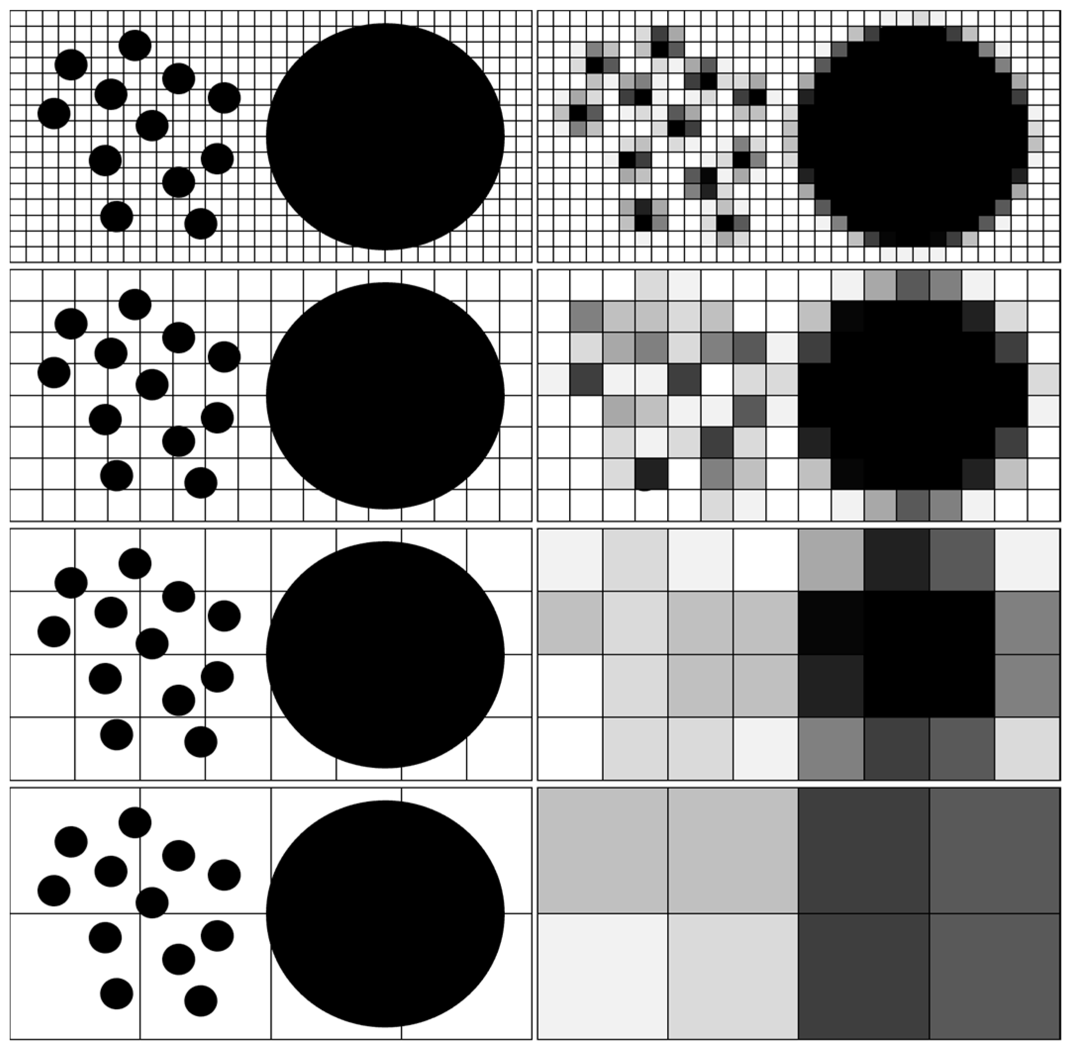
However, regardless of how we analyze “the degree to which something is rough or smooth or soft or hard”, the image of an object’s, or a class of objects’, texture determines to a large extent the effectiveness of the texture analysis. An important factor determining the texture image, in turn, is the spatial resolution of the image itself [33] because it affects whether and how specific elements potentially composing texture will be visible in the image. It is commonly understood, and proving this fact is not the aim of the studies presented below. Instead, it is a systematic analysis of how the type of image affects—both in terms of spatial resolution and spectral type—the perception of texture and its importance in identifying selected classes. The main purpose of this paper is to determine the effect of an image’s spatial resolution on the significance of texture as a feature that enables distinguishing between selected classes of land cover. The effectiveness of different methods of texture analysis for various types of images (most often of high or very high spatial resolution) has been widely studied and reported in the literature, but relatively few studies have been devoted to the relationship between the texture of the image and its resolution for different classes. This very relationship is examined in the study presented below, and while it is quite understandable that texture gains in importance with the increase in spatial resolution [11] (as shown in Figure 1), and this is confirmed by the results of the spatio-spectral classification [34,35], the exact nature of this phenomenon is not well researched.

While examining this relationship, the study also examined the impact of the source image type on the effectiveness of texture analysis. Texture is a spatial feature, so there is no need to analyze it for each spectral band because all spectral bands present the same arrangement of spatial features (depending on the spatial resolution of the image). It should be noted, however, that each image can display such pattern with different intensity: certain features can be more visible in some spectral bands than in others. Therefore, from the point of view of the effectiveness of texture analysis, it is important to properly select the source image. The source image selection was also investigated in the study presented in this paper. Here, it should be noted that the selection does not need to be limited to spectral bands. A very common choice is the first principal component image [36,37,38] and the NDVI (Normalized Difference Vegetation Index) [39] was also examined. There are also publications proposing other solutions regarding the selection or creation of an appropriate source image for texture analysis [34]. Comparable studies (limited only to assessing the effect of the source image type on the accuracy of texture analysis, excluding other features such as the resolution, which is the main topic investigated in the study reported here) are presented in [40].

In the study reported in this paper, granulometric analysis was used as a tool for texture analysis. It is a slightly less popular method of texture analysis, but it is very effective when compared to other methods (e.g., GLCM) [41,42] due to several important advantages, which are described below.

2. Brief Presentation of Texture Analysis Using Morphological Granulometry

Granulometric analysis is one of many methods of texture analysis. It is definitely less popular than such methods as GLCM or wavelet transform. However, as comparative studies show, it has significant advantages to which it owes its greater effectiveness in the case of texture analysis used to identify selected classes of land cover [31,32]. These advantages include resistance to the edge effect and natural multiscality. Before discussing these advantages, basic information on granulometric analysis will be presented.

Granulometric analysis was developed by Haas et al. [31], giving rise to an entire family of image processing methods called Mathematical Morphology. The technique of mathematical morphology originally consisted in carrying out on a binary image a sequence of morphological openings with a gradually increasing size of a structuring element (SE), and then calculating the differences between the individual images: the original one and the result of the first opening, the result of the first opening and the result of the second opening, etc. Subsequent opening operations with increasing SE size remove elements (brighter than the neighborhood) smaller than the SE from the image, while elements which are not smaller are left unchanged. Based on these differential images, the granulometric density function is calculated for the image. The function describes the occurrence of texture grains in the analyzed image. Local granulometric analysis, consisting of an analysis of a specific neighborhood of each pixel, was later proposed by Dougherty et al. [29], while Vincent [43] presented granulometric analysis on grayscale images. An analysis equivalent to the granulometric analysis, which is based on a series of openings, is an analysis based on a series of closings (sometimes called the antigranulometry) [14]. Both versions of granulometry, based on opening and closing, provide the same type of information (and with the same structure), with the significant difference that one of them (based on opening) carries information on the presence of light grains—texture components, while the other (based on closure)—about dark ones. Their meaning for determining the texture of different classes of objects (and above all—for distinguishing them from each other) may vary, depending on the nature of the texture of each class. Most often, however, both versions of the analysis are used at the same time, treating the information derived from them as complementary. For this reason, we decided to use an analysis based on these two functions.

While the result of the global granulometric analysis is a function of granulometric density characteristic of the entire image, the result of the local analysis is a set of functions assigned to individual pixels, such functions being characteristic of their neighborhoods. This type of information is presented as a set of images called granulometric maps.

The local granulometric analysis resembles the morphological profile proposed by Mura et al. [44,45], with the difference that the morphological profile is based on changes only within the analyzed pixel, while the local granulometric analysis examines changes occurring in a specific neighborhood. Thus, while granulometric analysis provides information about the size of texture grains in the entire neighborhood, the morphological profile—about the size of the grain to which a given pixel belongs. This is a significant difference from the point of view of texture analysis.

Other distinguishing features of granulometric analysis are its multi-scality and resistance to the edge effect.

The edge effect, noticeable in other popular methods of texture analysis, results from the fact that high texture is recognized through high spatial frequency. Places near the edges of objects, even low-texture objects, will therefore be identified similarly as places with high texture, due to high spatial frequency of the near edge. This can result in errors of classification based on such textural information [42]. The granulometric analysis is, as mentioned earlier, practically free of this type of effect because it does not analyze the differences between pixels in a particular neighborhood, as in the case of other texture analysis methods, but the number of removed image elements. Opening and closing operations, which are the basis of this method, remove small (compared to the size of the SE) image elements leaving the remaining ones mostly unchanged. Therefore, as long as an object is not smaller than the SE (and thus not treated as an element of the analyzed texture), the edge of the object will remain intact between successive opening or closing operations. As a result, differential images will not show significant changes in these places.

The second important characteristic of this analysis, which can be called its natural multi-scality, results from the very essence of the analysis which is the performance of a sequence of opening or closing operations with the use of the SEs of increasing sizes. The resulting granulometric maps contain information about the presence of texture elements of different sizes assigned to individual maps. This enables an analysis of texture manifested by different sizes of grains without changing the image resolution. It is worth noting that successive steps of the sequence of openings or closings, and the resulting granulometric maps, provide information about the elements of the image smaller than a given SE and at the same time not smaller than the SE used in the previous step. For example, the analysis made on the basis of images resulting from processing operations using an SE of size 1—which, in simple terms, means the radius of a circle circumscribing a given SE, e.g., a square 3 × 3 pixels—provides information about the presence of elements of a size smaller than 3 pixels, while an analysis made in the next step using SE of size 2 (e.g., a 5 × 5 pixel square) provides information about the presence of elements with a size smaller than 5 pixels but not smaller than 3 pixels.

A certain disadvantage of granulometric analysis, especially in comparison to GLCM, is the inability to analyze the type of organization or distribution of texture grains. While the GLCM analysis consists in calculating various statistics related to particular aspects of the texture, the granulometric analysis only allows us to determine the number of grains of different sizes and relative brightness. However, for the studies presented in this article, this ability was considered less important because the purpose of the study was to analyze the ability to detect texture in general, without referring to its various aspects.

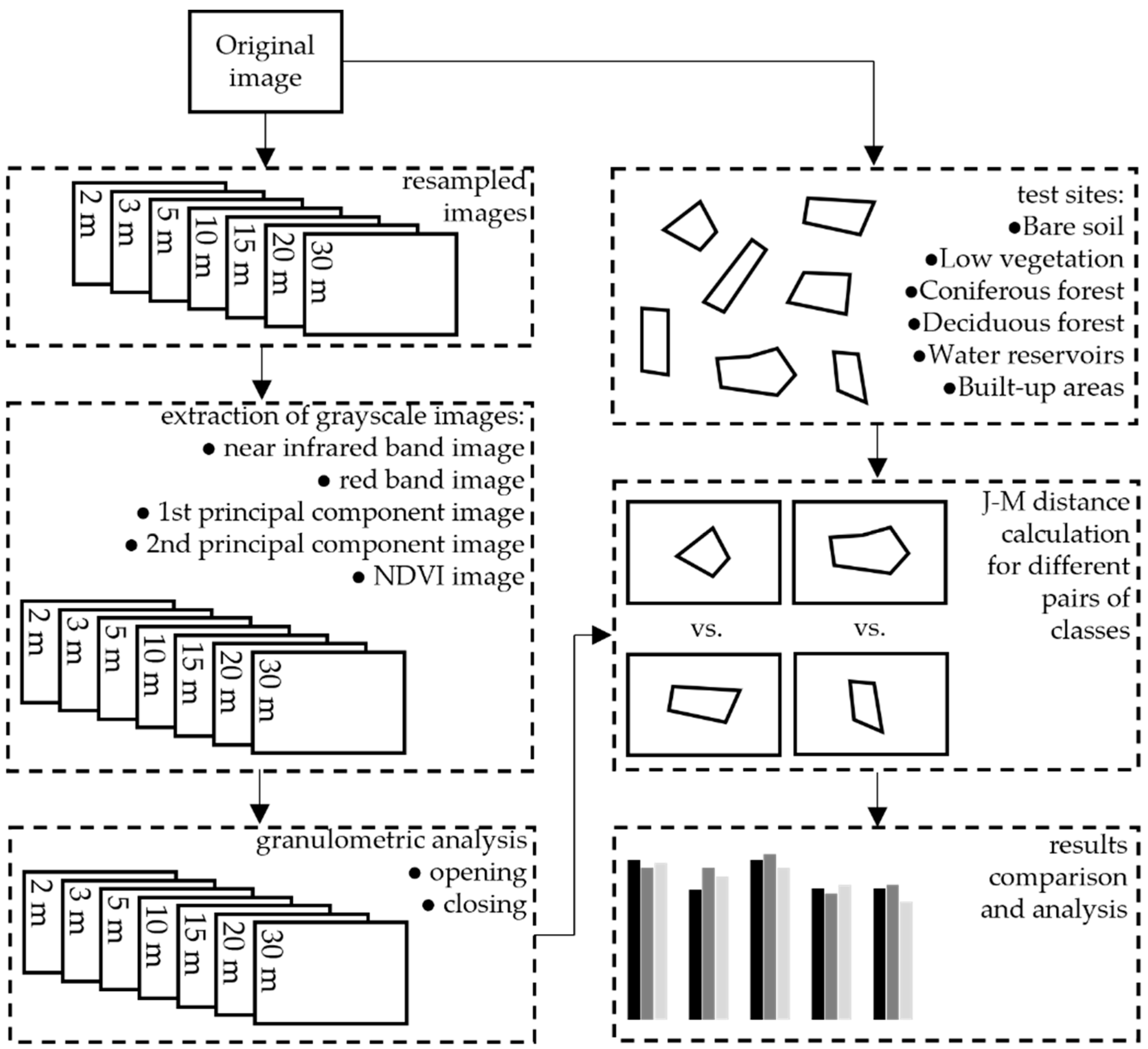
3. Methodology

Two primary objectives of the study were identified. The first objective was to determine the impact of the spatial resolution of an image on the effectiveness of texture analysis for distinguishing some selected (basic) land cover classes. For this purpose, a very high resolution test image was taken and then its resolution was gradually reduced, creating subsequent test images. The second objective of the study was to determine whether, and in what manner, the type of a source image is significant for the effectiveness of texture analysis. Texture, as a spatial feature, is to some extent independent of the spectral features of objects, but it seems justified to put forward a thesis that in some images, e.g., spectral bands or certain products of image processing (spectral indicators, images of principal components, etc.), certain texture features may be more visible than in others. Determining the impact of the source image type on the effectiveness of texture analysis was the second objective of the present study. The scheme of the research methodology is presented in Figure 2.

3.1. Source Image

The study used a multispectral WorldView-2 image, acquired on 4 August 2011, with a pixel size of 1.8 m. All the eight spectral bands collected by the WorldView-2 multispectral scanner were used (Coastal, Blue, Green, Yellow, Red, Red Edge and 2 Near-Infrared bands). The scene covers the area of the southern part of Warsaw in the central–eastern part of Poland. This area is characterized by a diverse land cover and use.

3.2. Selection of Analyzed Pairs of Land Cover Classes

The aim of the analysis was to compare the separability of selected LULC (land use/land cover) classes. For this purpose, 6 land cover classes were selected:

• Bare soil—SOIL
• Low vegetation—VEG
• Coniferous forest—CFR
• Deciduous forest—DFR
• Water reservoirs—WTR
• Built-up areas—BUA

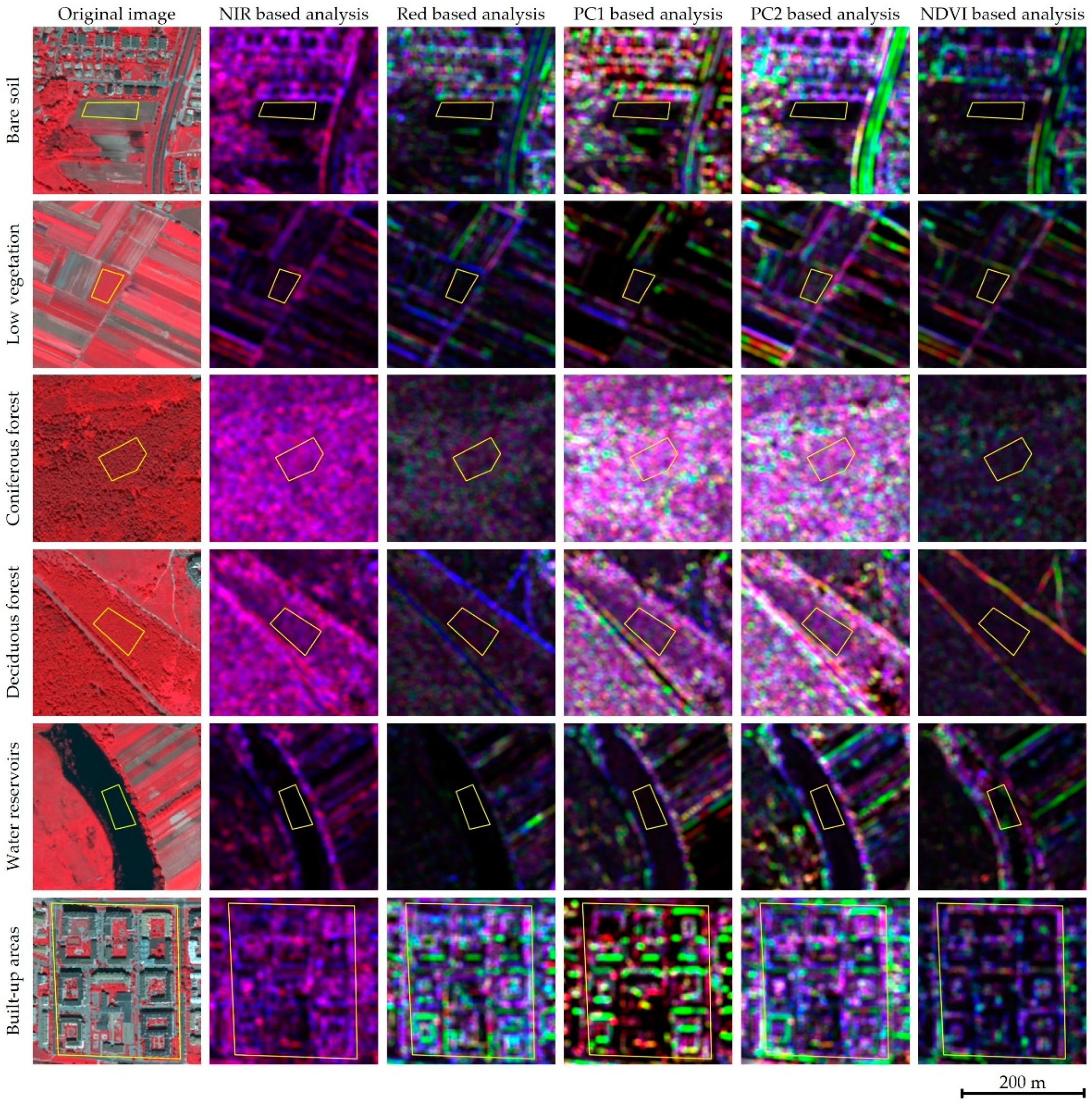
For each of the classes, 5 representative test fields were prepared, of sizes ranging from about a thousand to tens of thousands of pixels.

Selected test fields with exemplary results of texture analysis using granulometric processing are shown further in the text in Figure 3.

Subsequently, the selected classes were combined into pairs to be analyzed. Individual pairs were selected mainly based on their, at least partial, spectral similarity. Pairs of classes which are easily distinguishable by spectral analysis, therefore in their case texture analysis is of secondary (or no) importance, were not analyzed. The following class pairs were selected for further analysis:

• Deciduous forest/low vegetation;
• Coniferous forest/low vegetation;
• Coniferous forest/deciduous forest;
• Low vegetation/built-up area;
• Bare soil/built-up area;
• Coniferous forest/built-up area;
• Deciduous forest/built-up area;
• Water reservoirs/built-up areas.

3.3. Preparation of Images for Analysis

The primary objective of the study was achieved by comparing the values of pixels in selected images (which were the products of texture analysis obtained for individual LULC classes) and then by determining the separability of values for these classes. The preparation of the data was performed in several steps described below.

3.4. Images of Degraded Resolution

Based on the source image, a group of images was generated by degrading the spatial resolution of the main source image. Decreasing the resolution was carried out using the bilinear resampling technique.

These images, together with the main source image, were the basis for further analysis. Individual pixel sizes were selected to correspond to the typical resolutions of satellite images:

• 2 m;
• 3 m;
• 5 m;
• 10 m;
• 15 m;
• 20 m;
• 30 m.

3.5. Generating Types of Images for the Analysis

Next, 5 single-layer (grayscale) images were prepared for each of the multispectral images (including images of decreased resolution). These images were used as source images to examine the impact of the source image type on the effectiveness of texture analysis from the point of view of separating selected classes of land cover (the second of the above-described study objectives). The image types for the analysis are listed below:

• Near-infrared band (NIR) image;
• Red band (Red) image;
• First principal component (PC1) image;
• Second principal component (PC2) image;
• Normalized difference vegetation index (NDVI) image.

In this manner, 35 images (of 7 different pixel sizes and 5 different image types) were created as the basis for the analyses which are described below.

The rationale for the above selection was to present diverse images/products that can be obtained from multispectral data and was based on the experience gained from previous studies [14]. These studies had shown i.a. high effectiveness of texture analysis based on NIR images, the images that present high contrast between the areas covered with vegetation and other areas, with very dark shadows which are the reason for a distinct texture of the classes characterized by the occurrence of tall elements.

The Red image was selected mainly for comparison with the NIR image in order to determine the significance of the spectral band selection for the effectiveness of texture analysis. It is worth noting here that certain imagery may not contain the near infrared spectral band at all (though this is true mainly for historical imagery), hence the attempt to assess the effectiveness of texture analysis of one of the visible spectral bands.

Another image used in the study was the first principal component (PC1) that is characterized by the largest possible global variance of an image, which may (but does not have to) result in high local variances contributing to the distinct texture of certain LULC classes. The second principal component (PC2) image was selected partly for comparison with the PC1 image. It should be noted that in the second principal component (PC2) image the vegetation cover is often emphasized [46,47,48], which may result in a distinct texture of areas with vegetation. The last of the proposed images—NDVI—is by definition used to assess vegetation, and therefore it produces an image potentially useful for LULC classes in which vegetation plays an important role.

We have not included other spectral bands such as shortwave infrared or red edge channels, which may be important for the analysis of selected land cover classes, especially vegetation. This was due to the potentially lower contrast between the illuminated and shadowed areas (which results from the lower albedo in this range) and the fact that these channels are less frequently available in remote sensing systems (satellite or airborne), and in some systems (such as Sentinel-2) they have lower spatial resolution which makes them less useful for texture analysis.

3.6. Texture Analysis of Images

The last step of preparing the source images for the analysis was processing of the 35 earlier generated images using granulometric analysis. It was performed based on morphological opening and closing operations using the structuring elements (SEs) with sizes from 1 to 3 pixels. The size of the SE means in this case a radius of a pseudocircle (a circle according to the system of the pseudo-Euclidean distance). Hence, an SE of size 1 is a pseudocircle with the diameter of 3 pixels, an SE of size 2 is a pseudocircle with the 5 pixel diameter, and an SE of size 3 is a pseudocircle measuring 7 pixels. Obviously, the actual size of the structuring element (measured in meters) changes depending on the image pixel size.

The sizes of the SEs were selected in such manner that even with the image having the smallest pixel it was possible to analyze the essential elements of the texture of all analyzed classes (size 3 of the structuring element with a pixel of 2 m means approx. 14 m).

Another parameter influencing the result of the texture analysis was the size of the neighborhood of a single pixel in which the texture was analyzed. If the selected radius of the neighborhood is large, then all the surrounding elements of the texture will be taken into account, but the texture of the neighboring objects could be included as well. On the other hand, a smaller neighborhood can make it difficult to take into account important features of the texture. For this reason, several possible lengths of neighborhood radii (measured in pixels) were proposed. The length of a proposed neighborhood radius depended on the spatial resolution of the image: for images with a larger pixel size a smaller radius (in pixels) was proposed. They are presented in

Table 1. Neighborhood sizes depending on the image pixel size.

	Analysis Neighborhood Radius (in Pixels)
Pixel Size	Small Radius	Medium Radius	Large Radius
2 m, 3 m, 5 m, 10 m	5 pixels	7 pixels	10 pixels
15 m, 20 m, 30 m	3 pixels	5 pixels	7 pixels

.

Among the described classes it is possible to indicate pairs of classes which are spectrally similar but have clearly different texture (such as low vegetation and forest or built-up areas and bare soil). In such cases, the effectiveness of texture analysis becomes important, even crucial, for the effective identification of these classes. However, the difference in textural information can also be useful for spectrally different classes, also for those with a theoretically similar texture, whether it is high (forests and built-up areas) or low (bare soil and low vegetation).

Figure 3 presents the selected test fields with exemplary results of texture analysis using granulometric processing.

4. Methodology of the Analysis

The main objective of the proposed methodology was to enable the measurement of the separability of the result values of the texture analysis obtained for individual land cover classes.

For each class, 5 representative test fields were prepared. Then, the values obtained for these areas in different test images were compared and the separability of the values was determined. Jeffries–Matusita Distance was used as the measure for the assessment of separability. This is a metric used in remote sensing usually for measuring the separability of the values of training fields in the classification process and for selecting the optimal bands [49]. The criterion of separability between two classes $w_i$ and $w_j$—$J{M}_{ij}$ can be defined as follows [50,51]:

$$J{M}_{ij}=2\left(1-e^{-d_{ij}}\right)$$

where $d_{ij}$ means the Bhattacharyya distance between two classes $w_j$ and $w_{i }$, which can be defined as follows [49,52]:

$$d_{ij}=\frac{1}{8}{\left(m_j-m_i\right)}^T{\left[\frac{{\mathsf{\Sigma }}_i+{\mathsf{\Sigma }}_j}{2}\right]}^{-1}\left(m_j-m_i\right)+\frac{1}{2}ln\frac{\left|\frac{{\mathsf{\Sigma }}_i+{\mathsf{\Sigma }}_j}{2}\right|}{\sqrt{\left|{\mathsf{\Sigma }}_i\right|\left|{\mathsf{\Sigma }}_j\right|}}$$

where $m_i$ and $m_j$ denote the mean values and ${\mathsf{\Sigma }}_i$ and ${\mathsf{\Sigma }}_j$ denote the covariance matrices of the two analyzed classes: respectively, $w_i$ and $w_j$.

JM distance is limited to the $\langle 0;2\rangle$ range of values, with higher value denoting a better separation of the sets. In classification practice it is assumed that two sets (two classes) are completely separated from each other if J–M distance between the classes is larger than 1.8 [53].

In this manner, pairs of test fields were compared with each other in all possible combinations of pairs of classes. The averaged results obtained for specific pairs of classes in different source images were used to assess the effectiveness of texture analysis as a tool enabling to assign individual pixels values allowing to separate specific classes of land cover.

5. Results and Discussion

The results obtained for different pairs of land cover classes are presented and discussed in the subsections below. The section following the subsections presents the summary of all the results obtained for all the analyzed class pairs.

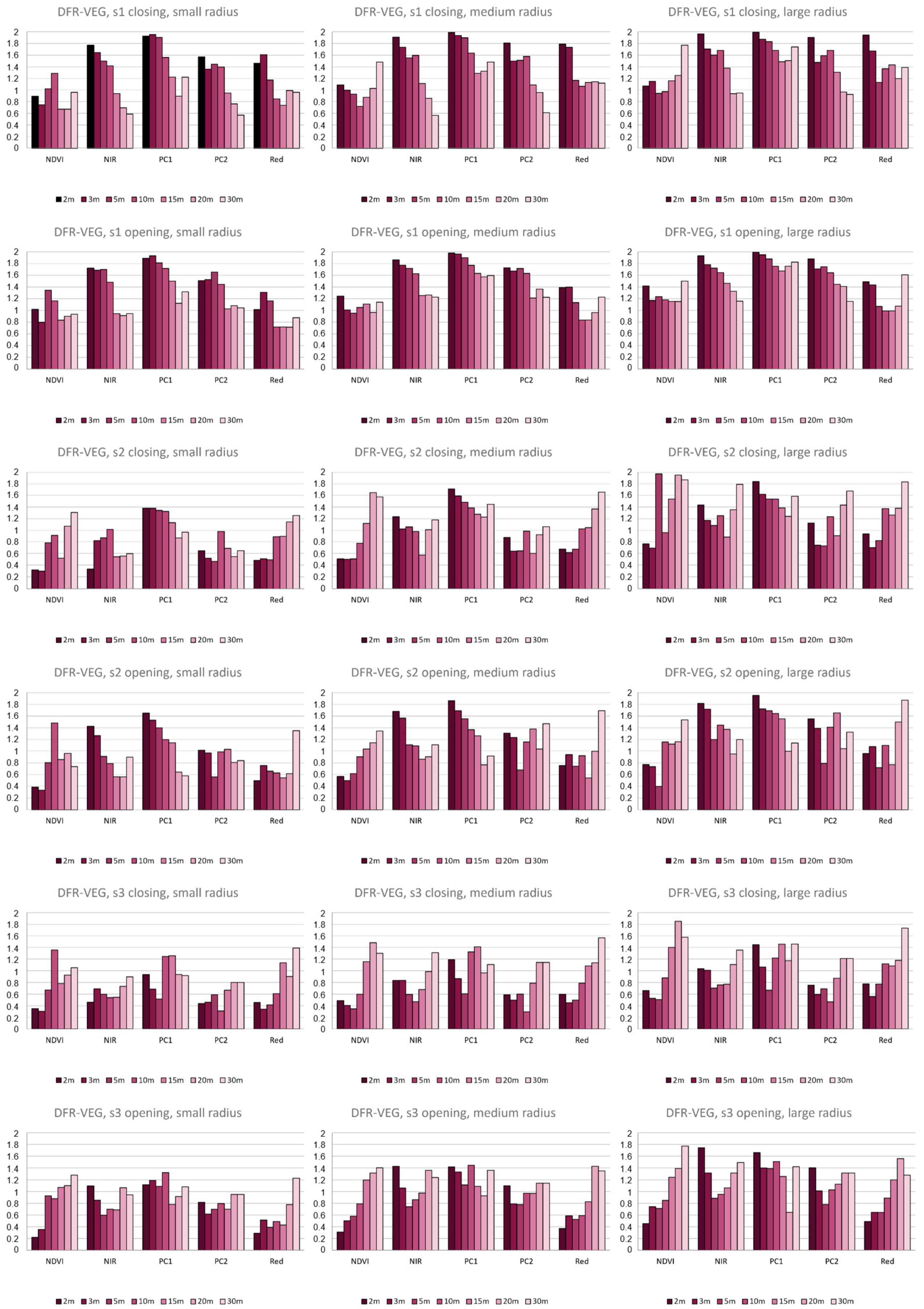
5.1. Deciduous Forest/Low Vegetation

The results obtained for this pair of classes are shown in Figure 4.

These two classes have relatively high spectral similarity but differ in texture, which is why textural analysis is particularly important for their separation. This is confirmed by the separability values obtained for the best combinations of analysis parameters. For these combinations J–M distance reaches the maximum values which shows that full separability is achieved only on the basis of texture data.

First of all, it is worth noting large differences between the results obtained for different types of source images. Clearly the best results were obtained for the first principal component (PCA1) image. Then, for the near-infrared (NIR) image and the second principal component (PCA2) image. Slightly worse results were obtained for the red channel (Red) image, while clearly the worst results were for the NDVI image. The NDVI is less useful for classification because the NDVI compensates for differences in illumination within an image, showing similar values for illuminated and shaded fragments of tree crowns and thus weakening the image of texture.

The importance of the pixel size for detecting texture is very clear. The best results were obtained for images with the smallest pixel (2 and 3 m), in particular granulometric maps with the lowest index value, which show a relatively small size of the texture grain allowing it to distinguish classes. Conversely, granulometric maps obtained with larger structuring elements (SEs) are characterized by lower separability of pixel values. On the other hand, in the case of images of lower resolution, an increase in separability can be observed which is associated with the increase in the size of analyzed elements. However, taking into account the size of a given structuring element (SE) in comparison with the size of the pixel (an SE of size 3 for an image having a pixel of 30 m equals a diameter of approx. 150 m), it can be stated that the result is related not to the texture of the object, but rather to the size of the object.

No significant differences were observed in relation to the different sizes of the neighborhoods. The results obtained for all three analyzed combinations were very similar. There were also no significant differences between the results obtained for the analysis based on opening or closing.

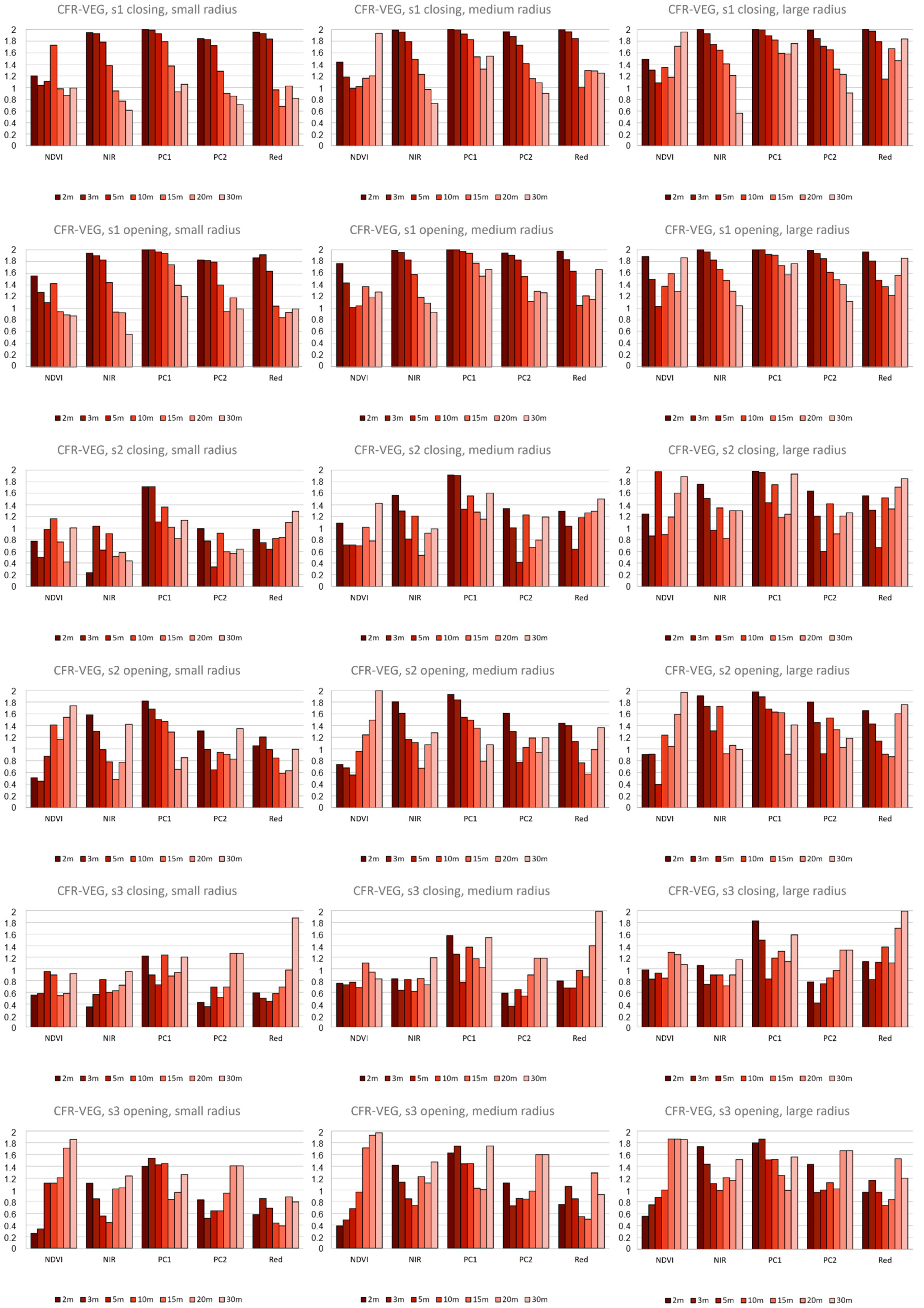
5.2. Coniferous Forest/Low Vegetation

The results obtained for this pair of classes are presented in Figure 5.

The texture of coniferous forests is characterized by less internal contrast than deciduous forests, which results from a lower contrast between illuminated and shaded tree crowns in the case of coniferous forests. Considering the low texture of low vegetation, one should expect less separability of the values obtained from the texture analysis. Indeed, the J–M distance values for this pair of classes are clearly lower than for the deciduous forest/low vegetation pair. Although it should be emphasized that for certain combinations of parameters, these values are still satisfactory from the perspective of separating classes.

As in the case of the deciduous forest/low vegetation class pair, the importance of the size of the structuring element (SE) can be clearly seen—granulometric maps obtained with the SE of the smallest size provide the best separability of compared classes, which shows that the texture grain itself is of small size.

Again, the impact of spatial resolution can be observed: in most analyzed cases, the class separability decreases roughly in proportion to the spatial resolution of the source images. This is best seen with NIR and PC2 source images, where this relationship is exceptionally well visible and stable. A much smaller decrease can be observed in the case of the analysis based on the PC1 image, which, as should be noted, again provides the best overall results, although its advantage is not as clear as in the case of the pair of deciduous forest/low vegetation classes.

The results obtained for operations based on opening and closing are very similar.

5.3. Coniferous Forest/Deciduous Forest

The results obtained for this pair of classes are presented in Figure 6.

The J–M distance values obtained for this pair of classes are relatively low and at the same time inconclusive. In the case of granulometric maps obtained with SE of size 1 an already observed relationship can be seen: separability decreases with the increase in the pixel size. It is worth emphasizing, however, that this effect is visible primarily in the PC1 image, for which the best results were obtained; in other images (NIR, PC2) the opposite effect can be observed, although it should be noted that the obtained values are low in this case. The positive effect of increasing the size of the neighborhood is noticeable (although this effect is not very significant).

Particularly interesting are the results obtained for granulometric maps with higher indices: the class separability was noted to increase largely when the pixel size was increased, and thus the opposite effect from what is observed in other cases. However, this effect is caused not by the texture resulting from properties of the analyzed classes, but rather by the structure of the object layout, which should not be generalized.

Once again, no significant differences were observed between the results obtained for images based on opening and closing.

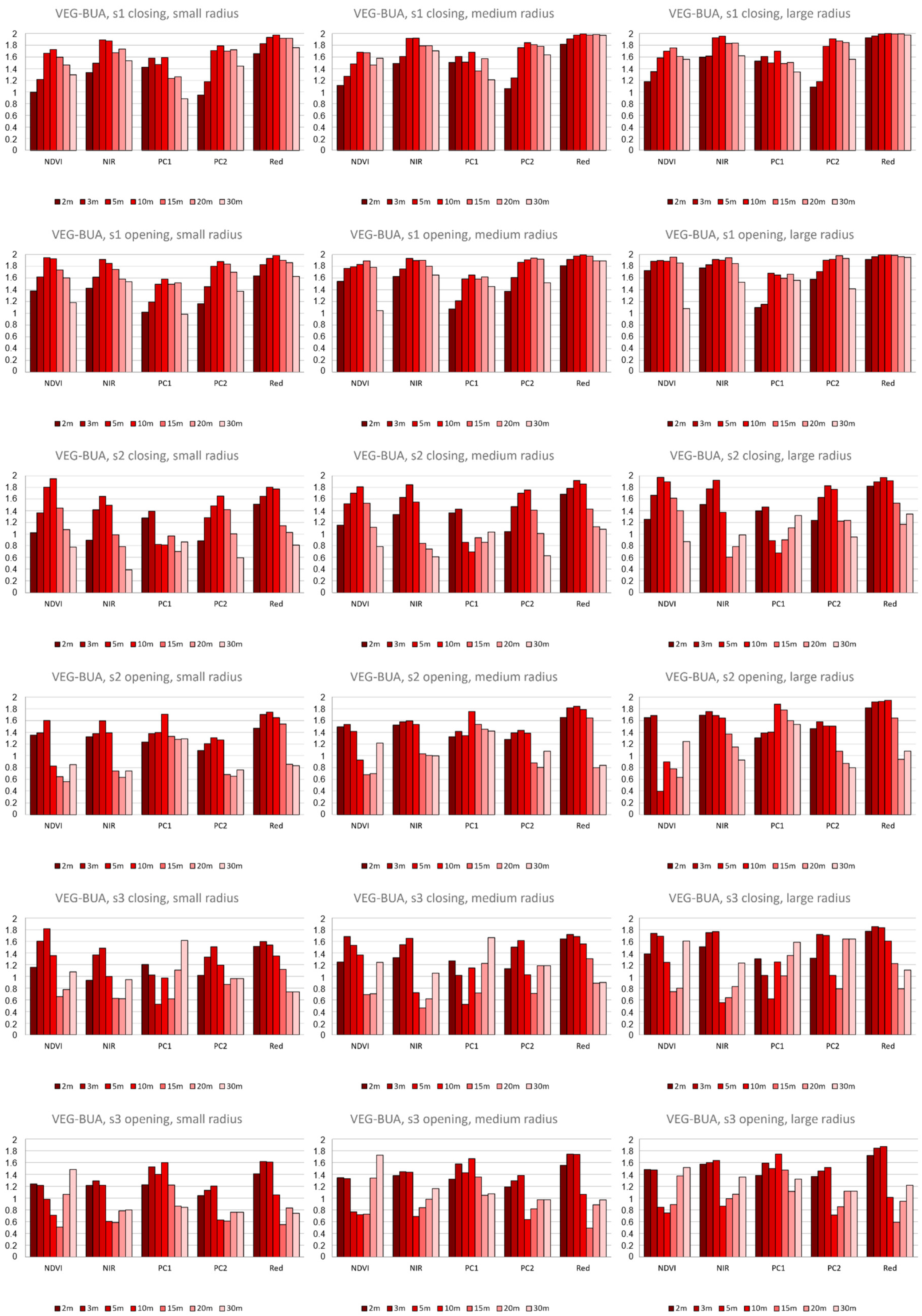
5.4. Low Vegetation/Built-Up Area

The results obtained for this pair of classes are shown in Figure 7.

For some combinations of texture analysis conditions, a very high separability of values for these two classes was obtained. The best results were obtained for the Red image, with better results obtained for a granulometric map generated with an SE of size 1 for lower resolution images than higher resolution images (with the best results achieved for images with pixels of 10 and 15 m). This can be explained by the size of the grain of the texture characteristic of the built-up areas class: in images with lower resolution the grain size calculated in pixels is obviously larger, which means that the information on the characteristic texture does not translate into values of granulometric maps obtained with SEs of the smallest size. Interestingly, however, while in lower-resolution images increasing the size of the structuring element (SE) brings a significant decrease in the separability between classes, an SE increase in higher-resolution images does not cause an increase in separability. Together with the observed positive impact of the size of the neighborhood on the effectiveness of the analysis (for images with the highest resolution), this indicates—as the cause of the observed phenomenon—the uneven nature of the texture of the built-up area. Due to this unevenness of texture a small neighborhood of the analysis produces varied results values, which translates into lower separability compared to other classes.

For the analysis based on closing, for images with the highest resolution and the index 2 (s2—size of the analyzed texture grain) worse results were obtained than for the analysis based on opening. Interestingly, this applies mainly to the analysis performed on NDVI, NIR and PC1. Considering that the operation based on opening analyzes the presence of bright texture elements, it can be concluded that this effect is related to the presence of bright objects (e.g., buildings, pavements, squares), allowing for a better distinction between the textures of both classes. It should be pointed out that in the discussed cases the effects obtained thanks to the opening—although better—are not fully satisfactory.

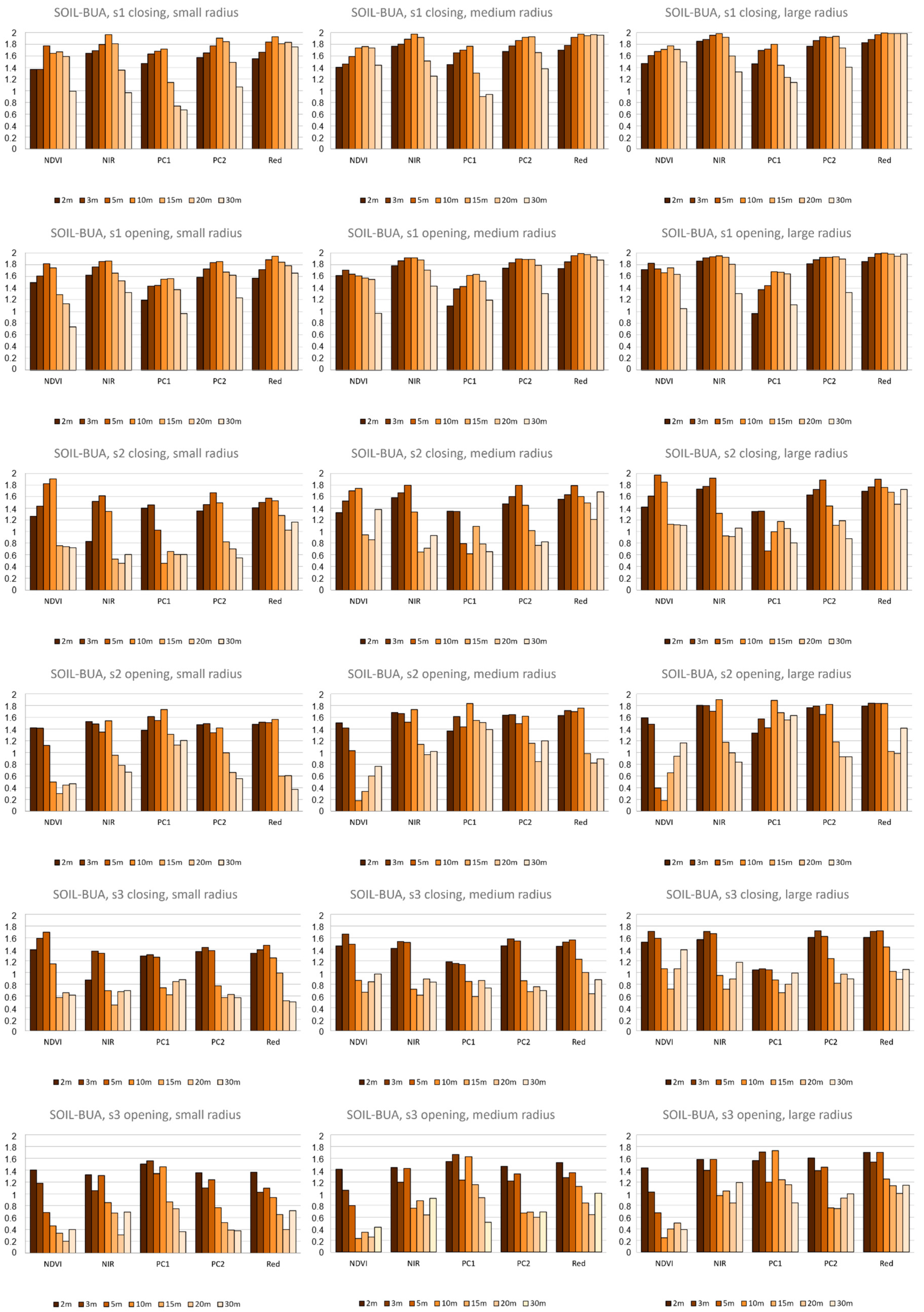
5.5. Bare Soil/Built-Up Area

The results obtained for this pair of classes are presented in Figure 8.

The results for this pair of classes are very similar to the results for the above-described pair of low vegetation and built-up area classes, with the difference that the observed separability is slightly lower. This similarity is understandable because the bare soil and low vegetation classes show similar weak texture, therefore the more distinctive texture of built-up areas is decisive. Hence, the best results were again obtained on the basis of the analysis of the red image (Red), for images with higher resolution (10 and 15 m), i.e., for the analysis carried out on the largest neighborhood (calculated in meters). Similarly, as in the previous low vegetation/built-up area class pair, the best results were obtained for granulometric maps generated with a structuring element (SE) of size 1; however, it is worth noting that while in the case of low vegetation the decrease in separability associated with increasing the SE size was relatively small, in the bare soil/built-up area pair discussed here this decrease is significant. This is caused by a greater heterogeneity of bare soils areas (linked, for example, with their varied humidity) which is revealed in maps obtained with larger SEs. This heterogeneity in combination with the high texture of built-up areas results in a reduction in the mutual class separability.

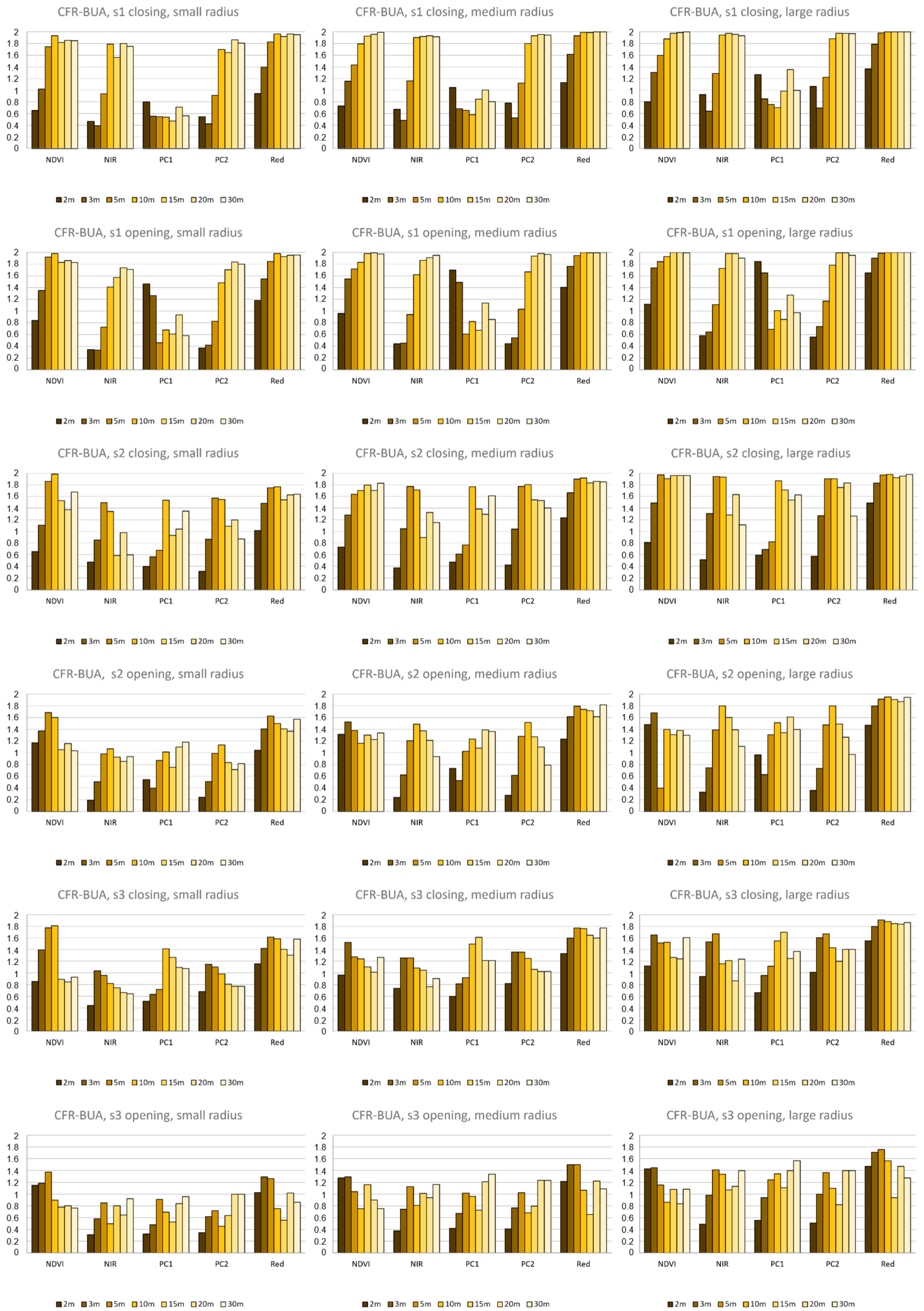
5.6. Coniferous Forest/Built-Up Area

The results obtained for this pair of classes are shown in Figure 9.

For this pair of classes, the results are similar to those described above for other pairs including built-up areas. This is primarily due to the previously described effect of separability increasing along with increasing the pixel size (in fact, along with increasing the area of analysis). As before, this probably results from the character of the texture of the built-up areas. However, compared to the previously described pairs that include built-up areas, in this pair the class separability is clearly lower, in particular in the case of images with higher resolution in which it is very low. This is due to the relatively strong texture of the coniferous forest class. It should be noted that in the case of the local analysis with the largest area of analysis, for the images with the largest pixel size full separability was obtained. The best results were obtained based on the analysis of the red image and (slightly worse) of the NDVI image. The results for NIR and PC2 followed (as in other cases the results for these two images are very similar). Once again, the worst results were obtained for the analysis of the PC1 image. In this case, however, the differences are quite significant: the results obtained for this image type indicate a very low separability of these two classes.

Again, the difference between the results obtained for the opening and closing for the analysis with the index s2 (the average size of the structuring element) can be seen. This time, however, better results were obtained based on closing. It should be noted, however, that we are dealing here with two classes with a distinct texture—hence the apparently different nature of the important features of this texture that distinguish these classes. The greater importance of closure (an operation analyzing the presence of dark texture elements) may indicate the importance of shadows of own forest areas.

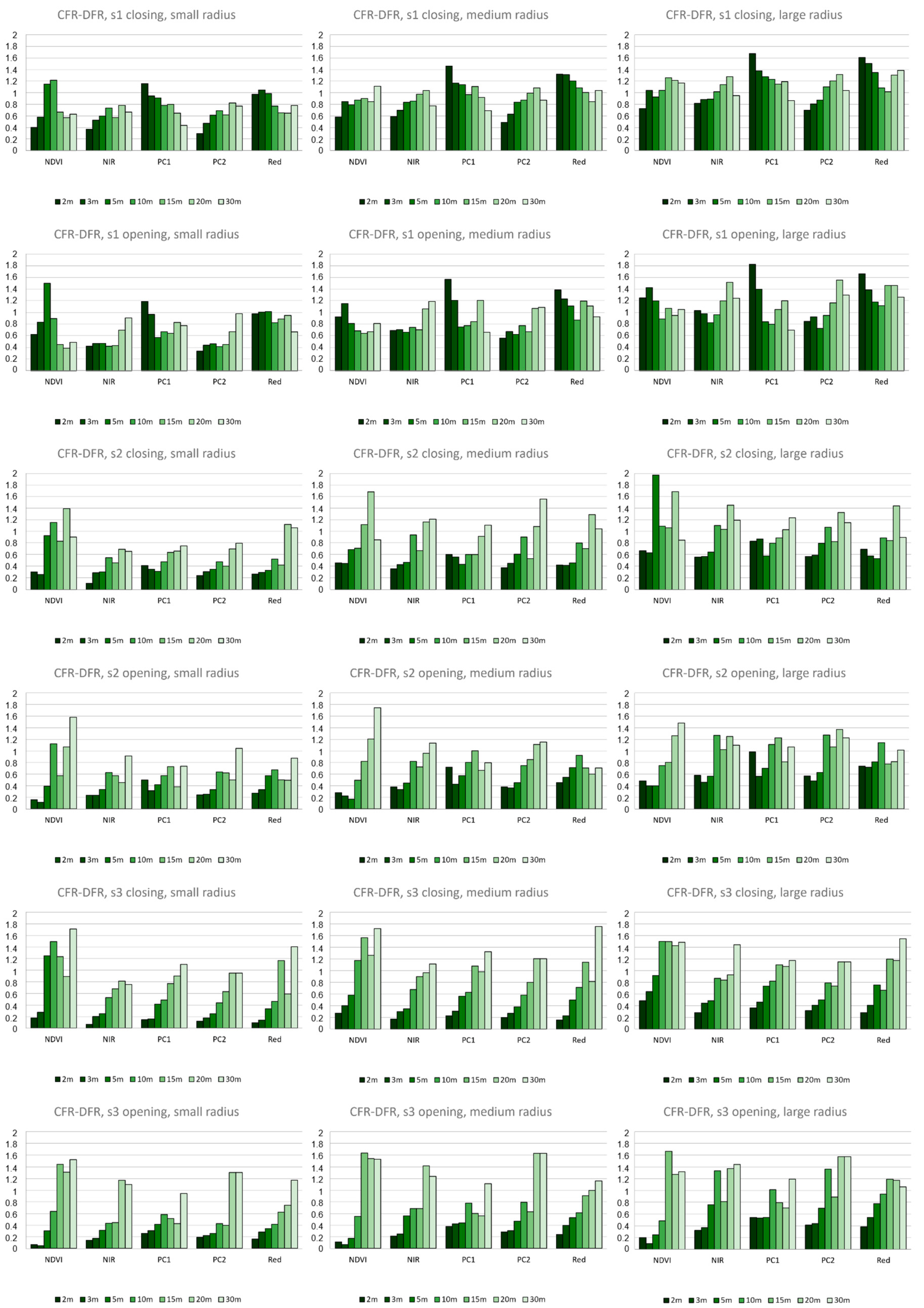
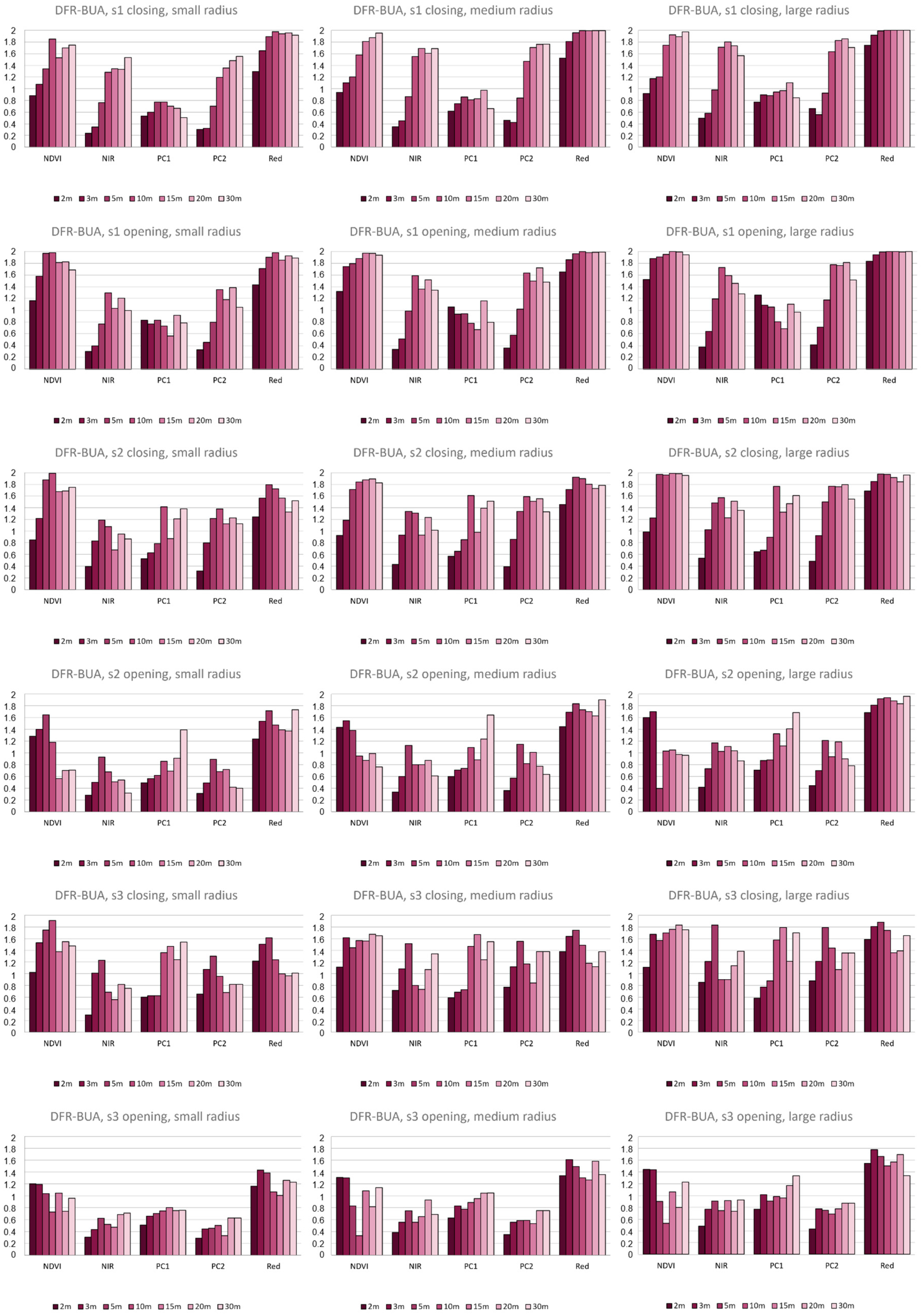
5.7. Deciduous Forest/Built-Up Areas

The results obtained for this pair of classes are presented in Figure 10.

The results obtained for this pair of classes are very similar to those obtained in the case of the pair of coniferous forest/built-up area classes, with the difference that here the separability values are slightly lower than in the previous case. This is probably due to the clearer texture of the deciduous forest, which to a certain extent makes this class similar to built-up areas also characterized by high texture.

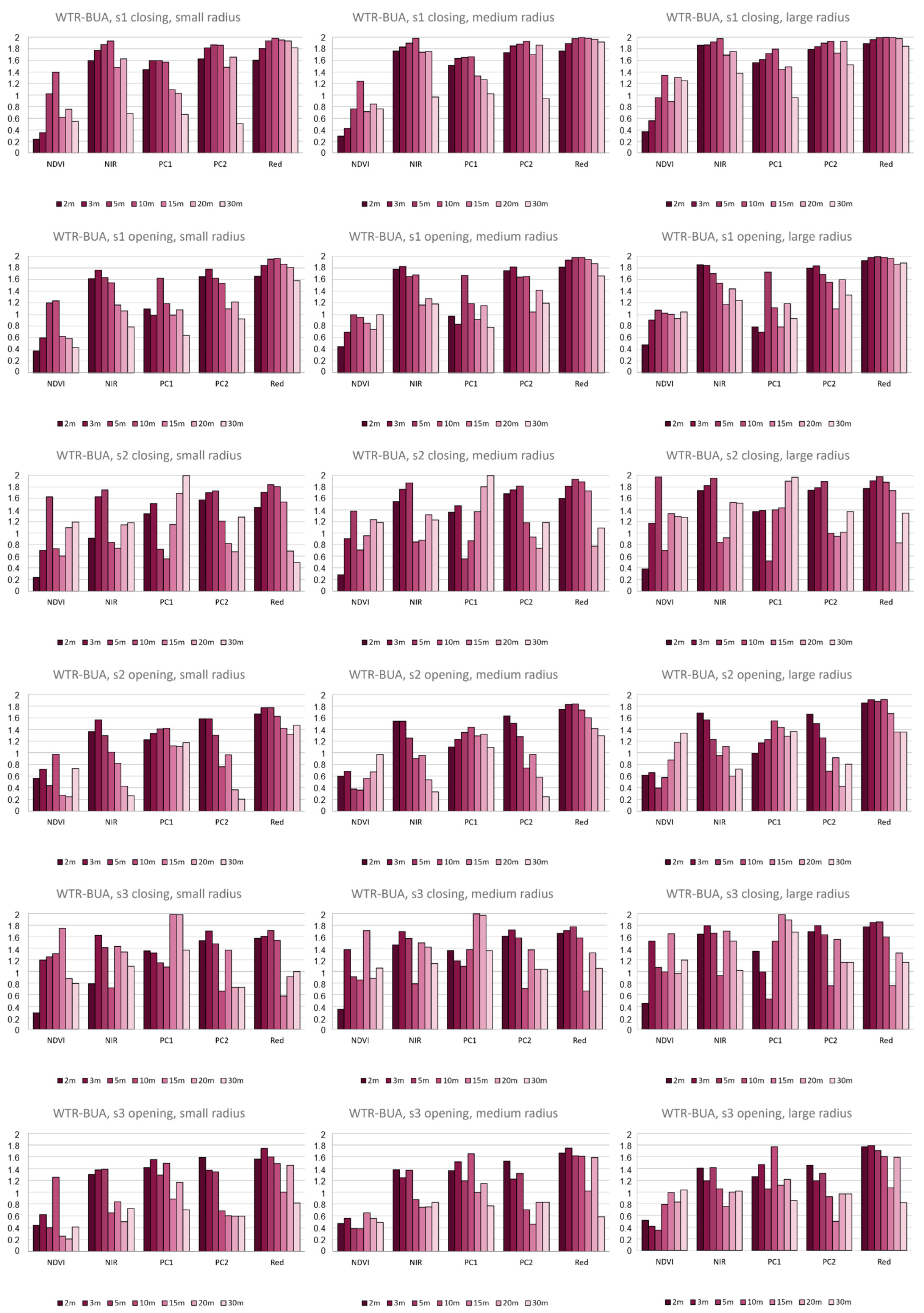
5.8. Water/Built-Up Areas

The results obtained for this pair of classes are shown in Figure 11.

The last of the compared pairs of classes shows similarity to the previously analyzed classes that include built-up areas. Due to the heterogeneous texture of built-up areas, images with the smallest pixel (and therefore effectively the smallest neighborhood of the analysis) show worse separability results. The best results were obtained for images with a pixel size of 10–15 m. Among the types of source images, the best results were obtained based on the red image, as in the case of other pairs of classes that include built-up areas. Again, the use of NIR and PC2 images leads to worse results (and very similar for both image types). The results are clearly worse than in the case of the red image, but in certain combinations of analysis conditions high values were still obtained indicating high separability. Unlike in previous cases, the worst results were obtained for the NDVI image. Better results were obtained for the analysis based on closure, which indicates a greater importance of dark elements in the texture of built-up areas in this case.

6. Conclusions

The obtained results showed that there is no single, universal combination of conditions of texture analysis which would be the best from the point of view of all classes (pairs of classes). Depending on the analyzed classes, the best results were obtained for different types of source images. However, the following generalization may be offered.

First of all, among the studied pairs of classes, those including built-up areas clearly stand out from other pairs. Better results were obtained for images with a larger pixel size (10–15 m), although it was not the size of the pixel itself that determined the effectiveness of the analysis but the associated size of the neighborhood. The results obtained for the class of built-up areas indicate, therefore, that the highest effectiveness was achieved for the analysis neighborhood having a larger radius. This is due to the widely varied texture of built-up areas (resulting from the presence of various elements: trees, buildings, their shadows, etc.), which, with a small area of analysis, results in a wide range of values, and, as a result, a difficulty in distinguishing these values from the values obtained for other LULC classes. Interestingly, the best results for this class were obtained on the basis of the products of red image analysis, which is also exceptional compared to other pairs of LULC classes. In summary, for separating built-up areas the best results were obtained based on the texture analysis of Red image with 10–15 m resolution with a large analysis neighborhood.

For the remaining pairs of classes, however, the relationship between the effectiveness of texture analysis and the spatial resolution of the image is unambiguous: images with higher resolution enable a more effective texture analysis. The effectiveness of the analysis may vary, but in all cases—with the exception of a pair of forest classes (deciduous forest/coniferous forest)—full separability of the analyzed test fields was obtained for images with the smallest pixel. The specific relationship between image resolution and effectiveness of the analysis varies depending on the pair of images analyzed, but it can be concluded that the effectiveness clearly decreases for images having a pixel size of 10–15 m. Moreover, the best image to be used for the studied classes as the basis for textural analysis (except for the class of built-up areas) is clearly the first main component (PC1) image. The analysis carried out on the basis of this type of image allowed us to obtain the greatest separability of pixel values for different compared classes. Interestingly, the worst image in terms of separability was the red image, which, in turn, offered the highest separability when the class of built-up areas was compared with other classes.

In almost all the analyzed cases it can be noticed that the best results were obtained on the basis of granulometric maps generated with SEs of the smallest sizes, even in the case of the highest resolution images. This indicates a small size of the grain of the texture characteristic of individual classes. It can also be seen that the class separability decreases in granulometric maps obtained with larger SEs. However, this does not necessarily show the uselessness of multi-scale analysis, as even partially useful data can be a valuable addition to the data set (in certain cases, granulometric maps obtained with higher SE sizes also produced decent separability).

In conclusion, for separating most of the classes, except for built-up areas, the best results were obtained based on the analysis of PC1 image of the highest resolution (2–5 m, with a noticeable decrease in the analysis effectiveness for images with 10 m and lower resolution) and the smallest size of the structuring element (size 1). No significant impact of the neighborhood size on the effectiveness of the analysis was observed.

The conducted analyses have not allowed us to conclude that either of the two types of granulometric analysis (opening- or closing-based) is more effective. Naturally, in certain cases, differences can be observed between the results of the analysis based on opening and closing, which is understandable due to the fact that in various cases light or dark grains of texture may be of different sizes, which may lead to higher or lower separability. However, no significant, constant differences were observed. For greater effectiveness of texture analysis, it may thus be useful to take products of both types of granulometric analysis as the basis for the processing.

The conducted research relates to the generally understood texture, as it is “seen” by granulometric analysis. However, since there is no unambiguous mathematical definition of texture, different methods may estimate it differently. While it can be expected that the general trend would be similar in most cases, the analysis of the impact of the features studied here on selected texture aspects represented by selected GLCM metrics may be an interesting field of further exploration.