Article

Large-Scale Impervious Surface Area Mapping and Pattern Evolution of the Yellow River Delta Using Sentinel-1/2 on the GEE

1
School of Surveying and Geo-Informatics, Shandong Jianzhu University, Jinan 250101, China
2
College of Applied Arts and Sciences, Beijing Union University, Beijing 100191, China
*
Author to whom correspondence should be addressed.
Remote Sens. 2023, 15(1), 136; https://doi.org/10.3390/rs15010136
Submission received: 6 November 2022 / Revised: 21 December 2022 / Accepted: 23 December 2022 / Published: 26 December 2022

Abstract

:
The ecological environment of Yellow River Delta High-efficiency Ecological Economic Zone (YRDHEEZ) is adjacent to the Bohai Sea. The unique geographical location makes it highly sensitive to anthropogenic disturbances. As an important land surface biophysical parameter, the impervious surface area (ISA) can characterize the level of urbanization and measure the intensity of human activities, and hence, the timely understanding of ISA dynamic changes is of great significance to protect the ecological safety of the YRDHEEZ. Based on the multi-source and multi-modal Sentinel-1/2 remotely sensed data provided by Google Earth Engine (GEE) cloud computing platform, this study developed a novel approach for the extraction of time-series ISA in the YRDHEEZ through a combination of random forest algorithm and numerous representative features extracted from Sentinel-1/2. Subsequently, we revealed the pattern of the ISA spatial-temporal evolution in this region over the past five years. The results demonstrated that the proposed method has good performance with an average overall accuracy of 94.84% and an average kappa coefficient of 0.9393, which verified the feasibility of the proposed method for large-scale ISA mapping with 10 m. Spatial-temporal evolution analysis revealed that the ISA of the YRDHEEZ decreased from 5211.39 km2 in 2018 to 5147.02 km2 in 2022 with an average rate of −16.09 km2/year in the last 5 years, suggesting that the ISA of YRDHEEZ has decreased while its overall pattern was not significantly changed over time. The presented workflow can provide a reference for large-scale ISA mapping and its evolution analysis, especially in regions on estuarine deltas.

1. Introduction

Impervious surface area (ISA) refers to materials that can prevent the infiltration of surface water into soil, such as concrete roads, buildings, car parks, etc. [1] It has an important impact on the ecological environment quality of the region, which is prone to resulting in urban heat island effect and flood disasters [2]. The research conducted on ISA can underpin our understanding of the regional urbanization process [3,4,5]. Furthermore, ISA data, especially long time-series, is also an indispensable data reference for formulating a sustainable urban development plan [6,7].
With the advance of remote sensing technology and machine learning, multitudes of studies on the extraction of the ISA have been conducted using remotely sensed data. As early as 2003, Murray et al. estimated the spatial distribution of the ISA based on Landsat images using the VIS model [8]. Subsequently, Lu et al. explored the extraction of the ISA with a multi-resolution remote sensing image in 2014 [9], and from then on, multisource images began to be extensively applied to ISA mapping. Piyoosh et al. developed a novel urban index called NRUI for identifying urban areas, and their experimental result revealed that NRUI was able to effectively discriminate urban area from soil [10]. In recent years, Shrestha Binita et al. combined Sentinel-1/2 data to yield ISA spatial distribution data [11], which provided new perspective on ISA mapping through synergic use of optical and radar data. Due to its powerful data fitting capabilities, machine learning is extensively adopted for land use/land cover mapping in remote sensing fields. For example, Liu et al. estimated the fraction of the ISA using random forest regression in the Nansi Lake region [12]. Liu et al. presented a method for extracting ISA information based on combined kernel support vector regression [13]. Zhang et al. developed an ISA mapping method through combining multi-temporal Landsat data with a decision tree algorithm over the Pearl River Delta area [14]. Additionally, a few studies have been performed for the investigation of ISA in the Yellow River Delta through reviews. Liu et al. obtained the ISA distribution data in Dongying City in 2019 by integrating Sentinel-1/2 remotely sensed data with a random forest approach, which exhibited the potential of multi-source multi-modal data to produce ISA information [15]. The research on the impact of the expansion of the ISA on the ecological environment has been conducted with Bohai Bay Rim (covering Dongying City and Binzhou City) as the study area [16]. Currently, the major approach to extract the ISA focused on the combination of optical remotely sensed data and spectral indices generated with a calculation among different bands [17,18].
The optical remote sensing images collected the reflective information of ground objects, which are inevitably affected by natural weather, such as atmospheric conditions, clouds, and so on. Due to the existence of spectral confusion between different types of ground objects, the accuracy of ISA data derived from optical data was typically unsatisfactory [19]. Synthetic aperture radar (SAR), characterized by its features of all-day, all-weather, and strong penetration [20], can acquire reliable periodic data without the influence of natural weather, which can effectively compensate for the drawbacks of optical remote sensing images [21,22] and improve the extraction accuracy of the ISA [23,24]. Several studies have demonstrated the feasibility and potential of synthetic aperture radar data for ISA extraction [25,26]. Due to the extensive coverage, the categories of landscape in the YRDHEEZ are complex and diverse, which poses a great challenge to the extraction of the ISA in this region when only optical images are involved. The research performed by Lin et al. has verified the feasibility of fusing multi-source and multi-modal optical and radar images for mapping ISA [27]. Furthermore, most of the previous studies commonly used single-polarized SAR images for ISA mapping, with the exception of Zhang’s study on which dual-polarized SAR images were utilized to produce ISA data [28]. Overall, the aforementioned studies demonstrated that incorporating optical multispectral images and dual-polarized SAR images show great potential for generating l ISA data.
Although multi-source multimodal images have achieved excellent performance in ISA mapping, it inevitably extended the data processing period to a large extent due to limited computing power of local computers. Confronted with the above challenges, the remote sensing cloud computing platform provided by Google Earth Engine (GEE) gains increasing attention. The availability of millions of cloud servers makes GEE cloud computing platform efficiently process massive remote sensing images data without relying on local computer resources. Meanwhile, the GEE platform stores vast free remote sensing images sets that have been preprocessed worldwide, such as Sentinel and Landsat satellite images. Thus, the GEE platform reduced the cycle of data processing and the cost of data processing [29]. In the study conducted by Haifa et al. [30] and Wang et al. [31], the application status and potential of GEE cloud computing platform were comprehensively reviewed. Nowadays, with the support of GEE cloud computing platform, the research on ISA extraction has made great progress [23,32,33].
Yellow River Delta High-efficiency Ecological Economic Zone (YRDHEEZ) occupies massive lands, abundant natural resources, and unique ecological environment, on account of which the Chinese government attaches great importance to the development of the region. The unique geographical location adjacent to the Bohai Sea makes its ecological environment considerably fragile and highly sensitive to anthropogenic disturbances. As an important land surface biophysical parameter, the ISA can characterize the level of urbanization and measure the intensity of human activities, and hence, the timely understanding of ISA spatial-temporal evolution characteristic is of great significance to maintain the ecological safety of the YRDHEEZ [7]. However, literature reviews revealed that few studies combined Sentinel-1/2 with random forest algorithm to delineate the annual ISA at a scale of 10 m and analyze its spatial-temporal pattern for this region in recent years.
In this study, we aim to generate large-scale annual continuous ISA data with 10m in the YRDHEEZ ranging from 2018 to 2022 using a random forest classifier through the combination of Sentinel-1 synthetic aperture radar (SAR) images and Sentinel-2 optical multispectral (MSI) images provided by GEE and subsequently analyze the spatiotemporal evolution pattern of the ISA in the last five years. More specifically, this study aimed (i) to determine whether ISA mapping accuracy was improved when Sentinel-1 SAR backscattering features, spectral indices, and GLCM texture features from Sentinel-2 were synergistically used; (ii) to understand what the ISA spatial-temporal evolution characteristics were in the YRDHEEZ during study period; and (iii) to attempt to provide beneficial suggestions for the protection of ecological environment and sustainable development of the YRDHEEZ.

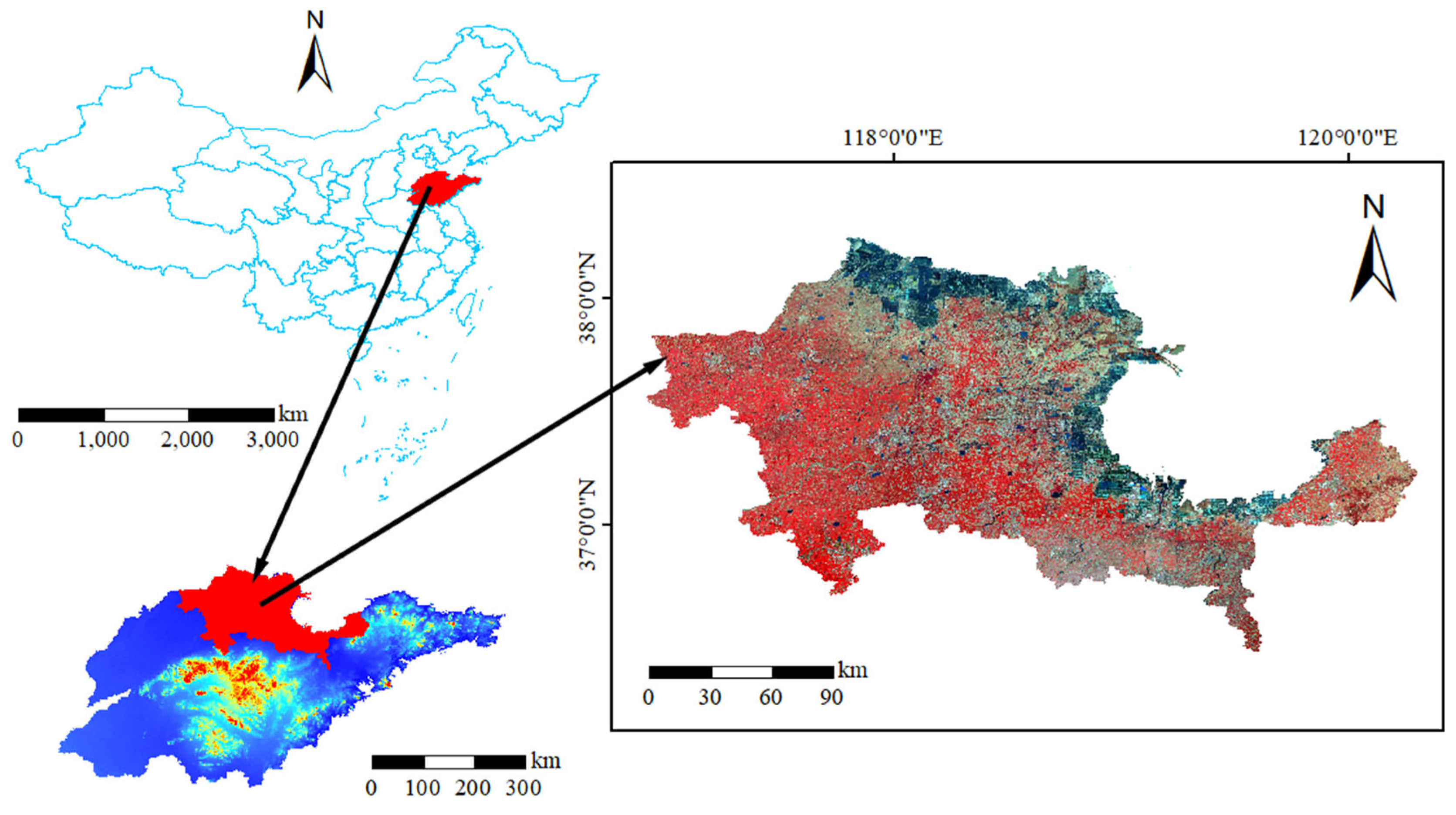
2. Study Area and Datasets

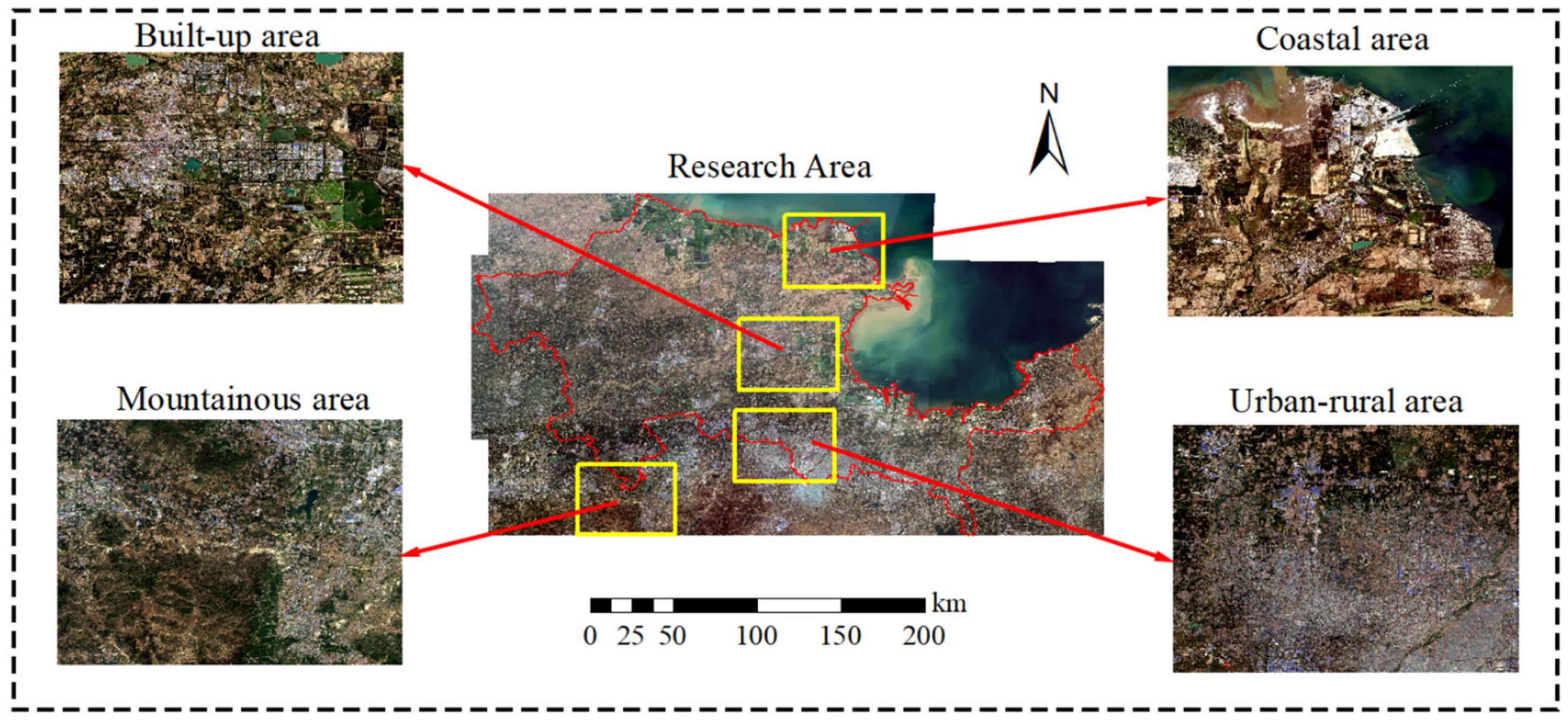
2.1. Study Area Overview

As one of the three major estuarine deltas in China, the Yellow River Delta have the most extensive wetland ecosystem in warm temperate zone of China [34]. Its unique geographical location makes ecological environment of the Yellow River Delta extremely fragile and is easily subjected to disturbance from anthropogenic activities. [35]. Therefore, the Yellow River Delta region holds a unique strategic location [36,37] from the perspective of regional ecology safety. The YRDHEEZ is the region planned by China State Council, which contains wholly the Yellow River Delta and is located at 116° E~120° E and 36° N~38° N (Figure 1). The YRDHEEZ consisted of a total of 19 counties or districts with the total area of 26,500 square kilometers, including Dongying City, Binzhou City, DeZhou City, and so on. For a long time, China has attached great importance to the sustainable development of the YRDHEEZ due to its rich natural resources and important geographical location.

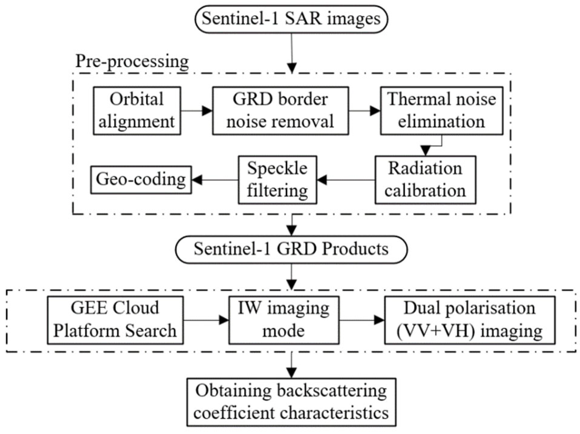
2.2. Data Sources and Pre-Processing
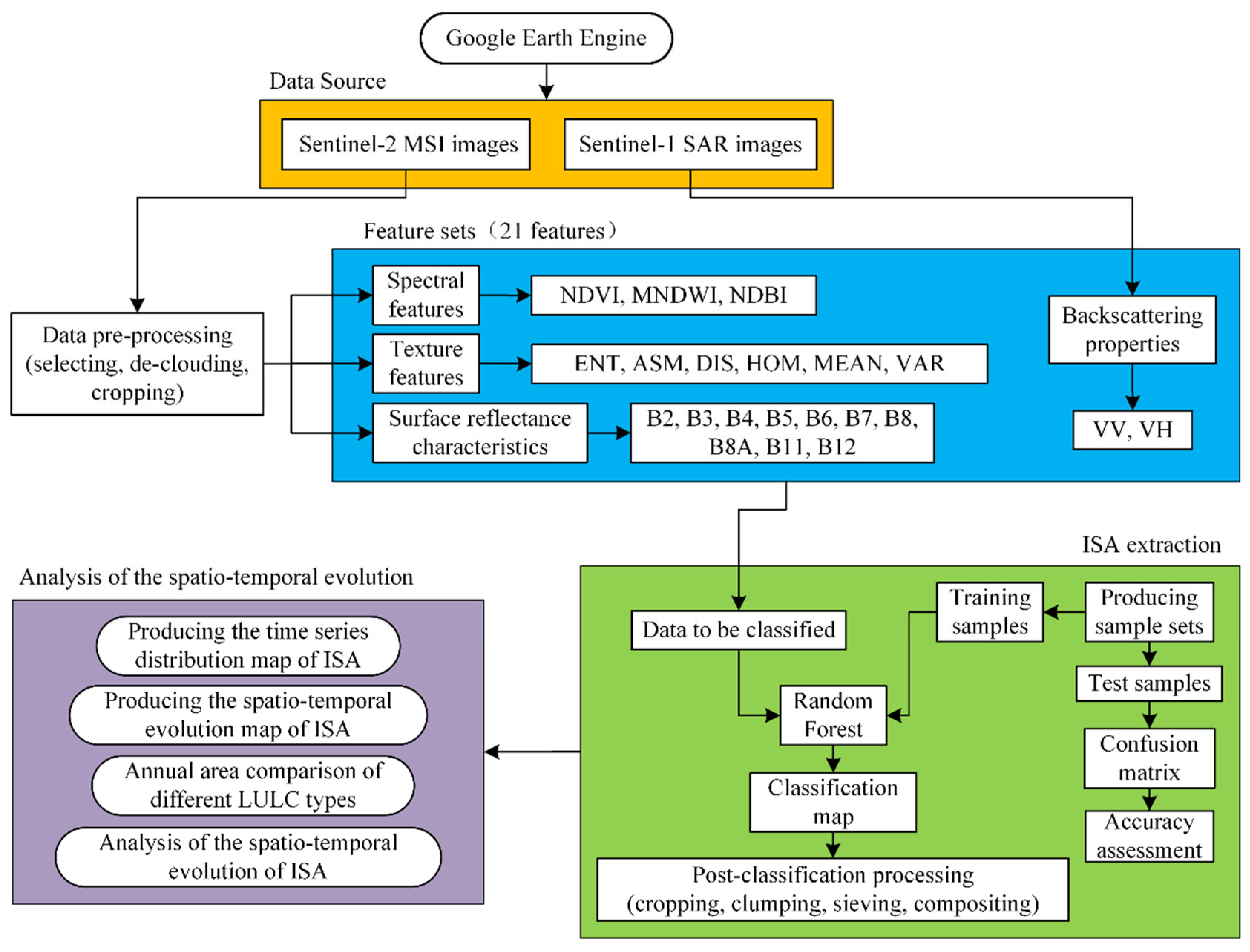
The remote sensing data used in this study was derived from Sentinel series of ESA ‘Copernicus Plan’ satellites. In order to accurately the identify different land use/land cover types in the YRDHEEZ, this study selected Sentinel-2 multi-spectral (MSI) images with cloud coverage less than 5 % and Sentinel-1 synthetic aperture radar (SAR) data (Table 1) in the past five years to extract annual continuous time-series ISA spatial distribution data. The GEE cloud platform stores Sentinel-1 satellite images that has undergone the following pre-processing steps: (i) Orbit correction; (ii) Boundary noise removal, including the removal of invalid data; (iii) Thermal noise removal; (iv) Radiometric calibration; and (v) Orthorectification and Sentinel-2 satellite image data with radiometric calibration and geometric and atmospheric corrections. For the satellite images of Sentinel-1/2, all the data pre-processing steps can be completed with a simple image filtering and de-clouding process in the GEE cloud computing platform, which greatly reduces the data processing cycle.

3. Methods

3.1. Methodology Flow

The ISA extraction based on multi-source and multi-modal Sentinel-1/2 imagery is illustrated in Figure 2 and mainly summarized in the following five steps. (i) Data pre-processing involves collecting Sentinel-1/2 images with less than 5% cloud coverage in the last 5 years and conducting cloud removal and cropping for the data; (ii) the building classification feature set involves (a) the extraction of 3 spectral indices (NDVI, NDBI, MNDWI) and 6 GLCM texture features with weak correlation using Sentinel-2 multispectral images, (b) the production of 2 backscattering coefficient features (VH and VV) from Sentinel-1 SAR images, and (c) combining Sentinel-2 surface reflectance features, spectral indices, backscattering coefficient, and GLCM textures to form feature set for classification (21 features). (iii) Collecting samples give a wide coverage of the study area, hence four representative areas are selected as the samples collection area, and the sample set is made by visual interpretation method combined with the historical images of the Map World. Subsequently, approximately 70% of the samples are randomly selected to construct the training set while the remaining samples constituted the test set. (iv) The ISA extraction and accuracy assessment: a random forest classifier was adopted for ISA extraction and a confusion matrix was utilized to test the accuracy of classification results. Five experiments based on different classifiers and different sets of features are also carried out for comparison to verify the superiority of the designed workflow. (v) For the spatial–temporal evolution analysis of the ISA, evolutionary mapping and an analysis on the ISA were conducted using time-series of the ISA in the YRDHEEZ over the past five years.
In this study, we combined dual-side strategy (cloud platform and local computation) for ISA extraction. First, the GEE cloud platform was used for image pre-processing, feature extraction, and the classification of large computer resources as well as high time consumption. The local computer was employed for samples collecting, mapping revision, and so on. The strategy was beneficial to make full use of cloud storage and computing capabilities while greatly avoiding the drawbacks of GEE.

3.2. Feature Extraction

Considering the unique topography of the Yellow River Delta and the complex and diverse types of ground objects in this region, our study adopts a feature-level fusion strategy for multisource data integration to better distinguish different land use/land cover and decrease the spectral confusion between different land use/land cover and the “salt and pepper” phenomenon. A total of 21 features were calculated and fed to the classifier for ISA Mapping, including 3 spectral index features (NDVI, NDBI, MNDWI), 6 GLCM texture features, 10 land surface reflectance features, and 2 backscattering features.

3.2.1. Spectral Indices Feature

Early studies indicated that combining spectral indices features is conductive to improvement of accuracy in ISA mapping [38,39]. In this study, the following three spectral indices features were calculated, including the Normalized Difference Vegetation Index (NDVI), which can highlight vegetated land [40]; the Modified Normalized Difference Water Index (MNDWI), which has a good effect on distinguishing water bodies from land use/cover [41]; and the Normalized Difference Built-up Index (NDBI), which has a significant effect on the extraction of ISA [42]. The calculation formulas are as follows.
N D V I = ρ N I R ρ R E D ρ N I R + ρ R E D
M N D W I = ρ G R E E N ρ S W I R ρ G R E E N + ρ S W I R
N D B I = ρ S W I R ρ N I R ρ S W I R + ρ N I R
where ρ N I R , ρ R E D , ρ G R E E N , and ρ S W I R correspond to the B8 (near infrared band), B4 (red band), B3 (green band), and B11 (short-wave infrared band) of the Sentinel-2 images, respectively.

3.2.2. Textural Features

Related studies have shown that the addition of texture features can improve accuracy of ISA mapping [43,44]. Referring to the research of Szantoi et al. [45], this study selected the following six second-order texture features with minimal correlation for classification to calculate including Entropy (ENT), Angular Second Moment (ASM), Dissimilarity (DIS), Homogeneity (HOM), Mean (MEAN), and Variance (VAR) [43]. Their calculation formulas are as follows.
E N T = x = 0 n - 1 y = 0 n - 1 R ( x , y ) × ln ( R ( x , y ) )
A S M = x = 0 n - 1 y = 0 n - 1 R ( x , y ) 2
D I S = x = 0 n - 1 y = 0 n - 1 R ( x , y ) × | x y |
H O M = x = 0 n - 1 y = 0 n - 1 R ( x , y ) 1 + ( x y ) 2
M E A N x = x = 0 n - 1 y = 0 n - 1 x × R ( x , y )
V A R x = x = 0 n - 1 y = 0 n - 1 R ( x , y ) × ( x M E A N x ) 2
where R represents an nth-order co-occurrence matrix, n represents the number of grey levels, x and y represent the rank coordinates, and R (x, y) denotes the normalized grey-level value in cell x,y of the co-occurrence matrix.
Due to the strong correlation between different spectral bands, this study only utilized a single red band for deriving textural features through GEE platform. In order to determine the optimal moving window size for texture calculation, trial-and-error experiments were performed, and finally, a moving window size of 5 × 5 was used, under which a high accuracy was obtained.

3.2.3. Backscattering Features

Previous studies have shown that the backscattering coefficient properties have a significant optimization effect on the ISA extraction [15]. In this study, the dual-polarized (VV + VH) bands in IW imaging mode are selected based on the Sentinel-1 GRD product, and the above two bands are used as the backscattering coefficient feature bands to improve the extraction of ISA. The calculation process of backscattering is shown in Figure 3.
In the terrestrial model, when ρ 0 ( α ) is less than 2, the backscattering coefficient model can be expressed by the following equation.
ρ 0 ( α ) = K cos α
where α is the angle of incidence and ρ 0 ( α ) is the representative backscattering coefficient.

3.3. Samples Selection

According to the actual situation of the study area and document reviews, the land use/cover types of the study area were categorized into 10 categories: ISA (built-up, rural settlement), water area, plastic greenhouses, cropland (fallow land, arable land), saltern, tidal flat, woodland and grassland, and unused land. Through field survey, Google Earth imagery, and other high-resolution images, a total of approximately 5000 mutually independent samples were collected, and the number of samples and the description for each class are shown in Table 2. Among the collected samples, approximately 70 % of the total samples were randomly selected as the training samples, and the remaining approximately 30 % were used for the test samples.
The YRDHEEZ occupied a vast area, so numerous Sentinel-1/2 images were required for covering it entirely. In order to reduce the data processing cycle and make full use of computer resources, four representative areas were selected for sample collection in this study. Figure 4 shows four representative sample areas (mountainous area, urban-rural combination area, built-up area and coastal area) selected from the images acquired on 2022.

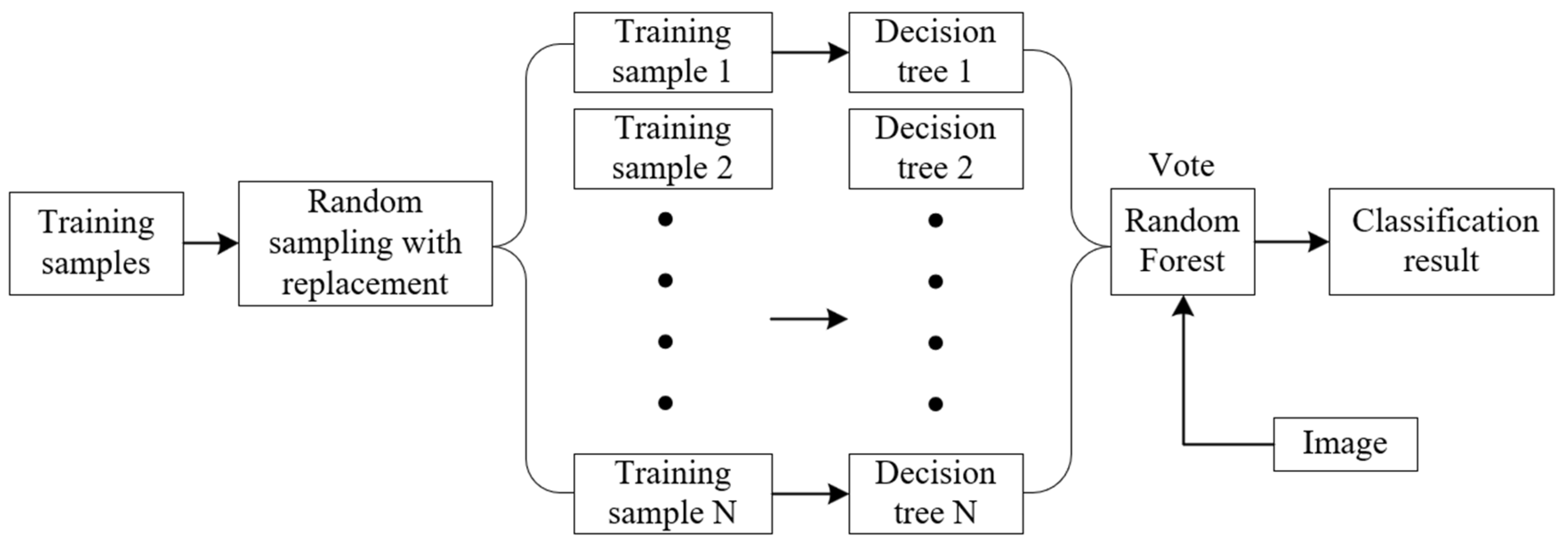
3.4. Random Forest Algorithm

The random forest (RF) algorithm was proposed by Breiman in 2001 [46], and the core of the RF is to create multitudes of decision trees that form the “forest” [46]. The principle of the RF is shown in Figure 5, and the detailed steps consist of the following four parts. (a) A randomly selected 2/3 of the samples with replacement are used to build N training sample sets, and the remaining 1/3 of the samples are used to test the performance of the corresponding decision trees, which is known as out-of-bag estimation (OOB) data. (b) N decision trees are built based on the training sample sets; (c) all nodes of the N decision trees utilize T features randomly selected from the classification feature set to carry out the split growth and select the optimal branch based on the principle of minimum Gini index [47]. (d) Based on ensemble learning theory to count the classification results predicted by each decision tree, the final land use/land cover type is determined by voting.
In random forest classification, only two parameters, ntree (number of decision trees) and mty (number of predictor variables) need to be set. After several experiments, it is found that the OOB error tends to be stable when the selected ntree reaches 500.

3.5. Accuracy Assessment

Accuracy assessment is an indispensable step in the workflow of ISA mapping. In order to verify the reliability of the classification result, a hybrid qualitatively visual inspection and quantitative metrics were adopted. Visual inspection was utilized to evaluate the visual effects of the classification results from a subjective view. Quantitative metrics included overall accuracy (OA), Kappa coefficient (κ), user’s accuracy (UA), and producer’s accuracy (PA), and all the four metrics can be calculated through a confusion matrix that can be yielded by independent test samples. In this study, the test samples were derived from a field survey, Google Earth imagery, and other high-resolution images. The mathematical expressions of the four metrics are as follows.
O A = i = 1 C n i i / N
κ = [ N i = 1 C n i i i = 1 C ( n i + n + i ) ] / [ N 2 i = 1 C ( n i + n + i ) ]
U A = i = 1 C n + i / N
P A = i = 1 C n i + / N
where C represents the number of land use/land cover types. In this study, C is equal to 10; N stands for the total number of test samples; nii represents the number of samples located in the main diagonal of the confusion matrix; ni+ is the number of ground truths for each type; n+i is the number of the i-th type of the predicted result.

4. Results

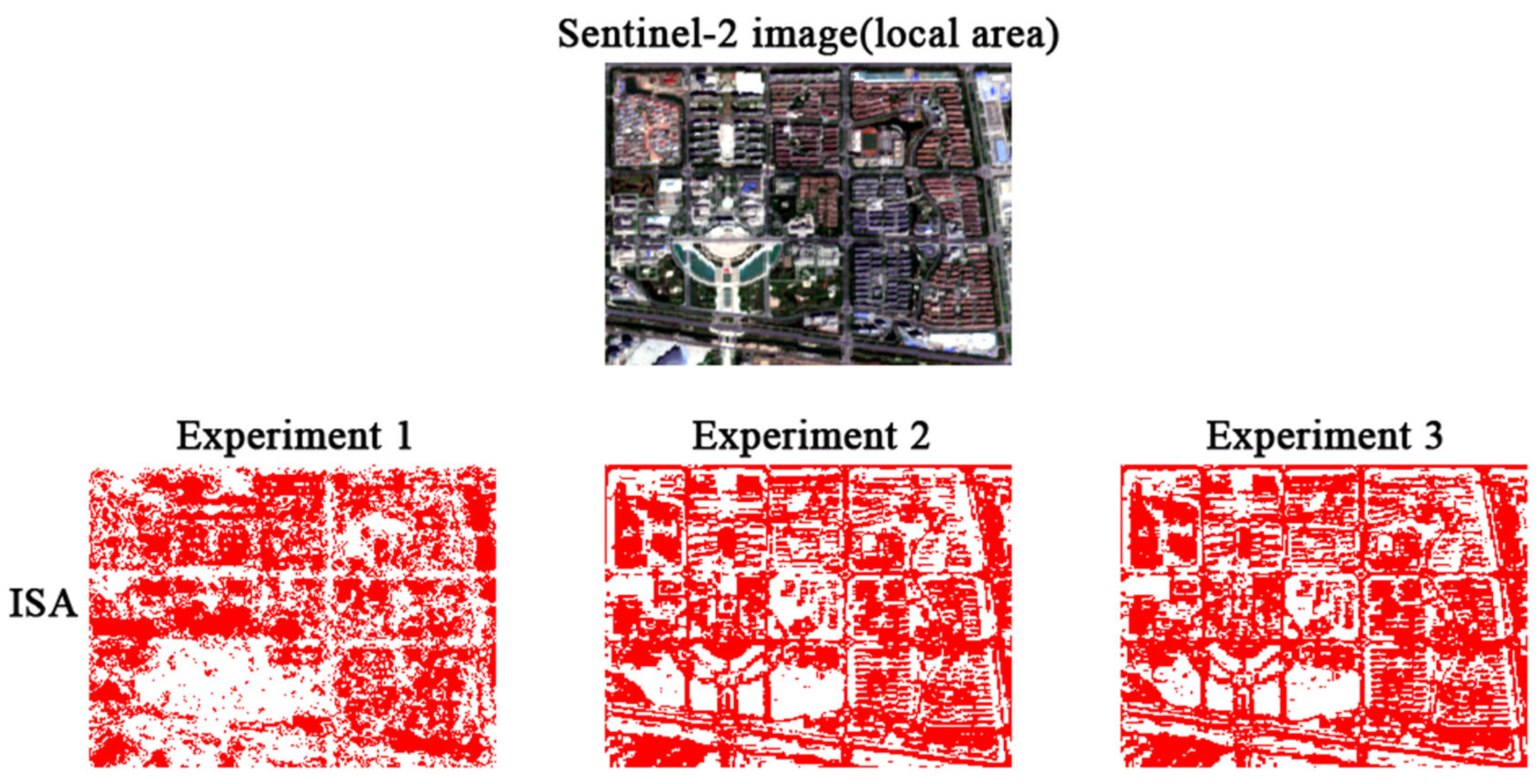
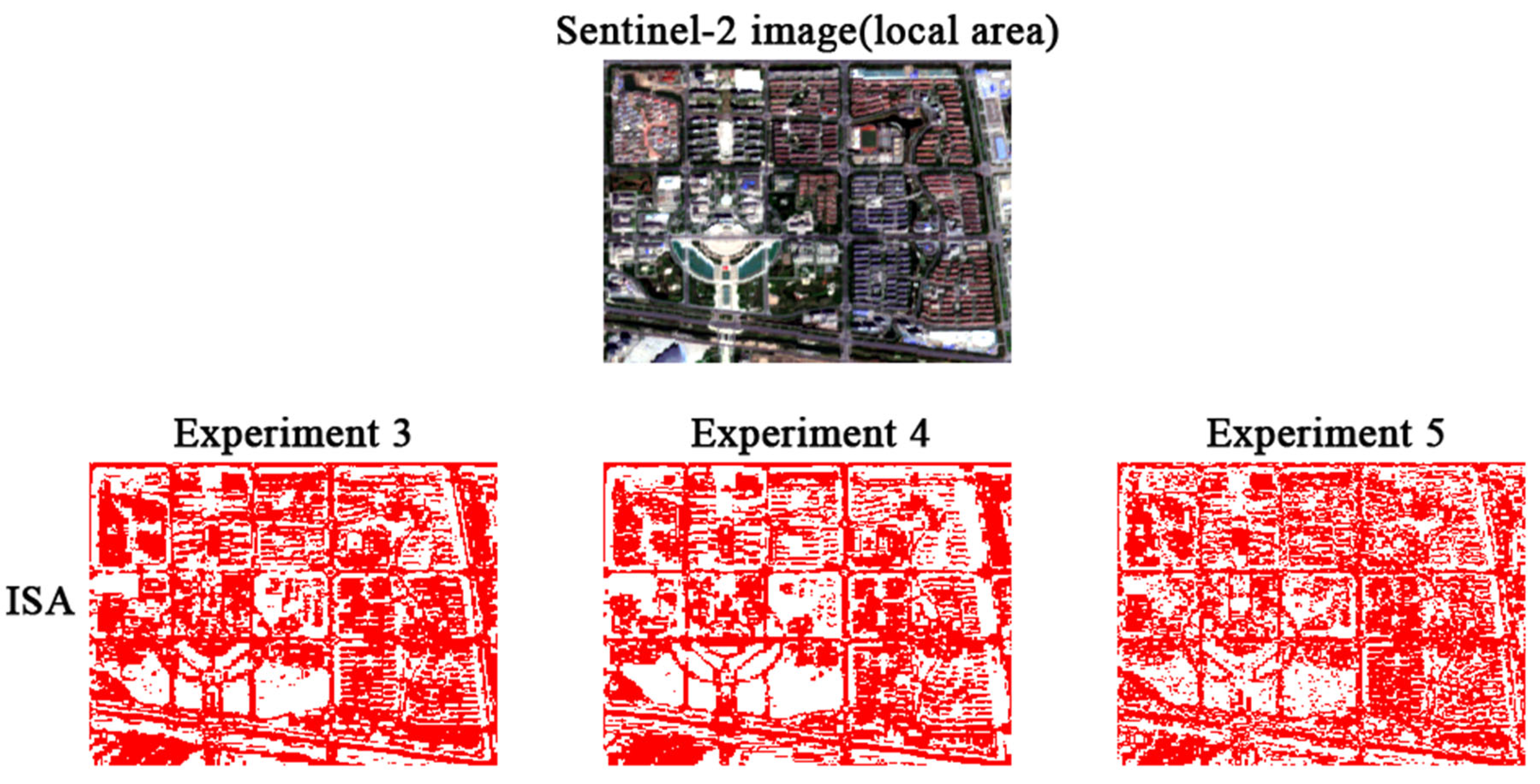
4.1. Comparative Analysis of Different Classification Schemes

In order to verify the influence of RF combined with Sentinel-1/2 data on the accuracy of ISA extraction, several experiments (Table 3) were designed by combining different input features and classifiers. Experiment 1 is a combination of SAR backscattering properties with RF. Experiment 2 aimed to explore the impact of the RF combined with surface reflectance features, spectral indices feature, and textural features on the accuracy of ISA mapping. Experiment 3, 4, 5 only compared the performance of different classifiers (RF, SVM, CART) on the condition of the same input features.
The overall accuracy, kappa coefficient, User ‘s Accuracy and Producer ‘s Accuracy of the above-mentioned five experiments is statistically summarized in Table 4.
From Table 4, it can be observed that the accuracy of Experiment 1 is the lowest (with an overall accuracy of only 59.43% and a kappa coefficient of 0.5492) among all experiments when only backscattering coefficient features were used. According to Table 4, the overall accuracy of Experiment 3 is higher than that of Experiment 2 by about 2.5 percentage points, and the PA and UA of Experiment 3 is higher than that of Experiment 2 by about 5 to 6 percentage points. The inclusion of the backscattering coefficient features further improves the accuracy of ISA extraction. From Figure 6, the ISA is underestimated in both Experiment 1 and 2 while the result of Experiment 3 is in good agreement with the ISA real distribution. Through comprehensive analysis of the above three experiments, although the accuracy of classification only using SAR data is very low, it can be used as an effective supplementary of optical images to improve the quality of classification result.
Figure 7 shows the local region of the entire ISA results generated by three different classification methods for the purpose of comparison. According to Figure 7, the result of the RF visually outperforms the SVM and CART. Compared with the RF, the ISA result yielded by the SVM and CART was underestimated. Meanwhile, the pixels of the ISA based on the SVM and CART are more dispersed. From Table 4, the overall accuracy of the RF is highest compared with that of the SVM and CART, reaching 95.46%. The OA of classification of the SVM ranked the second (90.87%). The OA of classification of the CART is the lowest.
Considering that kappa has limitations in supporting classification accuracy assessment [48,49,50,51], quantity disagreement and allocation disagreement [51] were adopted to further assess the classification accuracy (Table 5).
It can be seen from Table 5 that the RF has the lowest quantity and allocation disagreement among the three methods. This finding further suggests the RF outperforms the other two algorithm in ISA mapping.

4.2. Accuracy and Extraction Results of ISA

In order to explore the spatial–temporal evolution characteristics of ISA in the YRDHEEZ, the annual continuous time-series ISA data from 2018 to 2022 was produced using the proposed method. Table 6 shows the OA and Kappa of annual ISA result map in the YRDHEEZ. A high average OA (94.84%) and Kappa (0.9393) revealed that a series of promising ISA map was obtained, and it further demonstrated the effectiveness and advantage of the designed workflow in this study. Meanwhile, Table 6 also implied that the time-series classification result met the requirements for subsequent ISA evolution analysis.
To yield an annual continuous spatial–temporal distribution map of the ISA, build-up area and rural settlements in classification result image were combined as the ISA while the remaining surface types were integrated into pervious surfaces (Figure 8). Combined with the corresponding true color image and Figure 8, it can be observed that the annual ISA map is consistent with its real ISA distribution. However, the distribution of the ISA exhibited strong spatial heterogeneity. The center of each county in this region holds high density ISA while the area far from it commonly shows low density ISA, which suggests that the increase of the ISA was still strongly dependent on the impetus of the county center in the local area. Due to the short time interval of study period and the vast area of the YRDHEEZ, it is very difficult to identify the remarkable difference only from the annual ISA map in Figure 8.

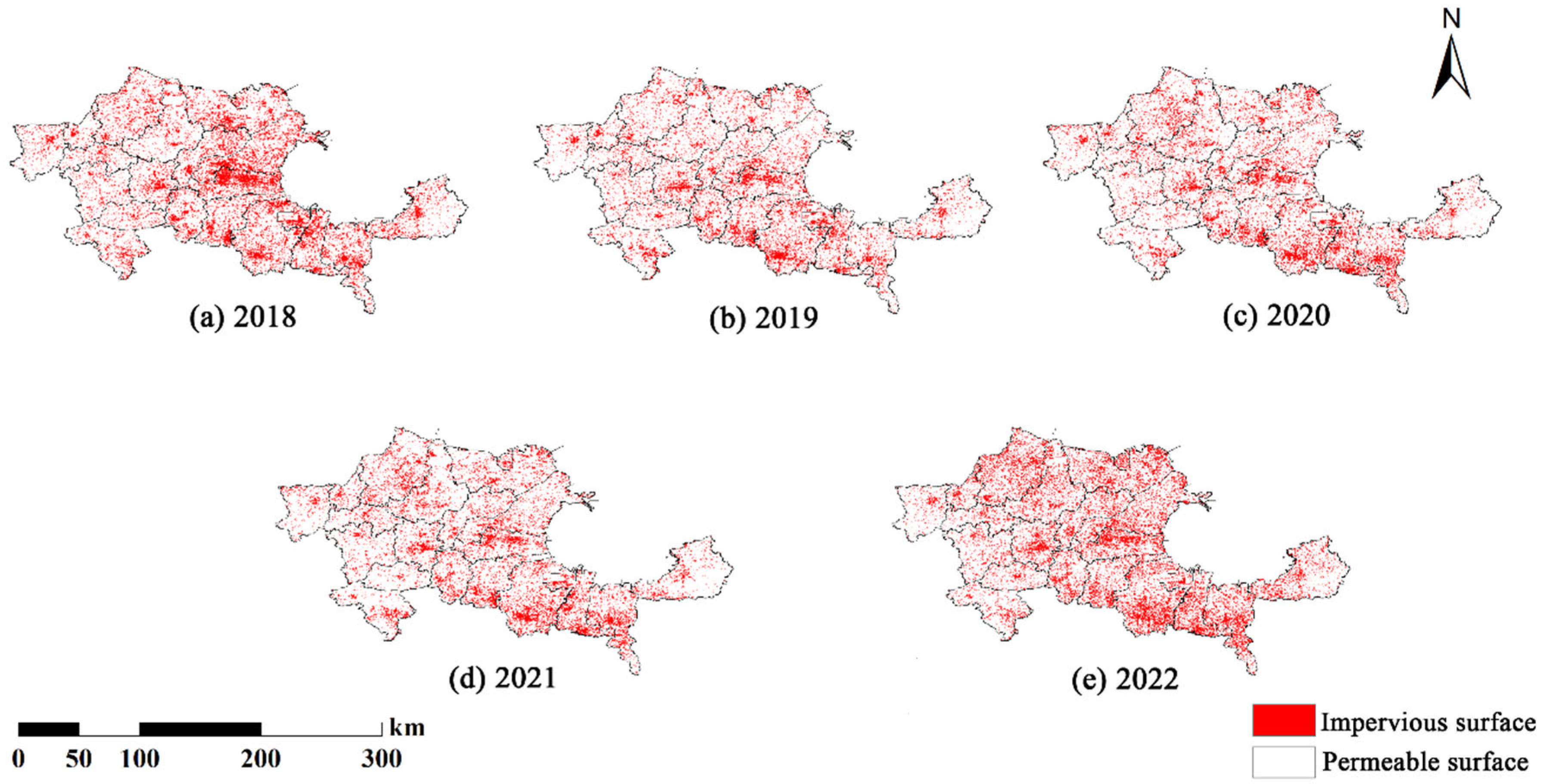
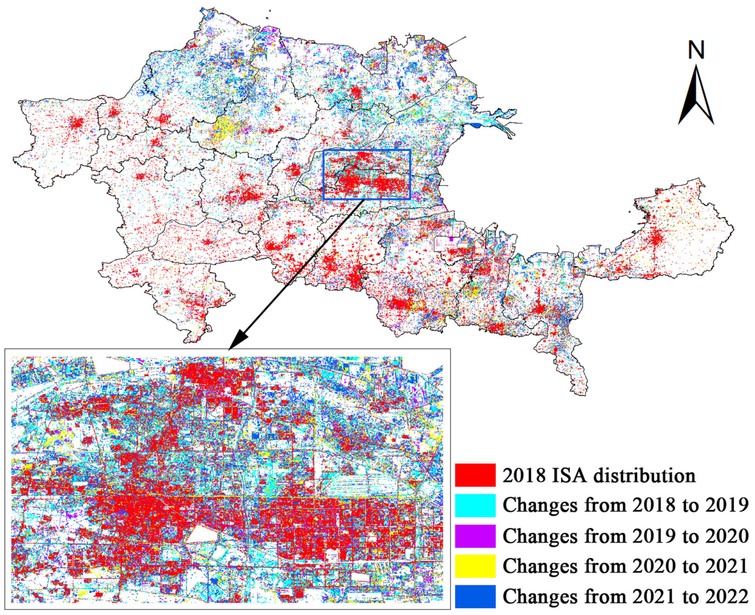
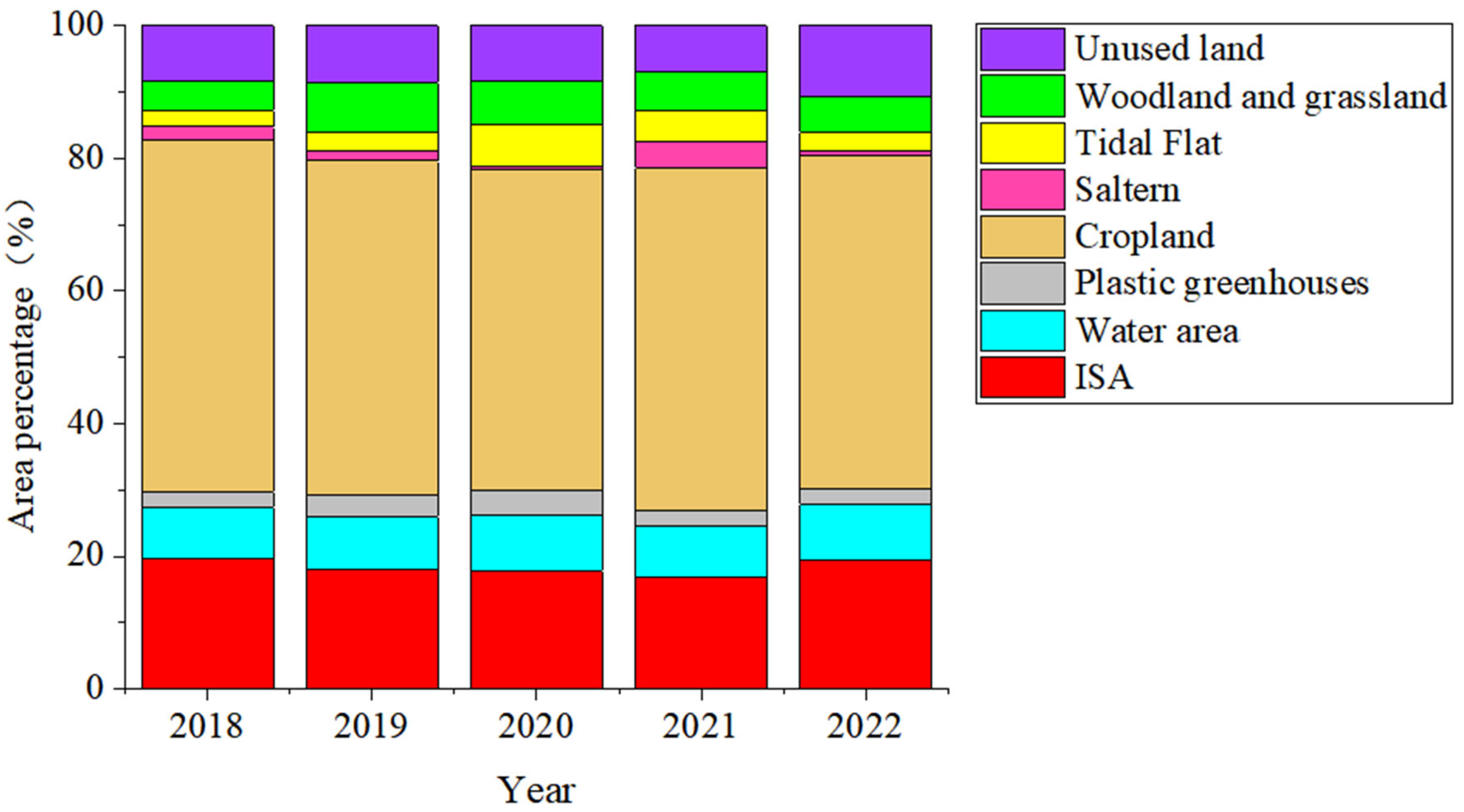
4.3. Spatial–Temporal Evolution Analysis

Based on the annual ISA in the YRDHEEZ for the past 5 years, a spatial–temporal evolution map was produced, as shown in Figure 9. According to the evolution maps, the ISA was mainly distributed along the central and southern parts of the YRDHEEZ in 2018 while the growth trend of the ISA in the northern part became increasingly obvious over time, with its growth rate reaching the largest after 2021. Overall, the areas with good economic development continue to extend and drive the development of surrounding towns, gradually forming an ISA distribution pattern with the center city in local region as the core and dispersing to surrounding towns and satellite cities.
According to the statistics of eight land use/cover types in Table 7, it can be seen that the ISA area in the last five years shows a decrease at first, then an increase as followed, changing from 5211.39 km2 in 2018 to 4461.93 km2 in 2021, and then, it rises to 5147.02 km2 in 2022 with a change rate of −16.09 km2/year. During 2018–2021, the tendency of the ISA and unused land is mutually corresponding, which is due to the fact that cities in the region were rebuilding and optimizing their internal spatial structures. For 2021 to 2022, the accelerated urban development process and the outside radiation of the central city to the surrounding areas led to an increase in the ISA with a significant decrease in the area of tidal flat and saltern. In addition, waterbody and arable land have a similar rate of change. The area of woodland and grassland increases from the initial 1160.53 km2 to 1421.52 km2 with an overall growth rate of 65.25 km2 annually, which is in line with the requirements of China for the ecological sustainability development.
In order to compare the annual changes of land use/land cover types, a stacked bar (Figure 10) was made based on Table 7 for showing the area percentage of different land use/land cover types annually. From Figure 10, the area percentage of the ISA slightly decreases from 2018 to 2021 while a small increase of area percentage of the ISA occurred in 2022, which was related to a change in local government policies. Furthermore, unused land has a similar trend of change to the ISA. The change trend of woodland and grassland is different from that of the ISA, and the area of woodland and grassland gradually decreases from 2019. The change trend of the area of water, cropland, and plastic greenhouses is not obvious. On the whole, there is no great fluctuation for the area percentage of the annual ISA, which may be attributed to the short duration of the study period.

5. Discussion

5.1. Impact of Including Backscattering Features on ISA Mapping

In this section, we discuss the effect of the addition of the backscattering properties to the extraction of the impervious surface area. According to the results of experimental accuracy calculations given in Table 4, the accuracy is very low if only the backscattering features are used while the accuracy is improved by including the features such as the surface reflectance feature, spectral indices feature, and texture feature (Experiment 2). However, according to Experiment 3, when the inclusion of backscattering properties is integrated with multispectral data, a further, greater accuracy improvement was derived in differentiating built-up, unused land, and fallow land. Commonly, optical multispectral images can play a critical role in identifying different land use/land cover types. However, as mentioned in Section 2.1, the unique geographical location adjacent to the Bohai Sea makes the soil of the YRDHEEZ prone to salinization, which leads to massive unused land. Meanwhile, lots of infertile farmland is required to set aside for years to restore land productivity, which results in the expansion of the fallow land. Through a comparison of spectral characteristics among built-up, unused land, and fallow land, the three kinds of land use/land cover types have a similar spectral signature, which adds difficulty in identifying them when single multispectral data was included in the classification. However, when backscattering properties derived from Sentinel-1 are used as supplementary, the built-up area (an ISA component) can be accurately identified due to its larger surface roughness than unused land and fallow land as well as different dielectric properties. This indicated that introducing radar data into ISA mapping can improve the accuracy of the classification result, and simultaneously, the effectiveness of the proposed method can be justified.

5.2. Comparison with Other Methods

In this section, we focus on the advantage of the proposed method proposed over other ISA mapping methods. To verify the degree of influence of different classification methods on the information extraction result, we designed three experiments as shown in Table 3 by only changing different classifiers on the condition of the same input features. As the commonly used machine learning classification algorithms, CART, SVM, and RF classification algorithms have been widely adopted for the information extraction classification task. The experimental results in this study show that the accuracy of all three methods can be promising. The CART runs faster in the test dataset and can produce feasible and effective results for large data sets in a relatively short time; however, the CART classification has too many isolated image elements and is prone to result in an overfit in modelling for ISA mapping. The SVM only use a few support vectors of classification to identify different land use/land cover, which helps to catch important samples and eliminate a large number of redundant samples and also enable the method to have a better robustness. However, the SVM requires more complicated parameters to be set, which is time-consuming. Regarding the RF, compared with the two methods, less parameters need to be set, and thus, the RF is able to run effectively on large data sets; meanwhile, it introduces randomness, which is less likely to lead to an overfit in the process of modelling. It indicated that the RF algorithm is more advantageous in ISA mapping based on remote sensing images. Moreover, RF can effectively use the differences between samples and select the optimal variables for classification to achieve more accurate classification. In summary, the proposed method has the highest classification accuracy and can achieve accurate ISA extraction.

5.3. The Reason for the Change of the ISA

In this section, we will discuss the factors that leads to the variation of the ISA. The area statistics of the main land use/cover types are shown in Table 7, and it can be observed that the area of the ISA again rebounded after a certain degree of decline from the entire study period. More specifically, in the 2018–2019 interval, the ISA decreases significantly, accompanied by the slight increase of the area of waterbody and tidal flat together with the significant increase of woodland and grassland. The reason for the change is closely related to a series of ecological protection and restoration policies promulgated by the state in order to reduce soil erosion and implement the principle of ecologically sustainable development. In the following 2020 and 2021 year, the ISA continues to decrease at a slow rate, which corresponded to the trend of changing unused land along with the internal spatial restructuring and optimization of the related cities. From 2021 to 2022, the area of the tidal flat and saltern decreases significantly, and the ISA grows. This change trend is closely related to the economic development and the accelerated urban development process, which makes some permeable natural surfaces continuously occupied by impermeable artificial surfaces.

6. Conclusions

Based on the multi-source and multi-modal Sentinel-1/2 remotely sensed data provided by Google Earth Engine (GEE) cloud computing platform, this study developed a novel approach for large-scale ISA mapping in the YRDHEEZ through a combination of random forest algorithm and numerous representative features extracted from Sentinel-1/2, including surface reflectance features, spectral indices feature, GLCM texture features and backscattering properties. Subsequently, the spatial-temporal evolution of ISA in the YRDHEEZ was conducted using an annual time-series of the ISA data from 2018 to 2022. The following conclusions are drawn.
(a) The overall accuracy of ISA mapping ranges from 94.11% to 95.46% for 2018–2022, with an average overall accuracy of 94.84%. Meanwhile, the Kappa coefficient ranges from 0.9345 to 0.9412, with an average Kappa coefficient reaching 0.9393. It shows that the proposed method in this study can achieve a relatively better ISA extraction result.
(b) For the seaside area prone to salinization and secondary salinization like the YRDHEEZ, integrating backscattering properties with multi-spectral data can make a great accuracy improvement in differentiating built-up, unused land, and fallow land, which demonstrated that multisource and multimodal data can play a positive role in generating accurate large-scale ISA data.
(c) In the past five years, the area of the ISA in the YRDHEEZ has decreased from 5211.39 km2 in 2018 to 5147.02 km2 in 2022, with an average change rate of-16.09 km2 / year, which implied that a series of development plans introduced by the state have played a positive effect. Spatial pattern analysis revealed that the ISA increased rapidly in the central and southern parts of the YRDHEEZ during the study period. The distribution of the ISA exhibited strong spatial heterogeneity. The center of each county in this region holds high density ISA while the area far from it commonly shows low density ISA, which suggested that the increase of ISA was still strongly dependent on the impetus of the county center in the local area. Overall, the areas with good economic development continue to extend and drive the development of surrounding towns, gradually forming the current ISA pattern with the center city in the local region as the core and dispersing to surrounding towns and satellite cities.
The research we performed mainly focused on the implementation of the large-scale ISA mapping as well as the evolution analysis of the ISA in the YRDHEEZ. However, limited by the launch time of the Sentinel-1/2 satellite, only a relatively shorter period ranging from 2018 to 2022 was considered, and a few factors were adopted in the ISA evolution analysis of the YRDHEEZ. In the future, we will take more factors into account in the ISA evolution analysis of this region.

Author Contributions

Methodology, J.L.; software, J.L.; validation, Y.L.; formal analysis, J.L. and Y.L.; data curation, Y.L.; writing—original draft preparation, J.L. and Y.L.; writing—review and editing, J.L., Y.L., Y.Z. and X.L. All authors have read and agreed to the published version of the manuscript.

Funding

This research was funded by the National Natural Science Foundation of China, grant number 42171113, 42271112 and Shandong Natural Science Foundation, grant number ZR2020QD017, ZR2020QD049.

Acknowledgments

The authors thank Google Earth Engine for providing computer resources and Sentinel-1/2 Data.

Conflicts of Interest

The authors declare no conflict of interest.

References

  1. Arnold, C.L.; Gibbons, C.J. Impervious surfaces Coverage: The Emergence of a Key Environmental Indicator. J. Am. Plan. Assoc. 1996, 62, 243–258. [Google Scholar] [CrossRef]
  2. Yuan, F.; Bauer, M.E. Comparison of Impervious surfaces area and normalized difference vegetation index as indicators of surface urban heat island effects in Landsat imagery. Remote Sens. Environ. 2006, 106, 375–386. [Google Scholar] [CrossRef]
  3. Jia, Y.; Tang, L.; Wang, L. Influence of Ecological Factors on Estimation of Impervious surfaces Area Using Landsat 8 Imagery. Remote Sens. 2017, 9, 751. [Google Scholar] [CrossRef] [Green Version]
  4. Yao, Z.; Meng, Q.; Sun, Z.; Liu, S.; Zhang, L. Temporal and spatial correlation between Impervious surfaces and surface runoff: A case study of the main urban area of Hangzhou city. J. Remote Sens. 2020, 24, 182–198. [Google Scholar]
  5. Schueler, T. The Importance of Imperviousness. Watershed Prot. Tech. 1994, 1, 100–111. [Google Scholar]
  6. Song, X.P.; Sexton, J.O.; Huang, C.Q.; Channan, S.; Townshend, J.R. Characterizing the magnitude, timing and duration of urban growth from time series of Landsat-based estimates of impervious cover. Remote Sens. Environ. 2016, 175, 1–13. [Google Scholar] [CrossRef]
  7. Dou, Y.Y.; Kuang, W.H. A comparative analysis of urban Impervious surfaces and green space and their dynamics among 318 different size cities in China in the past 25 years. Sci. Total Environ. 2020, 706, 135828. [Google Scholar] [CrossRef]
  8. Wu, C.; Murray, A.T. Estimating Impervious surfaces distribution by spectral mixture analysis. Remote Sens. Environ. 2003, 84, 493–505. [Google Scholar] [CrossRef]
  9. Lu, D.S.; Li, G.Y.; Kuang, W.H.; Moran. Methods to extract Impervious surfaces areas from satellite images. Int. J. Digit. Earth 2014, 7, 93–112. [Google Scholar] [CrossRef]
  10. Piyoosh, A.K.; Ghosh, S.K. Development of a modified bare soil and urban index for Landsat 8 satellite data. Geocarto Int. 2018, 33, 423–442. [Google Scholar] [CrossRef]
  11. Shrestha, B.; Ahmad, S.; Stephen, H. Fusion of Sentinel-1 and Sentinel-2 data in mapping the Impervious surfaces at city scale. Environ. Monit. Assess. 2021, 193, 556. [Google Scholar] [CrossRef] [PubMed]
  12. Liu, J.; Liu, C.; Feng, Q.; Ma, Y. Subpixel Impervious surfaces estimation in the Nansi Lake Basin using random forest regression combined with GF-5 hyperspectral data. J. Appl. Remote Sens. 2020, 14, 34515. [Google Scholar] [CrossRef]
  13. Liu, S.; Li, Q. Composite kernel support vector regression model for hyperspectral image Impervious surfaces extraction. J. Remote Sens. 2016, 20, 420–430. [Google Scholar]
  14. Zhang, L.; Weng, Q. Annual dynamics of Impervious surfaces in the Pearl River Delta, China, from 1988 to 2013, using time series Landsat imagery. ISPRS J. Photogramm. Remote Sens. 2016, 113, 86–96. [Google Scholar] [CrossRef]
  15. Liu, C.; Feng, Q.; Jin, D.; Shi, T.; Liu, J.; Zhu, M. Application of random forest and Sentinel-1/2 in the information extraction of impervious layers in Dongying City. Remote Sens. Nat. Resour. 2021, 33, 253–261. [Google Scholar]
  16. Zhai, K.; Wu, X.; Qin, Y.; Yu, L.; Du, P. Extraction and spatial analysis of Impervious surfaces in the Bohai Bay region based on OLI imagery. Resour. Sci. 2015, 37, 1920–1928. [Google Scholar]
  17. Duan, F.; Zhang, F.; Liu, C. Extraction of the Impervious surfaces of typical cities in Xinjiang based on Sentinel-2A/B and spatial difference analysis. J. Remote Sens. 2022, 26, 1469–1482. [Google Scholar]
  18. Piyoosh, A.K.; Ghosh, S.K. Semi-automatic mapping of anthropogenic Impervious surfaces in an urban/suburban area using Landsat 8 satellite data. GIsci. Remote Sens. 2017, 54, 471–494. [Google Scholar] [CrossRef]
  19. Li, S.; Li, S.; Kang, X. Development status and future prospects of multi-source remote sensing image fusion. J. Remote Sens. 2021, 25, 148–166. [Google Scholar]
  20. Mandianpari, M.; Salehi, B.; Mohammadimanesh, F.; Motagh, M. Random forest wetland classification using ALOS-2 L-band, RADARSAT-2 C-band, and TerraSAR-X imagery. ISPRS J. Photogramm. Remote Sens. 2017, 130, 13–31. [Google Scholar] [CrossRef]
  21. Sun, G.; Cheng, J.; Zhang, A.; Jia, X.; Yao, Y.; Jiao, Z. Hierarchical fusion of optical and dual-polarized SAR on Impervious surfaces mapping at city scale. ISPRS J. Photogramm. Remote Sens. 2022, 184, 264–278. [Google Scholar] [CrossRef]
  22. Li, F.; Li, E.; Saibati, A.; Zhang, L.; Liu, W.; Hu, J. Estimation of large-scale Impervious surfaces percentage by fusion of multi-source time series remote sensing data. J. Remote Sens. 2020, 24, 1243. [Google Scholar] [CrossRef] [Green Version]
  23. Chen, X.; Yang, K.; Wang, J.; Wang, Z.; Wang, L.; Su, F. Improving long-term Impervious surfaces percentage mapping in mountainous areas based on multi-source remote sensing data. Geocarto Int. 2022, 1–23. [Google Scholar] [CrossRef]
  24. Zhang, X.; Liu, L.; Wu, C.; Chen, X.; Gao, Y.; Xie, S.; Zhang, B. Development of a global 30 m Impervious surfaces map using multisource and multitemporal remote sensing datasets with the Google Earth Engine platform. Earth Syst. Sci Data. 2020, 12, 1625–1648. [Google Scholar] [CrossRef]
  25. Jiang, L.; Liao, M.; Lin, H.; Yang, L.; Wang, C. Estimating Urban Impervious surfaces Percentage with ERS-1/2 InSAR Data. J. Remote Sens. 2008, 12, 176–185. [Google Scholar]
  26. Zhang, H.; Lin, H.; Wang, Y. A new scheme for urban Impervious surfaces classification from SAR images. ISPRS J. Photogramm. Remote Sens. 2018, 139, 103–118. [Google Scholar] [CrossRef]
  27. Lin, Y.; Zang, H.; Lin, H.; Paolo, E.G.; Liu, X. Incorporating synthetic aperture radar and optical images to investigate the annual dynamics of anthropogenic Impervious surfaces at large scale. Remote Sens. Environ. 2020, 242, 111757. [Google Scholar] [CrossRef]
  28. Zhang, H.; Lin, H.; Li, Y.; Zang, Y.; Fang, C. Mapping urban Impervious surfaces with dual-polarimetric SAR data: An improved method. Landsc. Urban Plan. 2016, 151, 55–63. [Google Scholar] [CrossRef]
  29. Wang, X.; Tian, J.; Li, X.; Wang, L.; Gong, H.; Chen, B.; Li, X.; Guo, J. Benefits of Google Earth Engine in remote sensing. J. Remote Sens. 2022, 26, 299. [Google Scholar] [CrossRef]
  30. Tamiminia, H.; Salehi, B.; Mahdianpari, M.; Quackenbush, L.; Adeli, S.; Brisco, B. Google Earth Engine for geo-big data applications: A meta-analysis and systematic review. ISPRS J. Photogramm. Remote Sens. 2020, 164, 152–170. [Google Scholar] [CrossRef]
  31. Wang, L.; Diao, C.; George, X.; Yin, D.; Lu, Y.; Zou, S.; Tyler, A.E. A summary of the special issue on remote sensing of land change science with Google earth engine. Remote Sens. Environ. 2020, 248, 112002. [Google Scholar] [CrossRef]
  32. Gorelick, N.; Hancher, M.; Dixon, M.; Ilyushchenko, S.; Thau, D.; Moore, R. Google Earth Engine: Planetary-scale geospatial analysis for everyone. Remote Sens. Environ. 2017, 202, 18–27. [Google Scholar] [CrossRef]
  33. Xu, H.; Wei, Y.; Liu, C.; Li, X.; Fang, H. A Scheme for the Long-Term Monitoring of Impervious−Relevant Land Disturbances Using High Frequency Landsat Archives and the Google Earth Engine. Remote Sens. 2019, 11, 1891. [Google Scholar] [CrossRef] [Green Version]
  34. Lu, X.; Huang, Y.; Hong, J.; Zeng, D.; Yang, L. Spatial and temporal variations in wetland landscape patterns in the Yellow River Delta based on Landsat images. China Environ. Sci. 2018, 38, 4314–4324. [Google Scholar]
  35. Perni, A.; Martinez-Paz, J.M. Measuring conflicts in the management of anthropized ecosystems: Evidence from a choice experiment in a human-created Mediterranean wetland. J. Environ. Manag. 2017, 203, 40–50. [Google Scholar] [CrossRef]
  36. Yue, J.; Zhao, S.; Cheng, H.; Duan, X.; Shi, H.; Wang, L.; Duan, Z. Distribution of Micro-plastics in the Soil Covered by Different Vegetation in Yellow River Delta Wetland. Environ. Sci. 2021, 42, 204–210. [Google Scholar]
  37. Zhang, S.; Dong, H.; Zeng, W. The time-space evolution characteristics of the vulnerability of land ecosystems and influencing factors: A case study of the Yellow River Delta Efficiency Eco-economic Zone. China Environ. Sci. 2019, 39, 1696–1704. [Google Scholar]
  38. Shao, Z.; Fu, H.; Fu, P.; Yin, L. Mapping Urban Impervious surfaces by Fusing Optical and SAR Data at the Decision Level. Remote Sens. 2016, 8, 945. [Google Scholar] [CrossRef] [Green Version]
  39. Feng, X.; Shao, Z.; Huang, X.; He, L.; Lv, X.; Zhuang, Q. Integrating Zhuhai-1 Hyperspectral Imagery With Sentinel-2 Multispectral Imagery to Improve High-Resolution Impervious surfaces Area Mapping. IEEE J. Sel. Top. Appl. Earth Obs. Remote Sens. 2022, 15, 2410–2424. [Google Scholar] [CrossRef]
  40. Kaufman, Y.J.; Tanre, D. Atmospherically resistant vegetation index (ARVI) for EOS-MODIS. IEE Trans. Geosci. Remote Sens. 1992, 30, 261–270. [Google Scholar] [CrossRef]
  41. Xu, H. A Study on Information Extraction of Water Body with the Modified Normalized Difference Water Index (MNDWI). J. Remote Sens. 2005, 5, 589–595. [Google Scholar]
  42. Cha, Y.; Ni, S.; Yang, S. An Effective Approach to Automatically Extract Urban Land-use from TM imagery. J. Remote Sens. 2003, 1, 37–40. [Google Scholar]
  43. Dong, X.; Meng, Z.; Wang, Y.; Zhang, Y.; Sun, H.; Wang, Q. Monitoring Spatiotemporal Changes of Impervious surfaces in Beijing City Using Random Forest Algorithm and Textural Features. Remote Sens. 2021, 13, 153. [Google Scholar] [CrossRef]
  44. Bramhe, V.S.; Ghosh, S.K.; Garg, P.K. Extraction of built-up areas from Landsat-8 OLI data based on spectral-textural information and feature selection using support vector machine method. Geocarto Int. 2020, 35, 1067–1087. [Google Scholar] [CrossRef]
  45. Szantoi, Z.; Escobedo, F.; Abd-Elrahman, A.; Smith, S.; Pearlstine, L. Analyzing fine-scale wetland composition using high resolution imagery and texture features. Int. J. Appl. Earth Obs. Geoinf. 2013, 23, 204–212. [Google Scholar] [CrossRef]
  46. Breiman, L. Random Forests. Mach. Learn. 2001, 45, 5–32. [Google Scholar] [CrossRef] [Green Version]
  47. Wu, L.; Li, X.; Mao, D.; Wang, Z. Urban land use classification based on remote sensing and multi-source geographic data. Remote Sens. Nat. Resour. 2022, 34, 127–134. [Google Scholar]
  48. Pontius, R.G., Jr.; Millones, M. Death to Kappa: Birth of quantity disagreement and allocation disagreement for accuracy assessment. Int. J. Remote Sens. 2011, 32, 4407–4429. [Google Scholar] [CrossRef]
  49. Olofsson, P.; Foody, G.M.; Herold, M.; Stehman, S.V.; Woodcock, C.E.; Wulder, M.A. Good practices for estimating area and assessing accuracy of land change. Remote Sens. Environ. 2014, 148, 42–57. [Google Scholar] [CrossRef]
  50. Stehman, S.V.; Foody, G.M. Key issues in rigorous accuracy assessment of land cover products. Remote Sens. Environ. 2019, 231, 111199. [Google Scholar] [CrossRef]
  51. Foody, G.M. Explaining the unsuitability of the kappa coefficient in the assessment and comparison of the accuracy of thematic maps obtained by image classification. Remote Sens. Environ. 2020, 239, 111630. [Google Scholar] [CrossRef]
Figure 1. False color composite of the study area: Band8 (nir), Band4 (red) and Band3 (green) of Sentinel-2 MSI.
Remotesensing 15 00136 g001
Figure 2. Methodology flowchart.
Remotesensing 15 00136 g002
Figure 3. Flow of extraction of backscattering coefficient characteristics.
Remotesensing 15 00136 g003
Figure 4. Sample selection area.
Remotesensing 15 00136 g004
Figure 5. Schematic diagram of Random Forest for classification.
Remotesensing 15 00136 g005
Figure 6. ISA Classification results for different feature sets.
Remotesensing 15 00136 g006
Figure 7. ISA classification results for different classifiers.
Remotesensing 15 00136 g007
Figure 8. Spatial-temporal distribution of ISA over the last 5 years.
Remotesensing 15 00136 g008
Figure 9. Spatial-temporal evolution of ISA in the last 5 years.
Remotesensing 15 00136 g009
Figure 10. Annual area comparison of different LULC types.
Remotesensing 15 00136 g010
Table 1. Multi-source image data.
Image SourceImage TypeImage SelectionGet the DateResolution
Sentinel-1 SARRadar imagesSynthetic Aperture Radar;
Level-1 ground-range Multiview images in IW imaging mode;
Dual-polarization mode (VV + VH);
Revisit cycle of 5 days
2018 to 2022
(April, May, and June each year)
10 m
Sentinel-2 MSIOptical imagesMultispectral images;
Bands: B2, B3, B4, B5, B6, B7, B8, B8A, B11, B12;
Revisit cycle of 5 days
2018 to 2022
(April, May, and June each year)
10 m + 20 m
Table 2. Classification samples.
Land CoverTraining Sample/pcTest Sample/pcClassification Criteria
Built-up350150Urban buildings, car parks, concrete roads, etc.
Rural Settlement350150Gathering places belonging to the commune
Water area350150Lakes, rivers reservoirs, etc.
Plastic greenhouses350150Arable land covered with plastic film for growing crops
Fallow land350150cropland temporarily not planted with crops
Arable land350150Arable land planted with crops
Saltern350150Coastal evaporative salt production site
Tidal Flat350150High and low tide junction areas at water boundaries
Woodland and grassland350150Forest, grassland, shrub, and other vegetated land
Unused land350150Sites under construction or bare land
Table 3. Validation experiment.
Experiment NumberInput FeaturesClassifiers
Experiment 1multi-polarization (VV and VH backscattering coefficients)RF
Experiment 2Surface reflectance features + spectral features + texture featuresRF
Experiment 3Surface reflectance features + spectral features + textural features + multi-polarization (VV and VH backscattering coefficients)RF
Experiment 4Surface reflectance features + spectral features + textural features + multi-polarization (VV and VH backscattering coefficients)SVM
Experiment 5Surface reflectance features + spectral features + textural features + multi-polarization (VV and VH backscattering coefficients)CART
Table 4. Accuracy comparison with different experiments.
TypeExperiment 1Experiment 2Experiment 3Experiment 4Experiment 5
PAUAPAUAPAUAPAUAPAUA
Built-up45.99 59.43 85.26 93.01 90.79 97.87 71.01 94.23 78.91 84.87
Rural Settlement51.33 51.68 84.62 87.30 90.65 90.65 95.77 80.00 77.18 85.82
Water area72.60 55.79 100.00 100.00 100.00 98.67 100.00 98.28 98.59 99.29
Plastic greenhouses70.55 61.31 98.03 96.75 99.33 99.33 98.08 98.08 95.80 95.80
Fallow land60.00 52.33 80.99 87.12 85.71 85.04 65.10 75.78 73.10 67.09
arable land90.00 84.56 98.78 99.39 99.35 98.71 100.00 95.71 96.45 96.45
Saltern52.98 57.14 98.57 99.28 98.55 100.00 97.95 100.00 100.00 96.24
Tidal Flat47.62 58.82 99.28 95.83 100.00 96.55 95.48 93.08 94.44 95.63
Woodland and grassland71.52 66.86 99.32 95.45 100.00 96.40 100.00 96.71 97.30 92.90
Unused land33.96 44.26 91.53 80.60 88.41 89.05 80.00 73.28 79.41 78.26
OA (%)59.4393.8295.4690.8789.17
Kappa 0.54920.93130.94950.89850.8796
Note. PA, %; UA, %.
Table 5. Comparison of quantity and allocation disagreement among three methods.
MethodQuantity Disagreement (%)Allocation Disagreement (%)
RF0.913.63
SVM3.925.20
CART1.908.93
Table 6. Overall accuracy and kappa coefficient for time-series ISA.
Date/Year20182019202020212022
OA (%)94.1195.1795.4694.8894.59
Kappa0.93450.94090.94010.94120.9399
Table 7. Area statistics of different land use/cover types.
Area/km2ISAWater AreaPlastic GreenhousesCroplandSalternTidal FlatWoodland and GrasslandUnused Land
20185211.39 2062.98 619.44 14,045.82 518.31 669.30 1160.53 2212.24
20194790.67 2107.57 859.01 13,338.10 400.32 729.96 2019.76 2254.61
20204734.02 2195.12 994.01 12,829.27 101.75 1698.36 1742.64 2204.85
20214461.93 2064.86 607.74 13,702.88 1018.07 1234.30 1564.41 1845.80
20225147.02 2248.28 576.56 13,323.31 194.46 772.39 1421.52 2816.46
Disclaimer/Publisher’s Note: The statements, opinions and data contained in all publications are solely those of the individual author(s) and contributor(s) and not of MDPI and/or the editor(s). MDPI and/or the editor(s) disclaim responsibility for any injury to people or property resulting from any ideas, methods, instructions or products referred to in the content.

