Multisite and Multitemporal Grassland Yield Estimation Using UAV-Borne Hyperspectral Data

Abstract

Grassland ecosystems can be hotspots of biodiversity and act as carbon sinks while at the same time providing the basis of forage production for ruminants in dairy and meat production. Annual grassland dry matter yield (DMY) is one of the most important agronomic parameters reflecting differences in usage intensity such as number of harvests and fertilization. Current methods for grassland DMY estimation are labor-intensive and prone to error due to small sample size. With the advent of unmanned aerial vehicles (UAVs) and miniaturized hyperspectral sensors, a novel tool for remote sensing of grassland with high spatial, temporal and radiometric resolution and coverage is available. The present study aimed at developing a robust model capable of estimating grassland biomass across a gradient of usage intensity throughout one growing season. Therefore, UAV-borne hyperspectral data from eight grassland sites in North Hesse, Germany, originating from different harvests, were utilized for the modeling of fresh matter yield (FMY) and DMY. Four machine learning (ML) algorithms were compared for their modeling performance. Among them, the rule-based ML method Cubist regression (CBR) performed best, delivering high prediction accuracies for both FMY (nRMSE_p 7.6%, $R_p^2$ 0.87) and DMY (nRMSE_p 12.9%, $R_p^2$ 0.75). The model showed a high robustness across sites and harvest dates. The best models were employed to produce maps for FMY and DMY, enabling the detailed analysis of spatial patterns. Although the complexity of the approach still restricts its practical application in agricultural management, the current study proved that biomass of grassland sites being subject to different management intensities can be modeled from UAV-borne hyperspectral data at high spatial resolution with high prediction accuracies.

1. Introduction

The importance of grassland is manifold and comprises ecosystem services such as carbon storage as well as agronomic values such as fodder for milk and meat production [1]. Simultaneously, the global area of grasslands is shrinking continuously, which is strongly linked to a loss of biodiversity. Grassland management can be classified based on the intensity (e.g., application of fertilizer, number of harvests). While extensive grassland management in Central Europe can be found on marginal lands in the absence of fertilization, intensive grassland management includes high inputs of fertilizers such as manure. These different management strategies lead to a different number of harvests and harvest dates. While extensive grasslands are harvested one to three times a year with a focus on nature conservation (e.g., habitat for rare species, invasive species management), intensively managed grasslands are harvested up to six times per year with a strong focus on yield maximization [2].

Forage yield is traditionally estimated using labor-intensive clipping of sampling areas within the field or using canopy height [3] or density measurements [4]. However, spatial continuity of the sampling and a reliable yield estimation along a whole growing period is almost impossible to achieve. For more than a decade, remote-sensing-based approaches have been tested for overcoming these limitations [5]. While some studies used mobile robotic vehicles for collecting spectral information with the aim of biomass estimation [6] on a limited number of grassland sites, others such as [7] utilized satellites collecting spectral information with a reduced spatial resolution but at a more extensive spatial coverage. While the first approach offers the advantage of high spatial resolution, although constrained by limited spatial coverage, the second method’s abilities to analyze within-field forage yield variability are restricted by low spatial resolution. Recent technical developments made it possible that unmanned aerial vehicles (UAVs) equipped with different sensors such as true color cameras [8], multispectral cameras [9] or hyperspectral cameras [10] can be used for forage yield estimation. A frequent limitation of the studies using UAVs is the low number of sampling intervals or limited representativeness as only a low number of sites and management intensities can be assessed [11,12,13].

Various statistical approaches have been evaluated to exploit the full potential of spectral information to gain the optimal yield prediction accuracy. While some studies used spectral indices (i.e., a combination of two or more spectral bands in simple mathematical combinations) coupled with linear regression approaches [14,15], various machine learning (ML) methods were applied for hyperspectral data analysis [9,16]. However, no single ML method so far has proven superior and always performed best. Thus, an evaluation of several ML methods is recommended [17].

Another difficulty with hyperspectral data is the redundancy of information among the numerous bands. To reduce redundancy, feature selection has been shown to reduce model complexity without degrading (and sometimes increasing) model accuracies [18]. There are several methods available for feature selection, such as VSURF [19] and Boruta [20].

The objectives of this study were the development and evaluation of UAV-based models with the goal of forage yield estimation of eight grassland habitats along a gradient of management intensities. The management intensity was categorized based on the amount of fertilizer application as well as the number of harvests and the harvest dates. The models should be stable among the habitats and throughout the phenological phases of the grasslands. Therefore, several ML methods were tested and evaluated.

Specific aims were as follows:

• Identification of the optimal ML approach for forage yield estimation of grassland habitats characterized by different management intensities.
• Evaluation of prediction performance stability of the ML approach throughout the growing season and between different geographic regions.

2. Materials and Methods

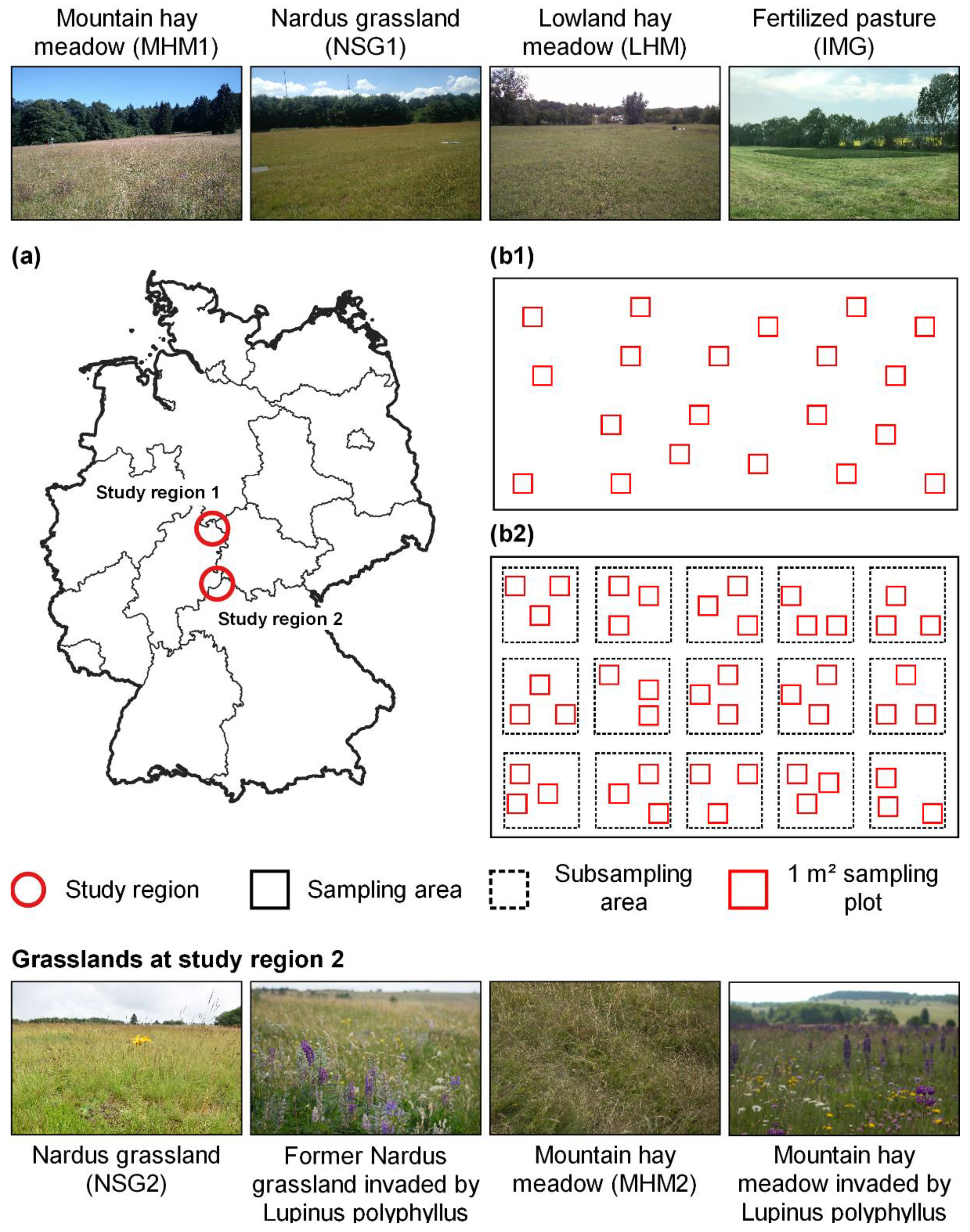
2.1. Study Sites

Data acquisition took place in the vegetation period between May and July 2018 at eight grassland sites differing in grassland composition and management intensity. Four sites were located around Witzenhausen, Werra-Meißner District, North Hesse, Germany, at a height between 136 to 718 m above mean sea level (MSL), while another four sites were located at the Rhön Biosphere Reserve near Fulda (Hesse, Germany) at heights between 794 and 887 m MSL (Figure 1,

Table 1. Overview of examined grassland sites. The number of cuts and number of sampling campaigns differ, as at the sites in Rhön Biosphere Reserve, undisturbed grassland swards were harvested at multiple dates, while at the sites in Werra-Meißner-District, the same grassland sward received multiple cuts.

Sampling Region	Grassland Site	Vegetation Type (Plant Community)	Elevation (m MSL), Coordinates	Intensity of Use	Number of Cuts/Sampling Campaigns/Sampling Plots
Werra-Meißner district	MHM1	Mountain hay meadow (Geranio-Trisetetum)	684, 51°12′48.3″N 9°50′31.5″E	Nature conservation grassland, late harvest, no fertilization	1/1/20
	NSG1	Soil-moist Nardus grassland (Juncetum squarrosi)	718, 51°12′49.4″N 9°50′57.3″E		1/1/20
	LHM	Lowland hay meadow (Arrhenatheretum elatioris)	135, 51°20′59.0″N 9°52′16.5″E	Extensive alluvial grassland, no fertilization	2/2/20
	IMG	Fertilized pasture (Lolio-Cynosuretum)	199, 51°23′32.9″N 9°55′51.2″E	Intensive grassland, fertilized	3/3/20
Rhön Biosphere Reserve	NSG2	Periodically wet Nardus grassland (Polygalo-Nardetum)	822, 50°28′44.0″N 9°58′17.1″E	Nature conservation grassland, late harvest, no fertilization	1/3/15
	NSGL	Former Nardus grassland invaded by Lupinus polyphyllus (Polygalo-Nardetum)	846, 50°29′17.1″N 10°03′40.9″E		1/3/15
	MHM2	Mountain hay meadow (Geranio-Trisetetum)	739, 50°28′58.4″N 9°59′09.9″E		1/3/15
	MHML	Mountain hay meadow invaded by Lupinus polyphyllus (Geranio-Trisetetum)	839, 50°28′45.0″N 10°02′34.6″E		1/3/15

). Central Europe faced a severe drought during 2018, with precipitation in Hesse from February to November at only 54% (356 mm) of the long-term average (661 mm) [21].

For the present study, data from two study regions in Central Germany, namely Werra-Meißner District (EPSG 4326: 9.9°N, 51.3°E) and Rhön Biosphere Reserve (EPSG 4326: 10.0°N, 50.5°E), were combined (Figure 1). Although the sampling design was slightly different, the datasets from both regions could still be combined, as the sampling plot size, the remote sensing data collection and the biomass sample treatment were similar. The study sites near Witzenhausen, Werra-Meißner District, received one (MHM1, NSG1), two (LHM) and three cuts (IMG) in 2018 (Figure 2). At each study site in Werra-Meißner District, a rectangular sampling area of 25 × 50 m (1250 m²) was established, and 20 randomly distributed 1 m² sampling plots were placed (Figure 1(b1)). For the sites in the Rhön Biosphere Reserve, a 50 × 30 m (1500 m²) sampling area was established at all four grasslands. Within each site, 15 subsampling areas (64 m²) were placed within an equally spaced grid. In each subsampling area, three randomly distributed 1 m² sampling plots were placed (Figure 1(b2)). For biomass sampling at Rhön Biosphere Reserve, three cutting dates were selected, representing the regular harvest date according to nature conservation rules (15 June), an antedated harvest optimal for removing the invasive plant species Lupinus polyphyllus (1 June) and a late harvest date that is common in the region, when the weather does not allow earlier harvest (1 July). Biomass was harvested within the 1 m² sampling plots of five subsampling areas per grassland site during every sampling date.

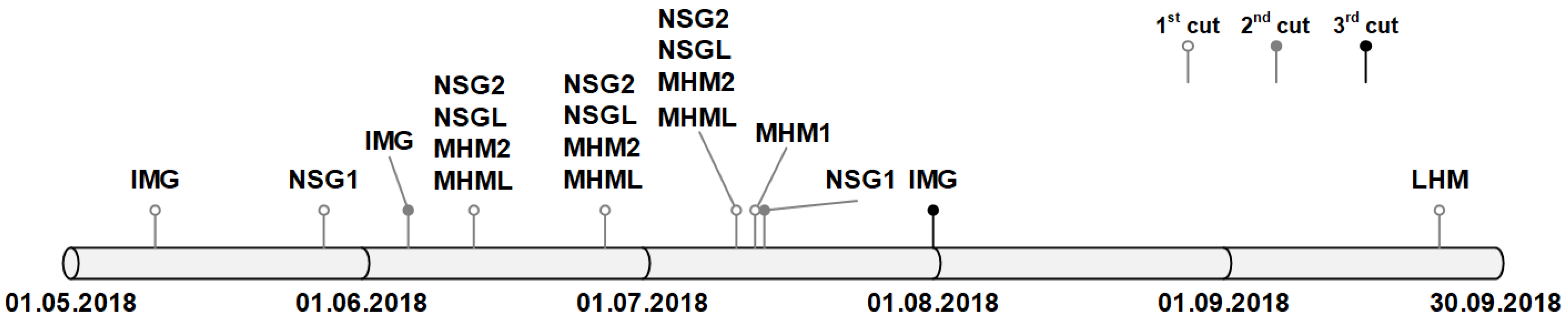
2.2. Biomass Sampling

In all sampling plots (n = 320), the grassland biomass was cut 5 cm above ground level (AGL), and the fresh matter yield (FMY) was weighted directly in the field. A representative biomass subsample was subsequently dried for 48 h at 105 °C, with the dry matter yield (DMY) being calculated subsequently. The biomass sampling was conducted at different dates throughout the growing season in 2018 (Figure 2).

2.3. Hyperspectral Imaging

Hyperspectral image acquisition was conducted using a UAV-borne Cubert FireflEYE S185 (Cubert GmbH, Ulm, Germany) hyperspectral snapshot camera at every grassland site before biomass samples were taken. The sensor is a 2D imaging spectrometer that can detect radiation within a spectral range from 450 to 998 nm. It has 138 spectral bands with a 4 nm sampling interval for each band at 8 nm spectral resolution [22]. The spatial resolution of the sensor is 50 × 50 pixels for each hyperspectral band and 1000 × 1000 pixels for the panchromatic band, while the radiometric resolution is 8 bit.

A Copter Squad RTK-X8 (Copter Squad GmbH, Ulm, Germany) coaxial octocopter UAV was utilized as a platform to carry the hyperspectral sensor. With the sensor mounted onto the stabilized gimbal, the platform provides a flight time of 20 min. The UAV was equipped with a real-time kinematic (RTK) global navigation satellite system (GNSS), allowing flights with centimeter-level accuracy. Flights were conducted at a flight height of 20 m AGL, resulting in a ground sampling distance (GSD) of 20 cm (hyperspectral). During all flights, the heading of the sensor–platform combination was kept constant.

For radiometric calibration of the sensor, a 10 × 10 cm SphereOptics Zenith Lite Diffuse Reflectance Target (SphereOptics GmbH, Herrsching, Germany) was placed under the lens before each flight. Dark calibration was achieved by closing the lens with the lens cap. Georeferencing and orthorectification of the hyperspectral imagery were supported by employing six 1 m² wooden ground control point (GCP) targets, painted in a checkered pattern, distributed at each sampling site. The GCPs were positioned outside the sampling plots with one GCP placed on the short side and two GCPs placed on the long side of the rectangularly shaped plots each. The position of the GCPs was determined with an RTK GPS at a precision of 2 cm.

2.4. Data Processing

The creation of hyperspectral georeferenced orthomosaic image stacks from raw hyperspectral imagery can be divided into three processing steps utilizing different software. In the first step, the raw hyperspectral image cubes were exported from the camera using the software CubeExport DOS (Cubert GmbH, Germany). Afterward, all hyperspectral bands (50 × 50 pixels) were stacked together with the panchromatic band (1000 × 1000 pixel). Secondly, resampling of the 50 × 50 pixels hyperspectral images to 1000 × 1000 pixels applying nearest-neighbor interpolation was carried out using the statistics software R [23]. Resampling to a higher spatial resolution was necessary for precise placement of the markers during georeferencing and followed the procedure described in [17]. The third step comprised stitching the single hyperspectral images to a georeferenced orthomosaic using the software Agisoft PhotoScan Professional (Agisoft LLC, St. Petersburg, Russia). The sparse point cloud generated from the hyperspectral imagery was optimized and georeferenced utilizing precise locational data of the GCPs. The final product was a georeferenced orthomosaic of the study plot containing 138 hyperspectral bands as well as the panchromatic band with a spatial resolution of 20 cm. Subsequently, the pixel values of all spectral bands of the 1 m² subplots were clipped from the georeferenced orthomosaics, and the mean reflectance value for every spectral band was calculated as input for the statistical analysis. From the total of 138 bands, the wavelength portions of 450 to 478 nm (8 bands) and 954 to 998 nm (12 bands) were not used due to noise in this spectral region originating from the sensor’s technical characteristics. The resulting 118 bands ranging from 482 to 950 nm were utilized for data analysis.

2.5. Data Analysis

At first, the spectral reflectance curves of all subplots were normalized using the function normalise.vector (Equation (1)) from statistics software R [23] package ppls [24] in order to reduce the impact of differences in incident radiation between different sampling dates and sites.

$${\tilde{x}}_i=\frac{x_i}{\sqrt{\sum {\Vert x_i\Vert }^2}}$$

(1)

with $x_i$ being the spectral vector for i = 1, 2, …, n.

Secondly, a pre-selection of variables was conducted using the VSURF (variable selection using random forest) function from the VSURF package [19] to reduce data redundancy and increase model parsimony. VSURF was selected as it has been identified as the superior feature selection method regarding performance measures for datasets with many explanatory variables (i.e., wavebands) [25] as proven in multiple studies using ML for modeling from UAV-borne imagery [10,26,27,28]. The VSURF function is a three-step variable selection procedure using random forests (RFs). In the first step, all variables (n = 118) are ranked according to the importance of 50 RF runs. The second step consists of nested RF models (25 runs) involving the most important variables from the first step. The model with the lowest OOB (out-of-bag) error was selected. The third step is a stepwise RF selection of the remaining variables, whereby additional variables are only included when the OOB error decreases significantly compared to the average variation obtained by adding noisy variables [19]. The selected spectral bands from the VSURF were utilized for model building employing four different machine learning (ML) methods (Figure 3).

ML methods were employed due to their ability to handle multicollinear data, such as the contiguous bands of hyperspectral data. The following well established and frequently used ML methods were evaluated for their modeling performance: partial least squares regression (PLSR), support vector regression (SVR), random forest regression (RFR) and Cubist regression (CBR). PLSR is an algorithm searching for a set of latent variables, which represent the covariance between the explanatory variables (i.e., selected waveband) and the response variables (i.e., biomass) best. Latent variables are only added to the model if the error is reduced. The maximum number of latent variables was limited to 20 to reduce the effect of overfitting. SVR is a kernel-based statistical approach, which uses a radial basis function to fit the data to a hyperplane [29]. SVR is beneficial for fitting complex non-linear data. The optimal model was identified using a systematic grid search, tuning the cost and sigma parameter [30]. RFR, a tree-based ensemble learning technique, combines the information from many variables. In this study, the number of trees was kept at 500 [31] independent decision trees [32]. For identifying the optimal model, the parameter mtry (defining the number of randomly selected variables at each split in the regression tree) was tuned. The minimum node size was kept at five [33]. CBR is a rule-based regression technique that retrieves a set of rules with sets of multivariate models [34,35]. The best model selection is based on rules that best fit an explicit set of predictors [36,37]. For tuning the CBR model, the best combination of the parameter’s committees and neighbors were searched. The model building process was carried out using the caret package (version 6.0.85) [38] in statistics software R. Spectral data and the target variables FMY and DMY were utilized as input for the modeling process (Figure 3).

All samples were randomly split into two portions: 80% of the samples were used for calibration, and 20% of the samples were used for validation, using grassland site and sampling date as a stratum. The ratio of 80% to 20% was chosen to utilize a high proportion of the samples in the calibration process to achieve a good model fit while still retaining a considerable number of 64 samples in the validation. As a specific set of calibration samples can alter the modeling result, a random split of calibration and validation samples was repeated 100 times (Figure 3) to reduce the impact of particular samples on model performance.

Model calibration was carried out by applying k-fold cross-validation with 10 folds and 5 repetitions. The best tuning parameters were chosen based on the model performance in the cross-validation and were measured by the metric RMSE. As every model was repeated 100 times, 100 best tuning parameters were determined (Figure 3). The validation model performance was measured by median values (median of 100 iterations) of the performance metrics R², RMSE_p and nRMSE_p (Equations (2)–(4)). Based on the best median model performance, the best algorithm for FMY and DMY prediction from the hyperspectral dataset was determined.

The most frequently identified best tuning parameters (i.e., median of 100 tuned models) were identified for the best ML approach in the final step. The identified tuning parameters were subsequently used to calibrate the final model with all 320 samples. The normalized deviation (Equation (5)) was calculated for all samples to examine this final model’s potential deviations regarding grassland type and sampling date. Values close to zero indicate good prediction accuracies. Furthermore, a Wilcox test [39] was applied to test whether the deviations from zero were statistically significant.

$$R_P^2=\left[1-\frac{{{\displaystyle \sum }}_{i=1}^n{\left(y_i-{\widehat{y}}_i\right)}^2}{{{\displaystyle \sum }}_{i=1}^n{\left(y_i-{\overline{y}}_i\right)}^2}\right]$$

(2)

$$RMS{E}_P=\sqrt{\frac{{{\displaystyle \sum }}_{i=1}^n{\left({\widehat{y}}_i-y_i\right)}^2}{n}}$$

(3)

$$nRMSE=\frac{RMS{E}_{val}}{\max \left(y_i\right)-\min \left(y_i\right)}$$

(4)

$$\begin{array}{c}\mathrm{Normalized}\mathrm{deviation}=\frac{{\widehat{y}}_i-y_i}{y_i+{\widehat{y}}_i} \end{array}$$

(5)

where y_i is the measured biomass, ${\widehat{y}}_i$ is the predicted biomass, ${\overline{y}}_i$ is the average measured biomass and n is the number of samples.

3. Results

3.1. Biomass Data

Aggregated data of FMY and DMY of the sampled grasslands were featured by an extensive range of values (4.06 and 0.61 kg/m² respectively,

Table 2. Overview of aggregated FMY and DMY biomass (kg/m²) data (n = 320).

Statistic	FMY (kg/m2)	DMY (kg/m2)
Mean	0.69	0.19
Median	0.53	0.17
Min.	0.01	0.01
Max.	4.07	0.62
Standard deviation	0.73	0.14
Coefficient of variation	105%	72%

) and a high coefficient of variation (105% and 72%). This was expected due to different management intensities and grassland types. Additionally, the dry weather resulted in meagre biomass yields during the second and third cuts (See Appendix A,

Table A1. Median FMY and DMY biomass yield per cutting date. At grassland sites NGS2, NSGL, MHM2 and MHML different areas of the plot were cut at three sampling dates, resulting in differing dates for the first cut.

Grassland Site	Number of Cuts	Median FMY (kg/m2)	Median DMY (kg/m2)
MHM1	1st	0.36	0.14
NSG1	1st	0.05	0.03
LHM	1st	0.89	0.27
	2nd	0.09	0.04
IMG	1st	2.95	0.47
	2nd	0.22	0.05
	3rd	0.17	0.06
NSG2	1st	0.13	0.06
	1st	0.13	0.05
	1st	0.28	0.11
NSGL	1st	0.84	0.24
	1st	0.73	0.23
	1st	0.72	0.29
MHM2	1st	1.06	0.29
	1st	1.04	0.33
	1st	1.13	0.36
MHML	1st	0.72	0.21
	1st	0.61	0.19
	1st	0.98	0.33

). The highest FMY and DMY was recorded at the most intensively managed, fertilized grassland (IMG). The extensive nature of all other grasslands is evident from their low DMY yields ranging from 0.03 to 0.36 kg/m² (See Appendix A, Table A1).

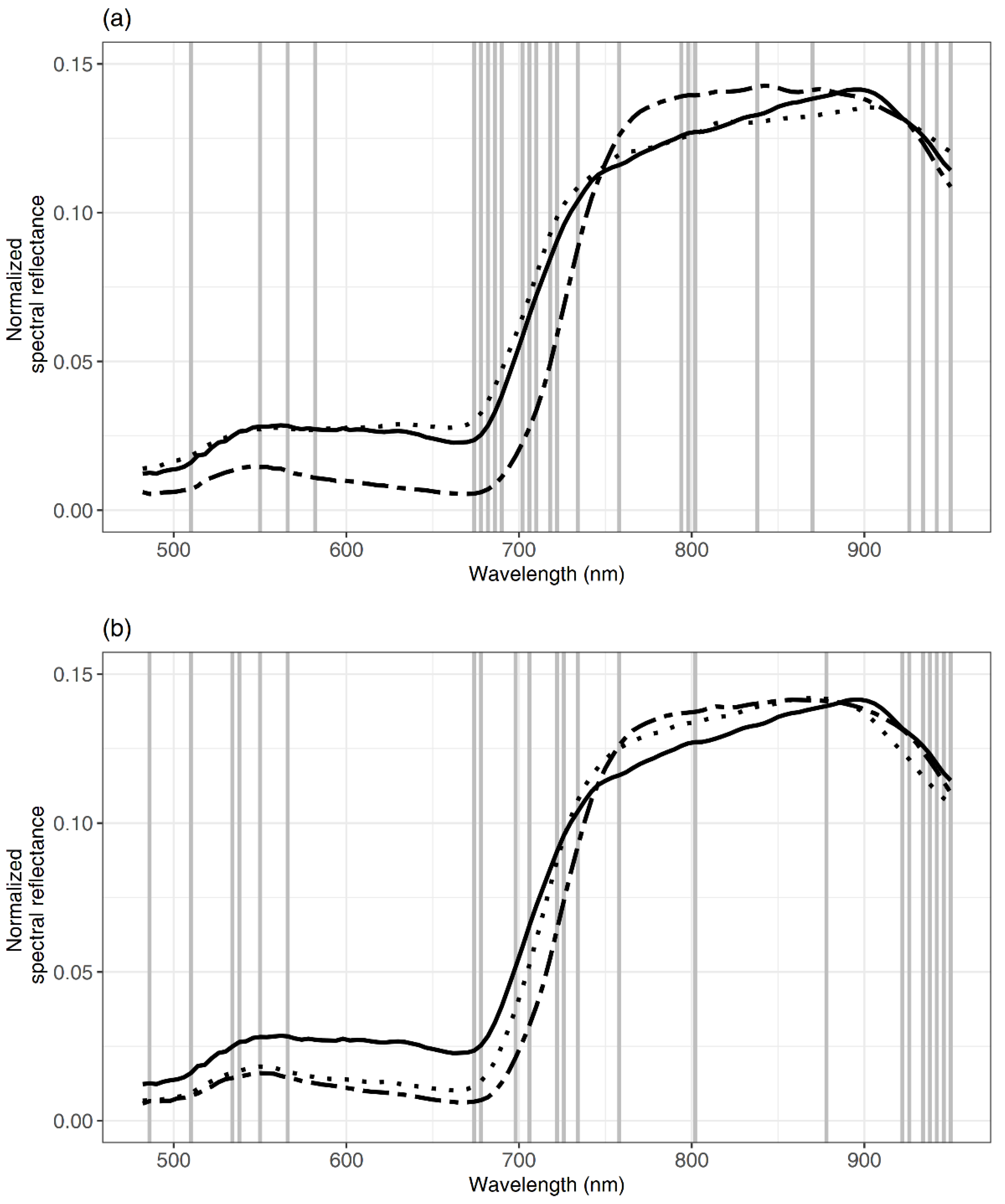
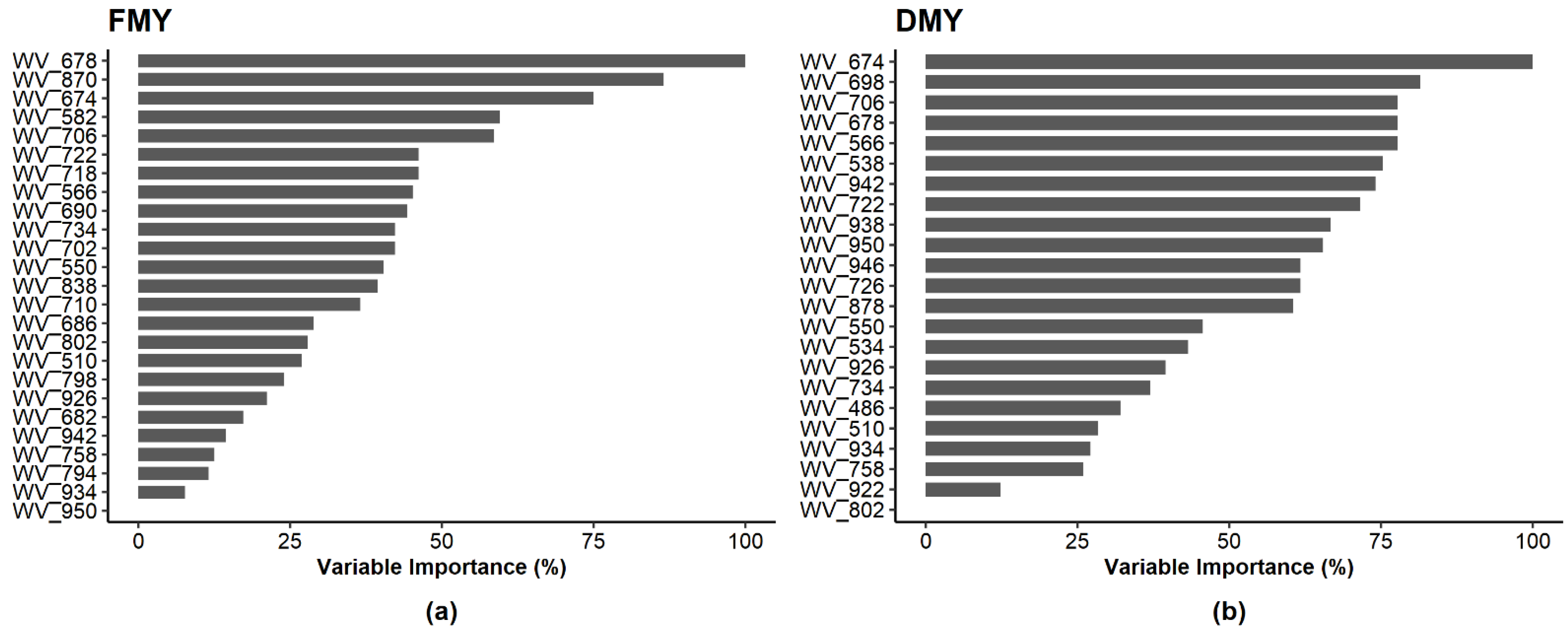
3.2. Spectral Data and Selected Spectral Bands

Normalized spectra depicted typical reflectance signatures of green vegetation (Figure 4). Plots with high biomass values were featured by low reflectance in the red spectral region and high reflectance in the near infrared (NIR) (Figure 4). Low reflectance in the red most likely resulted from high absorption from leaf pigments, mainly chlorophyll, while high reflectance in the NIR can be explained by strong reflectance in the spongy mesophyll of plant leaves [40]. Both effects point to a high amount of leaf biomass per area and indicate high FMY and DMY yield.

The band selection for FMY and DMY using VSURF reduced the number of spectral bands. For FMY and DMY, 25 and 23 wavebands were selected. The identified most important wavebands for FMY and DMY were in the same spectral regions and covered all spectral regions (visible: 400–750 nm, red edge: 680–730 nm, and NIR: 780–950 nm) known for being related to green biomass [40]. The most important wavelengths selected (Figure 5) were centered around the red edge and the green spectral regions (530–590 nm). These regions are especially sensible for changes in cell structure and leaf pigment concentrations and, therefore, well known for their high importance in grassland biomass modeling. For DMY modeling, wavelengths above 930 nm were of high importance, likely reflecting the information on water content from a minor water absorption band in this spectral region [41].

3.3. Performance of Modeling Algorithms

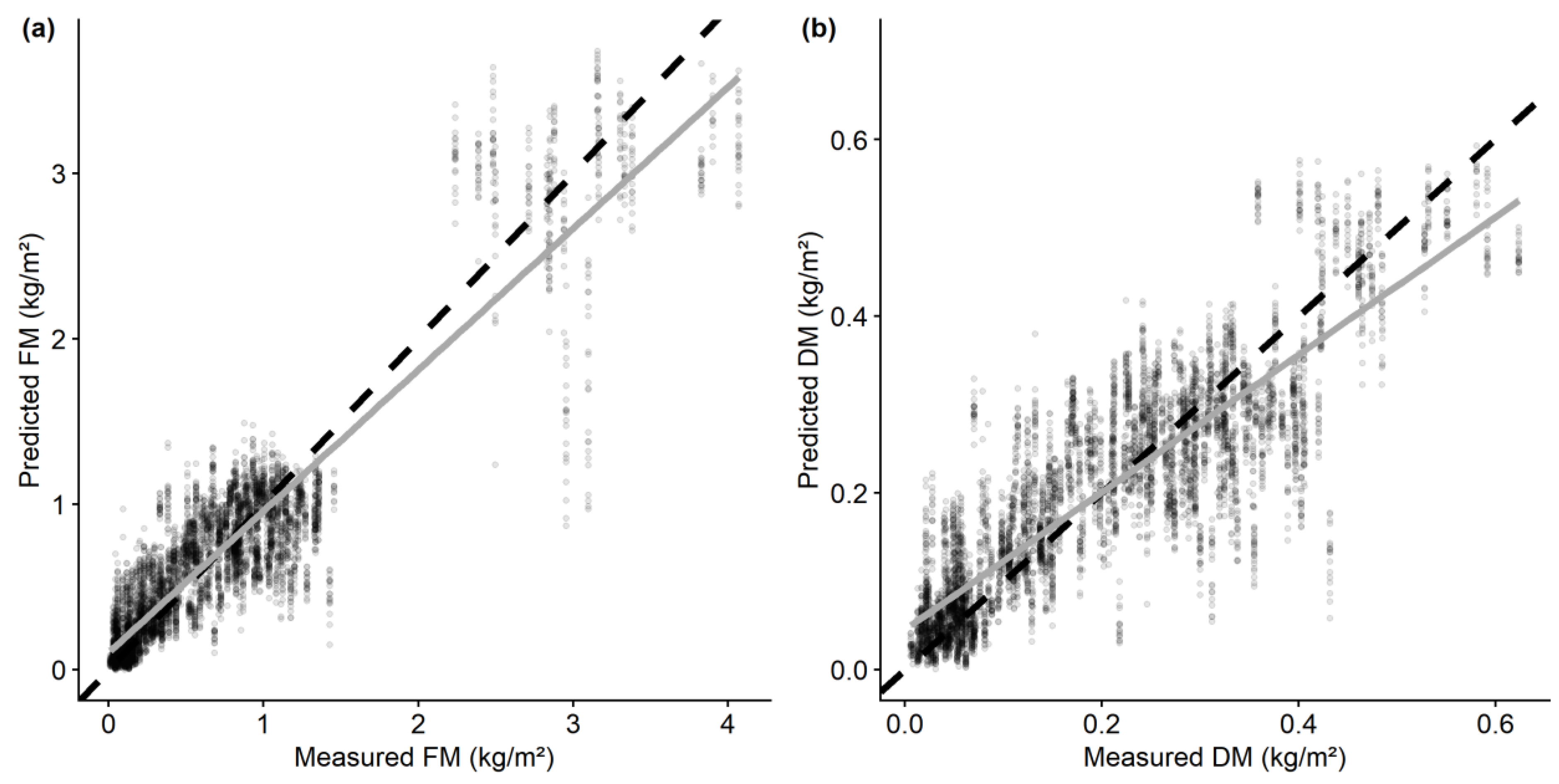
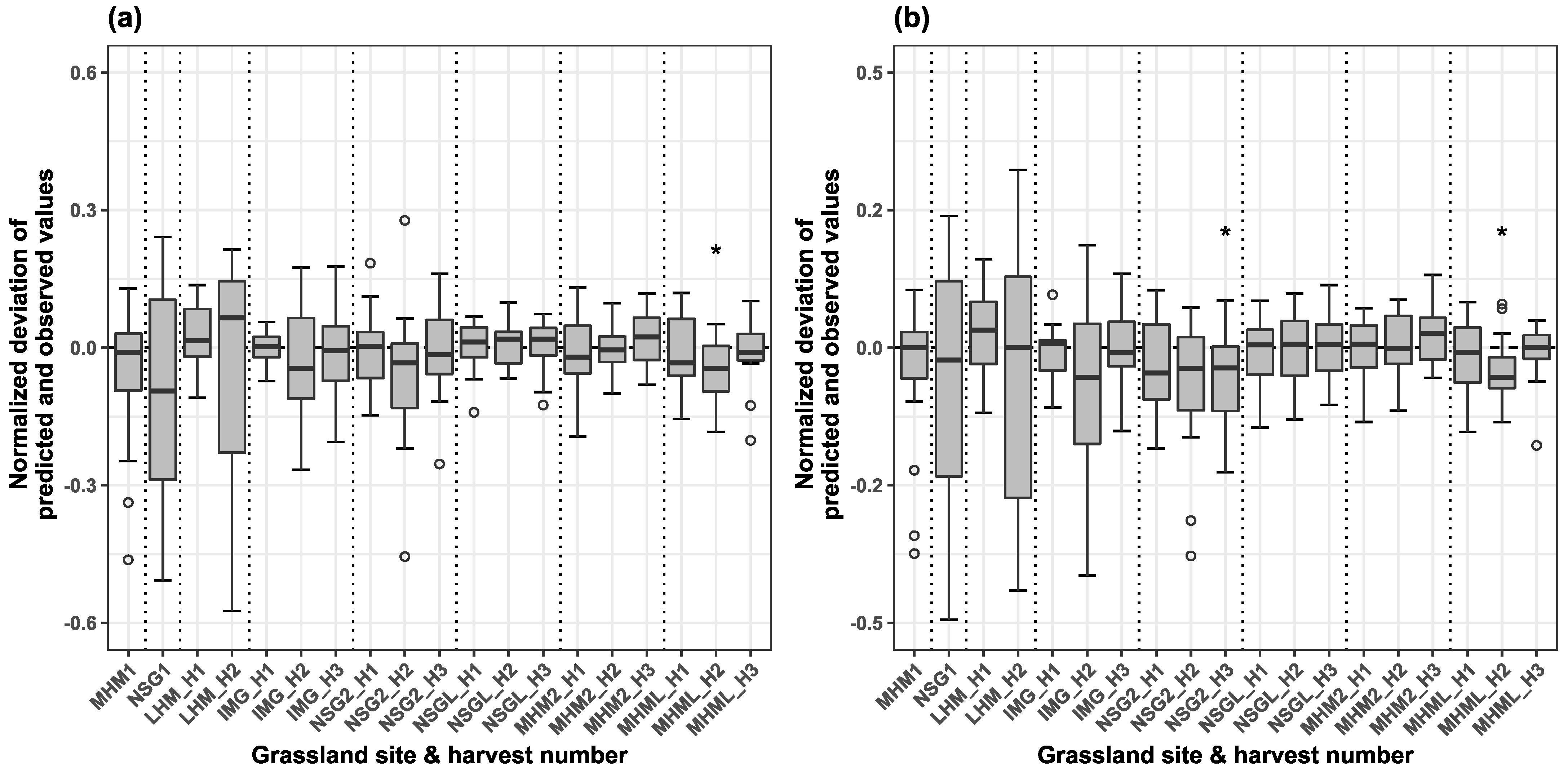
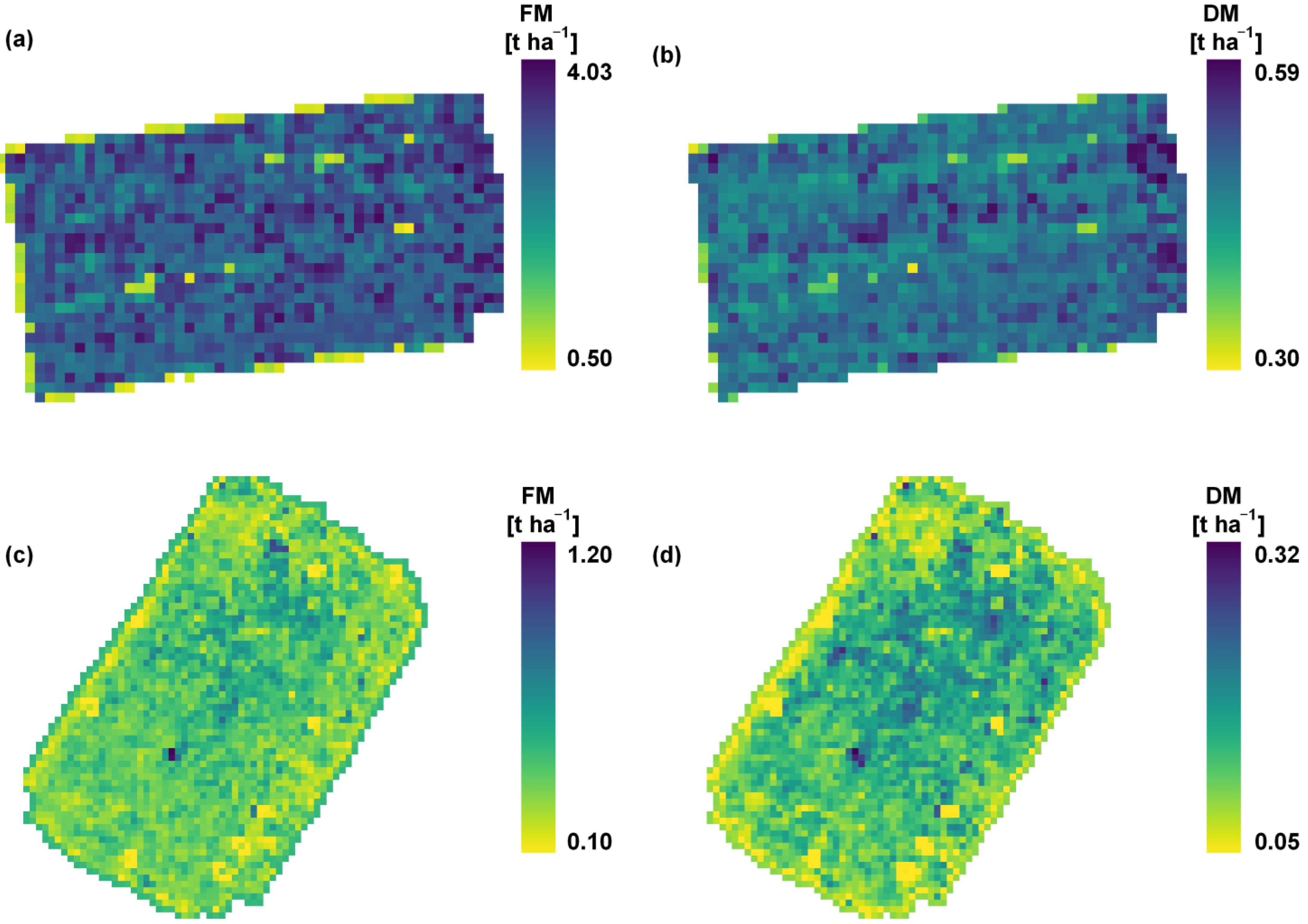
The evaluation of median modeling performances of the ML algorithms revealed that CBR performed best for FMY as well as for DMY modeling with the lowest median relative error (nRMSE_p) of 7.6% and 12.9%, respectively, as well as the lowest median RMSE_p (0.27 and 0.07 kg/m²) and the highest coefficient of determination ($R_p^2$, 0.87 and 0.75). However, the differences in median modeling performance between RFR, SVR and CBR were negligible. Only PLSR performed distinctly poorer than all other modeling algorithms. All algorithms could predict both grassland FMY and DMY with a low relative error, ranging from 7.6% to 11.9% and 12.9% to 18.9%, respectively (

Table 3. Performance of different ML algorithms for FMY and DMY modeling. Performance figures are median values of 100 iterations with different random sample splits for calibration and validation. The best model is indicated by bold text.

	Algorithm	$\mathbf{Median}{\mathbf{R}}_{\mathbf{p}}^2$	Median RMSEp (kg/m2)	SD RMSEp (kg/m2)	Median nRMSEp
FMY (kg/m2)	PLSR	0.68	0.42	0.04	11.9%
	RFR	0.85	0.29	0.04	8.0%
	SVR	0.86	0.29	0.03	7.9%
	CBR	0.87	0.27	0.05	7.6%
DMY (kg/m2)	PLSR	0.45	0.10	0.01	18.9%
	RFR	0.73	0.07	0.01	13.5%
	SVR	0.74	0.07	0.01	13.0%
	CBR	0.75	0.07	0.01	12.9%

).

The observed versus predicted plot of the CBR model for FMY (Figure 6a) revealed the FMY yield difference between the intensively managed grassland (IMG) with high biomass values and all other grasslands. The deviation of the values from the 1:1 line increased for higher FMY yields. For DMY, higher variation could be found in the medium biomass values between 0.3 and 0.4 kg/m² (Figure 6b).

3.4. Final Model

The identified best ML approach (CBR) can subsequently be used for map creation and, thus, was finally calibrated using 10-fold cross-validation using the complete dataset (n = 320) and the tuning parameter derived from the median best models (committees = 95 and 96, neighbors = 3 and 4 for FMY and DMY, respectively). The final model’s errors were close to the median error from the 100 model validation runs in the model tuning phase (RMSE_P = 0.27 and 0.07 kg/m², $R_P^2$ = 0.85 and 0.76 for FMY and DMY, respectively). An analysis of the normalized deviation of the predicted from the observed biomass values (Figure 7) from zero revealed only significant deviations for the lupin-invaded grassland MHML at harvest two (FMY and DMY) and harvest three at grassland NSG2 (DMY). FMY estimation of the sites NSG1 and LHM at harvest two showed high normalized deviations of predicted from observed values, although these were not significant. The deviations likely result from the very low FMY values found at these sites during the respective harvest, which was influenced by severe drought. Thus, these values mark the lower end of FMY values and were difficult to predict with a model trained predominantly from hyperspectral reflectance data from fields with much higher FMY values. No systematic and significant deviations for any grassland site or harvest date were found, indicating the model’s robustness.

The final model can map FMY and DMY values at a spatial resolution of 1 m² (Figure 8). These maps could finally be used for the spatiotemporal, explicit interpretation of biomass distributions. For example, the most intensively used grassland (Figure 8a,b) showed a more extensive range for FMY values, while DMY values varied more strongly at an extensively managed grassland (MHM1) during the first sampling date (Figure 8c,d). In both maps, areas with disturbed sward feature distinctly different FMY and DMY values, enabling their remote detection. The maps for grassland site IMG reveal possible management-related effects on DMY and FMY evident from a stripe pattern following the main driving direction on the field from east to west (Figure 8a,b). At grassland site MHM1, the highest biomass yield was found in the northeastern part of the plot (Figure 8c,d) where increasing terrain height on a southbound oriented slope could have led to increased sun exposure and, thus, improved grassland growth conditions.

4. Discussion

The primary aim of this study was to retrieve UAV-based models for estimation of the forage yield of eight grassland sites along a gradient of management intensities. In previous studies, grassland biomass could be predicted from UAV-borne RGB 3D point cloud [8,42], multispectral [43] and hyperspectral data [11], as well as through fusion of these sensors [10,26] with good accuracies. However, the majority of these studies were carried out at experimental plots incorporating few different grassland plant communities and management regimes, limiting their practical significance. The present study, thus, aimed at the development of a robust model that can be applied to a wide range of grassland usage intensities as found in practical farming in Central Germany.

The workflow proposed and the applied optimization procedure based on waveband selection, ML model identification and ML tuning led to low prediction errors and, thus, high model accuracies for FMY and DMY prediction (nRMSE_p 7.6% and 12.9% for FMY and DMY). In the first step, the wavebands most important for predicting FMY and DMY were selected using the VSURF method. The number of wavebands could be reduced by around 80% for both biomass parameters, increasing the model simplicity and reducing the risk of overfitting when used in conjunction with ML methods known for their ability to deal with multicollinear data with a small number of samples. Although the remaining number of variables remained high (25 and 23 for FMY and DMY, respectively), the workflow of 100 model iterations with different samples from all sites and sampling dates selected for calibration and validation likely reduced the impact of single samples from the dataset. Model performance was given as median values of 100 model runs, thus reducing the risk of overoptimistic results. Further research could identify possible improvements in variable reduction, i.e., model simplification, through the employment of different reduction methods such as filtering variables by a variable importance in the projection (VIP) threshold. However, that method delivered unsatisfactory results in a study on estimation of the quality parameter starch content of the grassland species red clover from hyperspectral data [44]. Another promising method for variable reduction in ML approaches previously employed on grassland data is the Boruta algorithm [45]. Due to its high computational intensity [46], however, Boruta was ruled out for the present study. With the aim of simplification and increased practical applicability, in a separate approach, the number of wavebands could be downsampled to 5–10 bands (multispectral) to compare the modeling accuracy with reduced variables available.

For both FMY and DMY, the selected wavebands were in similar regions of the electromagnetic spectrum (Figure 4). While for FMY prediction, more wavebands were selected in the red edge region (750–780 nm), known for being related to LAI, biomass and leaf internal structure [47], more wavebands in the NIR region beyond 920 nm were selected for DMY prediction. This spectral region is related to the water content of biomass [40,48]. Overall, the identified wavebands coincide with current knowledge about relationships between vegetation biomass and spectral reflectance [40,49]. Model accuracy for FMY prediction was higher than for DMY, likely depicting the closer relationship of FMY to measured reflectance above the canopy of plants containing considerable amounts of water. During the dry weather in 2018, high amounts of dry plant material might have obscured the relationship between reflectance and DMY more than with FMY. In dry plots, e.g., some portion of DMY may not have been detectable from UAV-borne imagery due to low reflectance from dried plant material. Additionally, a higher variation of values for FMY (Table 2) could have improved the ability of ML algorithms to model FMY from hyperspectral reflectance.

Four ML algorithms were evaluated to identify the one most suitable for predicting FMY and DMY. Testing multiple ML algorithms has been identified as helpful and was recommended by several studies as no ML approach always performs best [50,51,52]. In the present study, CBR showed the best performance for FMY and DMY prediction from hyperspectral data (Table 3). However, the differences in comparison to RFR and SVR were minor. PLSR was outperformed by the three other approaches coinciding with the results of previous studies [9,50]. The advantage of CBR, RFR and SVR is the ability to model non-linear relationships between the response (i.e., FMY, DMY) and explanatory variables (i.e., wavebands) [53,54]. Overall, the model accuracies received in the present study are in the upper range of recent grassland biomass prediction models using remote sensing data [5,55]. Psomas et al. [55], for example, also examined four grassland types and one complete growing season. The best model, similarly, based on band selection but linear regression approaches, was feature a relative prediction error of 8.5%, which is slightly worse than in the present study. However, the reflectance information was collected using a field spectrometer. In comparison to UAV-borne data, field spectrometer data are less affected by external factors such as light incidence angle or wind, but on the other hand also less applicable to large areas.

The final models showed no systematic deviation of the predicted from the observed values related to grassland site or sampling date (Figure 6 and Figure 7). However, the values should not be over-interpreted as the stability of the prediction results is based on the final calibration model only, and a validation with an external dataset should be the next step to examine limitations of the prediction capabilities of the models.

Overall, the study showed that it is possible to calibrate remote sensing models for estimating grassland biomass along a gradient of management intensities. To the best knowledge of the authors, this is the first study covering multiple sites with different management intensities along a whole growing period using hyperspectral UAV-borne data. Thus, the study may contribute to closing the gap between grassland biomass estimation on agricultural plot trials and application on practical grassland sites, although the workflow established in this study far from being suitable for practical farming. However, the stability of the prediction models in this study showed, as for every empirical model, that limitations arose when biomass should be predicted for grasslands with biomass values far away from the mean (in this study, high biomass values: 4.0 and 0.62 kg/m² for FMY and DMY). These limitations could be reduced by the inclusion of additional data from other grassland sites in the model calibration. Additional data could only be used in the model calibration process if they originated from a hyperspectral sensor with similar technical characteristics such as spectral bandwidth and number of wavebands, though. In a following step, the model should be validated across multiple years to test its stability under changing growing conditions. Nevertheless, the aim of the study was not to develop a generalized model applicable on all conditions and grasslands but rather to examine the potential of hyperspectral UAV-borne data to successfully predict biomass for grasslands with different management intensities. For improved practical applicability, models similar to the one developed in this study should be validated on a range of grassland sites from different regions and years. This could be supported by using data from other experiments, as well as practice research networks. Although hyperspectral sensors offer advantages for the modeling of grassland traits through their high spectral resolution, their cost and difficult operation restrict them from widespread application in grassland monitoring for practical farming. Future studies, thus, should test whether results similar to the estimation of grassland biomass from hyperspectral imagery can be retrieved from multispectral sensors under the same practical circumstances (i.e., usage intensities, plant communities). Apart from restrictions regarding sensor technology and data processing, low profits from extensive grassland farming (reducing demand) coupled with the requirement to operate UAVs only within one’s line of sight (increasing cost per area) remain obstacles for the application of UAV-borne data in practical grassland biomass estimation.

In future, empirical models similar to the one developed could be coupled with mechanical models such as APSIM [56] to compensate for the limitations of both modeling approaches (i.e., generalizability for empirical models and temporally and spatially continuous reference data for mechanical models). In order to improve model accuracies, fusion approaches with, e.g., structural information derived from point clouds [10,26] could be used. Additionally, new statistical approaches such as deep learning show great potential for improving the prediction of vegetation parameters [57].

In conclusion, the present study has shown the great potential of hyperspectral UAV-borne data for retrieving information on biomass yield of grassland in a spatially continuous way throughout the whole growing period. Although not ready for practical application in grassland management, the accuracies of the models indicate that it is possible to map the biomass yield of grasslands over a wide range of management intensities.

References

1. Smit, H.J.; Metzger, M.J.; Ewert, F. Spatial Distribution of Grassland Productivity and Land Use in Europe. Agric. Syst. 2008, 98, 208–219. [Google Scholar] [CrossRef]
2. Wachendorf, M.; Fricke, T.; Möckel, T. Remote Sensing as a Tool to Assess Botanical Composition, Structure, Quantity and Quality of Temperate Grasslands. Grass Forage Sci. 2018, 73, 1–14. [Google Scholar] [CrossRef]
3. Harmoney, K.R.; Moore, K.J.; George, J.R.; Brummer, E.C.; Russell, J.R. Determination of Pasture Biomass Using Four Indirect Methods. Agron. J. 1997, 89, 665–672. [Google Scholar] [CrossRef]
4. Hakl, J.; Hrevušová, Z.; Hejcman, M.; Fuksa, P. The Use of a Rising Plate Meter to Evaluate Lucerne (Medicago sativa L.) Height as an Important Agronomic Trait Enabling Yield Estimation. Grass Forage Sci. 2012, 67, 589–596. [Google Scholar] [CrossRef]
5. Reinermann, S.; Asam, S.; Kuenzer, C. Remote Sensing of Grassland Production and Management—A Review. Remote Sens. 2020, 12, 1949. [Google Scholar] [CrossRef]
6. Safari, H.; Fricke, T.; Reddersen, B.; Möckel, T.; Wachendorf, M. Comparing Mobile and Static Assessment of Biomass in Heterogeneous Grassland with a Multi-Sensor System. J. Sens. Sens. Syst. 2016, 5, 301–312. [Google Scholar] [CrossRef] [Green Version]
7. Stumpf, F.; Schneider, M.K.; Keller, A.; Mayr, A.; Rentschler, T.; Meuli, R.G.; Schaepman, M.; Liebisch, F. Spatial Monitoring of Grassland Management Using Multi-Temporal Satellite Imagery. Ecol. Indic. 2020, 113, 106201. [Google Scholar] [CrossRef]
8. Wijesingha, J.; Moeckel, T.; Hensgen, F.; Wachendorf, M. Evaluation of 3D Point Cloud-Based Models for the Prediction of Grassland Biomass. Int. J. Appl. Earth Obs. Geoinf. 2019, 78, 352–359. [Google Scholar] [CrossRef]
9. Grüner, E.; Wachendorf, M.; Astor, T. The Potential of UAV-Borne Spectral and Textural Information for Predicting Aboveground Biomass and N Fixation in Legume-Grass Mixtures. PLoS ONE 2020, 15, e0234703. [Google Scholar] [CrossRef]
10. Schulze-Brüninghoff, D.; Wachendorf, M.; Astor, T. Remote Sensing Data Fusion as a Tool for Biomass Prediction in Extensive Grasslands Invaded by L. polyphyllus. Remote Sens. Ecol. Conserv. 2021, 7, 198–213. [Google Scholar] [CrossRef]
11. Näsi, R.; Viljanen, N.; Kaivosoja, J.; Alhonoja, K.; Hakala, T.; Markelin, L.; Honkavaara, E. Estimating Biomass and Nitrogen Amount of Barley and Grass Using UAV and Aircraft Based Spectral and Photogrammetric 3D Features. Remote Sens. 2018, 10, 1082. [Google Scholar] [CrossRef] [Green Version]
12. Oliveira, R.A.; Näsi, R.; Niemeläinen, O.; Nyholm, L.; Alhonoja, K.; Kaivosoja, J.; Jauhiainen, L.; Viljanen, N.; Nezami, S.; Markelin, L.; et al. Machine Learning Estimators for the Quantity and Quality of Grass Swards Used for Silage Production Using Drone-Based Imaging Spectrometry and Photogrammetry. Remote Sens. Environ. 2020, 246, 111830. [Google Scholar] [CrossRef]
13. Geipel, J.; Korsaeth, A. Hyperspectral Aerial Imaging for Grassland Yield Estimation. Adv. Anim. Biosci. 2017, 8, 770–775. [Google Scholar] [CrossRef]
14. Kong, B.; Yu, H.; Du, R.; Wang, Q. Quantitative Estimation of Biomass of Alpine Grasslands Using Hyperspectral Remote Sensing. Rangel. Ecol. Manag. 2019, 72, 336–346. [Google Scholar] [CrossRef]
15. Lussem, U.; Bolten, A.; Menne, J.; Gnyp, M.L.; Schellberg, J.; Bareth, G. Estimating Biomass in Temperate Grassland with High Resolution Canopy Surface Models from UAV-Based RGB Images and Vegetation Indices. J. Appl. Remote Sens. 2019, 13, 034525. [Google Scholar] [CrossRef]
16. Capolupo, A.; Kooistra, L.; Berendonk, C.; Boccia, L.; Suomalainen, J. Estimating Plant Traits of Grasslands from UAV-Acquired Hyperspectral Images: A Comparison of Statistical Approaches. ISPRS Int. J. Geo-Inf. 2015, 4, 2792–2820. [Google Scholar] [CrossRef]
17. Wijesingha, J.; Astor, T.; Schulze-Brüninghoff, D.; Wengert, M.; Wachendorf, M. Predicting Forage Quality of Grasslands Using UAV-Borne Imaging Spectroscopy. Remote Sens. 2020, 12, 126. [Google Scholar] [CrossRef] [Green Version]
18. Clevers, J.G.P.W.; van der Heijden, G.; Verzakov, S.; Schaepman, M.E. Estimating Grassland Biomass Using SVM Band Shaving of Hyperspectral Data. Photogramm. Eng. Remote Sens. 2007, 73, 1141–1148. [Google Scholar] [CrossRef] [Green Version]
19. Genuer, R.; Poggi, J.-M.; Tuleau-Malot, C. VSURF: An R Package for Variable Selection Using Random Forests. R J. 2015, 7, 19–33. [Google Scholar] [CrossRef] [Green Version]
20. Kursa, M.B.; Rudnicki, W.R. Feature Selection with the Boruta Package. J. Stat. Softw. 2010, 36, 1–13. [Google Scholar] [CrossRef] [Green Version]
21. Löns-Hanna, C.; Kremer, M.; Rittershofer, B. Niedrigwasser und Trockenheit. 2018. Hess. Landesamt Für Nat. Umw. Geol. 2019, 1, 1–21. [Google Scholar]
22. Cubert GmbH FireflEYE SE–Hyperspectral Camera. Cubert. S185–Hyperspectral SE. Available online: https://cubert-gmbh.com/ (accessed on 16 April 2022).
23. R Core Team. R: A Language and Environment for Statistical Computing; R Foundation for Statistical Computing: Vienna, Austria, 2021. [Google Scholar]
24. Kraemer, N.; Boulesteix, A.-L.; Tutz, G. Penalized Partial Least Squares with Applications to B-Spline Transformations and Functional Data. Chemom. Intell. Lab. Syst. 2008, 94, 60–69. [Google Scholar] [CrossRef] [Green Version]
25. Speiser, J.L.; Miller, M.E.; Tooze, J.; Ip, E. A Comparison of Random Forest Variable Selection Methods for Classification Prediction Modeling. Expert Syst. Appl. 2019, 134, 93–101. [Google Scholar] [CrossRef] [PubMed]
26. Grüner, E.; Astor, T.; Wachendorf, M. Prediction of Biomass and N Fixation of Legume-Grass Mixtures Using Sensor Fusion. Front. Plant Sci. 2021, 11, 2192. [Google Scholar] [CrossRef]
27. Wengert, M.; Piepho, H.-P.; Astor, T.; Graß, R.; Wijesingha, J.; Wachendorf, M. Assessing Spatial Variability of Barley Whole Crop Biomass Yield and Leaf Area Index in Silvoarable Agroforestry Systems Using UAV-Borne Remote Sensing. Remote Sens. 2021, 13, 2751. [Google Scholar] [CrossRef]
28. Schulze-Brüninghoff, D.; Wachendorf, M.; Astor, T. Potentials and Limitations of WorldView-3 Data for the Detection of Invasive Lupinus polyphyllus Lindl. in Semi-Natural Grasslands. Remote Sens. 2021, 13, 4333. [Google Scholar] [CrossRef]
29. Cortes, C.; Vapnik, V. Support-Vector Networks. Mach. Learn. 1995, 20, 273–297. [Google Scholar] [CrossRef]
30. Karatzoglou, A.; Meyer, D.; Hornik, K. Support Vector Machines in R. J. Stat. Softw. 2006, 15, 1–28. [Google Scholar] [CrossRef] [Green Version]
31. Probst, P.; Boulesteix, A.-L. To Tune or Not to Tune the Number of Trees in Random Forest? J. Mach. Learn. Res. 2017, 18, 6673–6690. [Google Scholar]
32. Breiman, L. Random Forests. Mach. Learn. 2001, 45, 5–32. [Google Scholar] [CrossRef] [Green Version]
33. Wright, M.N.; Ziegler, A. Ranger: A Fast Implementation of Random Forests for High Dimensional Data in C++ and R. J. Stat. Softw. 2015, 77, 1–17. [Google Scholar] [CrossRef] [Green Version]
34. Quinlan, J.R. Simplifying Decision Trees. Int. J. Hum.-Comput. Stud. 1999, 51, 497–510. [Google Scholar] [CrossRef] [Green Version]
35. Quinlan, J.R. Machine Learning: Proceedings of the Tenth International Conference; University of Massachusetts: Amherst, MA, USA, 1993; pp. 27–29. ISBN 978-1-4832-9862-7. [Google Scholar]
36. Appelhans, T.; Mwangomo, E.; Hardy, D.R.; Hemp, A.; Nauss, T. Evaluating Machine Learning Approaches for the Interpolation of Monthly Air Temperature at Mt. Kilimanjaro, Tanzania. Spat. Stat. 2015, 14, 91–113. [Google Scholar] [CrossRef] [Green Version]
37. Hafeez, S.; Wong, M.S.; Ho, H.C.; Nazeer, M.; Nichol, J.; Abbas, S.; Tang, D.; Lee, K.H.; Pun, L. Comparison of Machine Learning Algorithms for Retrieval of Water Quality Indicators in Case-II Waters: A Case Study of Hong Kong. Remote Sens. 2019, 11, 617. [Google Scholar] [CrossRef] [Green Version]
38. Kuhn, M. Building Predictive Models in R Using the Caret Package. J. Stat. Softw. 2008, 28, 1–26. [Google Scholar] [CrossRef] [Green Version]
39. Bauer, D.F. Constructing Confidence Sets Using Rank Statistics. J. Am. Stat. Assoc. 1972, 67, 687–690. [Google Scholar] [CrossRef]
40. Ollinger, S.V. Sources of Variability in Canopy Reflectance and the Convergent Properties of Plants: Tansley Review. New Phytol. 2011, 189, 375–394. [Google Scholar] [CrossRef]
41. Clevers, J.G.P.W.; Kooistra, L.; Schaepman, M.E. Using Spectral Information from the NIR Water Absorption Features for the Retrieval of Canopy Water Content. Int. J. Appl. Earth Obs. Geoinf. 2008, 10, 388–397. [Google Scholar] [CrossRef]
42. Lussem, U.; Schellberg, J.; Bareth, G. Monitoring Forage Mass with Low-Cost UAV Data: Case Study at the Rengen Grassland Experiment. PFG–J. Photogramm. Remote Sens. Geoinf. Sci. 2020, 88, 407–422. [Google Scholar] [CrossRef]
43. Schucknecht, A.; Seo, B.; Krämer, A.; Asam, S.; Atzberger, C.; Kiese, R. Estimating Dry Biomass and Plant Nitrogen Concentration in Pre-Alpine Grasslands with Low-Cost UAS-Borne Multispectral Data—A Comparison of Sensors, Algorithms, and Predictor Sets. Biogeosciences Discuss. 2021, preprint. [Google Scholar] [CrossRef]
44. Frey, L.; Baumann, P.; Aasen, H.; Studer, B.; Kölliker, R. A Non-Destructive Method to Quantify Leaf Starch Content in Red Clover. Front. Plant Sci. 2020, 11, 1533. [Google Scholar] [CrossRef] [PubMed]
45. Zandler, H.; Faryabi, S.P.; Ostrowski, S. Contributions to Satellite-Based Land Cover Classification, Vegetation Quantification and Grassland Monitoring in Central Asian Highlands Using Sentinel-2 and MODIS Data. Front. Environ. Sci. 2022, 10, 164. [Google Scholar] [CrossRef]
46. Degenhardt, F.; Seifert, S.; Szymczak, S. Evaluation of Variable Selection Methods for Random Forests and Omics Data Sets. Brief. Bioinform. 2019, 20, 492–503. [Google Scholar] [CrossRef] [Green Version]
47. Chen, J.; Gu, S.; Shen, M.; Tang, Y.; Matsushita, B. Estimating Aboveground Biomass of Grassland Having a High Canopy Cover: An Exploratory Analysis of in Situ Hyperspectral Data. Int. J. Remote Sens. 2009, 30, 6497–6517. [Google Scholar] [CrossRef]
48. Riano, D.; Vaughan, P.; Chuvieco, E.; Zarco-Tejada, P.J.; Ustin, S.L. Estimation of Fuel Moisture Content by Inversion of Radiative Transfer Models to Simulate Equivalent Water Thickness and Dry Matter Content: Analysis at Leaf and Canopy Level. IEEE Trans. Geosci. Remote Sens. 2005, 43, 819–826. [Google Scholar] [CrossRef]
49. Kokaly, R.F.; Asner, G.P.; Ollinger, S.V.; Martin, M.E.; Wessman, C.A. Characterizing Canopy Biochemistry from Imaging Spectroscopy and Its Application to Ecosystem Studies. Remote Sens. Environ. 2009, 113, S78–S91. [Google Scholar] [CrossRef]
50. Astor, T.; Dayananda, S.; Nautiyal, S.; Wachendorf, M. Vegetable Crop Biomass Estimation Using Hyperspectral and RGB 3D UAV Data. Agronomy 2020, 10, 1600. [Google Scholar] [CrossRef]
51. Flach, P.A. Machine Learning: The Art and Science of Algorithms That Make Sense of Data; Cambridge University Press: Cambridge, UK, 2012; ISBN 978-1-107-42222-3. [Google Scholar]
52. Grüner, E.; Astor, T.; Wachendorf, M. Biomass Prediction of Heterogeneous Temperate Grasslands Using an SfM Approach Based on UAV Imaging. Agronomy 2019, 9, 54. [Google Scholar] [CrossRef] [Green Version]
53. Belgiu, M.; Drǎguţ, L. Random Forest in Remote Sensing: A Review of Applications and Future Directions. ISPRS J. Photogramm. Remote Sens. 2016, 114, 24–31. [Google Scholar] [CrossRef]
54. Fernández-Delgado, M.; Sirsat, M.S.; Cernadas, E.; Alawadi, S.; Barro, S.; Febrero-Bande, M. An Extensive Experimental Survey of Regression Methods. Neural Netw. 2019, 111, 11–34. [Google Scholar] [CrossRef]
55. Psomas, A.; Kneubühler, M.; Huber, S.; Itten, K.; Zimmermann, N.E. Hyperspectral Remote Sensing for Estimating Aboveground Biomass and for Exploring Species Richness Patterns of Grassland Habitats. Int. J. Remote Sens. 2011, 32, 9007–9031. [Google Scholar] [CrossRef]
56. Keating, B.A.; Carberry, P.S.; Hammer, G.L.; Probert, M.E.; Robertson, M.J.; Holzworth, D.; Huth, N.I.; Hargreaves, J.N.G.; Meinke, H.; Hochman, Z.; et al. An Overview of APSIM, a Model Designed for Farming Systems Simulation. Eur. J. Agron. 2003, 18, 267–288. [Google Scholar] [CrossRef] [Green Version]
57. Castro, W.; Marcato Junior, J.; Polidoro, C.; Osco, L.P.; Gonçalves, W.; Rodrigues, L.; Santos, M.; Jank, L.; Barrios, S.; Valle, C.; et al. Deep Learning Applied to Phenotyping of Biomass in Forages with UAV-Based RGB Imagery. Sensors 2020, 20, 4802. [Google Scholar] [CrossRef] [PubMed]
Figure 1. (a) Location of study regions 1 and 2 in Germany. (b1) Sampling design for biomass sampling at study region 1. (b2) Sampling design for biomass sampling at study region 2. The photos depict the grassland composition at all grassland sites at study region 1 (top) and 2 (bottom).
Remotesensing 14 02068 g001
Figure 2. Biomass sampling dates at probed grassland sites. At grassland sites NGS2, NSGL, MHM2 and MHML different plot areas were cut at three sampling dates, resulting in differing dates for the 1st cut.
Remotesensing 14 02068 g002
Figure 3. Workflow describing the successive steps of the analysis.
Remotesensing 14 02068 g003
Figure 4. Normalized spectral reflectance curve for the minimum (solid), maximum (two dashes) and median (dotted) yield values of (a) fresh matter yield and (b) dry matter yield. The gray lines in the background show the selected most important wavebands used for the model calibration (n = 25 and 23 for FMY and DMY).
Remotesensing 14 02068 g004
Figure 5. Variable importance of single wavelengths (“WV_XXX”, given in nanometers) as selected by variable selection using random forests (VSURF) for (a) FMY and (b) DMY modeling with CBR. A total of 25 and 23 variables were selected for FMY and DMY, respectively.
Remotesensing 14 02068 g005
Figure 6. Observed vs. predicted plot from CBR model for FMY (a) and DMY (b). A dashed black line represents the 1:1 line. A gray line represents the linear regression line. Duplicates of points in vertical direction result from 100 model runs (100 predictions).
Remotesensing 14 02068 g006
Figure 7. Normalized deviations of predicted from observed values based on the final selected Cubist model for (a) fresh and (b) dry biomass yield. Harvest numbers are given after the grassland suffix by “H1–H3”. Different harvests of one grassland are arranged between dotted vertical lines. Significant differences (α = 0.05) in the mean deviation for each grassland from zero based on the Wilcox-test are indicated by a star (*).
Remotesensing 14 02068 g007
Figure 8. Maps produced utilizing the best CBR model and the best tuning parameters (committees = 95 and 96, neighbors = 3 and 4 for FMY and DMY, respectively) for (a) FMY and (b) DMY of an intensively used grassland (IMG, 1st harvest) and (c) FMY and (d) DMY of an extensively used grassland (MHM1, 1st harvest). The scale bar was adjusted for each map to highlight the spatial variability.
Remotesensing 14 02068 g008