Article

Approaches for Joint Retrieval of Wind Speed and Significant Wave Height and Further Improvement for Tiangong-2 Interferometric Imaging Radar Altimeter

1
CAS Key Laboratory of Microwave Remote Sensing, National Space Science Center, Chinese Academy of Sciences, Beijing 100190, China
2
School of Electronic, Electrical, and Communication Engineering, University of Chinese Academy of Sciences, Beijing 100049, China
*
Author to whom correspondence should be addressed.
Remote Sens. 2022, 14(8), 1930; https://doi.org/10.3390/rs14081930
Submission received: 9 March 2022 / Revised: 8 April 2022 / Accepted: 14 April 2022 / Published: 16 April 2022
(This article belongs to the Section Ocean Remote Sensing)

Abstract

:
The interferometric imaging radar altimeter (InIRA) adopts a short baseline along with small incidence angles to acquire interferometric signals from the sea surface with high accuracy, thus the wide-swath sea surface height (SSH) and backscattering coefficient ( σ 0 ) can be obtained simultaneously. This work presents an approach to jointly retrieve the wind speed and significant wave height (SWH) for the Chinese Tiangong-2 interferometric imaging radar altimeter (TG2-InIRA). This approach utilizes a multilayer perceptron (MLP) joint retrieval model based on σ 0 and SSH data. By comparing with the European Center for Medium-Range Weather Forecasts (ECMWF) reanalysis data, the root mean square errors (RMSEs) of the retrieved wind speed and the SWH are 1.27 m/s and 0.36 m, respectively. Based on the retrieved SWH, two enhanced wind speed retrieval models are developed for high sea states and low sea states, respectively. The results show that the RMSE of the retrieved wind speed is 1.12 m/s when the SWHs < 4 m; the RMSE is 0.73 m/s when the SWHs ≥ 4 m. Similarly, two enhanced SWH retrieval models for relatively larger and relatively smaller wind speed regions are developed based on the retrieved wind speed with corresponding RMSEs of 0.19 m and 0.16 m, respectively. The comparison between the retrieved results and the buoy data shows that they are highly consistent. The results show that the additional information of SWH can be used to improve the accuracy of wind speed retrieval at small incidence angles, and also the additional information of wind speed can be used to improve the SWH retrieval. The stronger the correlation between wind speed and SWH, the greater the improvement of the retrieved results. The proposed method can achieve joint retrieval of wind speed and SWH accurately, which complements the existing wind speed and SWH retrieval methods for InIRA.

1. Introduction

Satellite acquisition of global oceanographic physical parameters such as sea surface wind speed and significant wave height (SWH) is of great importance for solving the problem of insufficient on-site measurements. Sea surface wind speed and SWH can be obtained simultaneously by both spaceborne altimeters and synthetic aperture radars (SARs) [1,2,3]. For traditional nadir-looking altimeters, SWH can be obtained according to the slope of the leading-edge of the obtained echo waveform, while the wind speed is retrieved from the sea surface normalized backscattering coefficient ( σ 0 ) using empirical models [4,5,6]. There are single-parameter models relating σ 0 to wind speed (u) [4], as shown in (1), and two-parameter models relating σ 0 and SWH to wind speed [7], as shown in (2).
σ 0 = | R ( 0 ) | 2 A l n u + B ,
where | R ( 0 ) | 2 is the Fresnel power reflection coefficient and A and B are proportionality constants.
u = a 00 + a 10 h + a 01 σ + a 11 h σ + a 20 h 2 + a 02 σ 2 ,
where h is the normalized SWH and σ is the normalized radar cross section. a 00 , a 10 , a 01 , a 11 , a 20 and a 02 are the model constants. For SAR, there are two approaches to obtaining SWH. The first approach is based on the retrieval of the ocean wave spectrum, which utilizes a nonlinear mapping relation between the ocean wave spectrum and the SAR image spectrum or the image cross spectrum [8,9]. Then, SWH is estimated by integrating the retrieved ocean wave spectrum. However, the nonlinear and azimuth cutoff effects existing in the nonlinear mapping relation make this approach only suitable for long ocean waves with wavelengths greater than 150 m. The second approach is based on the empirical model relating SWH to some parameters, such as σ 0 , normalized variance of σ 0 , and wind speed [10,11,12], and estimates SWH directly. The quantitative retrieval of sea surface wind in SAR is through establishing models between sea surface wind and σ 0 [13,14]. The accurate description of the correlation between the sea surface and wind speed depends on a detailed understanding of the physics of electromagnetic scattering. Due to the effect of the surface skewness on backscattering, the modulation of spatially varying surface currents and the surface hydrodynamics on radar cross-section are hard to describe with high accuracy [15,16,17]. It is difficult to describe the interaction between radar electromagnetic waves and rough sea surfaces by physical models accurately. In addition, for SAR, σ 0 measurement is sensitive to at least two geophysical parameters, i.e., the wind speed and the wind direction. Therefore, it is an underdetermination problem to retrieve wind from SAR σ 0 measurement. Besides, such as in the C-band models-CMOD4 [18], σ 0 is a nonlinear function of wind speed and wind direction, thus the retrieved result is obtained by taking account of the nonlinearity. However, the statistical wind retrieval approach can overcome such problems of underdetermination and nonlinearity and allow the retrievals of an optimum wind vector from the best combination of SAR and very high-resolution wind information [19]. Thus, the statistical wind retrieval approach results in a better wind analysis than physical models. Currently, statistical empirical models have been used more and more in wind speed retrieval.
With the accumulation of measurements, extracting oceanographic physical parameters via machine learning approaches becomes more and more popular, and machine learning has been widely used in retrievals of SWH and wind speed [20,21,22]. Thiria et al. [23] used a neural network to retrieve wind field for a scatterometer and proved that neural network solutions are the most skilful approach compared to other methods. Kumar et al. [24] used an ensemble of an extreme learning machine to predict the daily wave height; the root mean square error (RMSE) of retrieved results is about 0.19 m, which outperforms the numerical second, third-generation wave models. A method based on a support vector machine regression model was used for estimating SWH using the advanced synthetic aperture radar (ASAR) wave mode data, and the RMSE of retrieved results are, respectively, 0.34 m and 0.48 m compared with the European Center for Medium-Range Weather Forecasts (ECMWF) reanalysis data and the buoy data [25]. A convolutional neural network was used to retrieve SWH using Sentinel-1 data; the results showed that the RMSE is 0.32 m compared with in-situ buoy measurements [26]. It is thus clear that the neural network has already become an important tool for ocean parameter retrieving.
The correlations among σ 0 , wind speed, and SWH at incidence angles under 20° have been studied extensively based on Tropical Rainfall Measuring Mission Precipitation Radar (TRMM PR) measurements. Chu et al. [27] analyzed the relationship between σ 0 and wind and wave parameters using collocated National Data Buoy Center (NDBC) buoy data and found that the sea surface roughness is strongly correlated with wind speed and SWH. It was shown that wind speed and SWH have a similar effect on σ 0 , thus SWH is important for improving the performance of wind speed retrieval from σ 0 measurements, although SWH’s effect on σ 0 is smaller than that of wind speed. Besides, it has been shown that the relationship between σ 0 and SWH is also strongly affected by wind speed, and various auxiliary information should be taken into account for wave height retrieval [28]. In addition, it has been proved that the SWH information can be used to improve the accuracy of wind speed measurements for traditional altimeters [29,30,31], because σ 0 is not only closely related to the wind speed but also has some secondary response to other oceanic and atmospheric parameters, such as SWH [32]. Many of the changes observed in the SSH can be explained by changes in the surface winds [33]. Ocean waves are produced by the wind. The faster the wind, the longer the wind blows, and the bigger the area over which the wind blows, the bigger the waves [34]. Therefore, for ocean observation, the sea surface wind field and wave field are coupled with each other, except for a swell-dominated sea. However, the retrieval methods still deal with wind and wave parameters separately. Therefore, it is necessary to explore the comprehensive retrieval methods of sea surface wind and waves.
This study aims at joint retrieving both SWH and wind speed for the Chinese Tiangong-2 interferometric imaging radar altimeter (TG2-InIRA), which adopts interferometry with a short baseline looking at small incidence angles and synthetic aperture technology so as to obtain σ 0 images and a wide swath sea surface height (SSH) at the same time [35,36]. Related works on the retrieval of sea surface wind speed and SWH using InIRA data have been carried out. Ren et al. [37] developed the empirical Ku-band low incidence model (KuLMOD2) based on the TRMM PR σ 0 and applied it to retrieving wind speed using TG2-InIRA data, and compared the results with that of ASCAT, which shows the deviation is 0.02 m/s and the RMSE is 1.58 m/s. Zhang et al. [38] retrieved the sea surface wind speed via the feed-forward network using TG2-InIRA data; the results have a deviation of 0.21 m/s and an RMSE of 1.85 m/s compared with the ECMWF reanalysis wind speed. Li et al. [39] proposed a Ku-band geophysical model function named KuLMOD-H based on the quasi-specular reflection model for TG2-InIRA wind speed retrieval, and the results have an RMSE of 1.42 m/s and a deviation of 0.15 m/s compared with the collocated ECMWF wind speed data. As for the SWH retrieval by TG2-InIRA, Ren et al. [40] proposed an empirical orthogonal SWH model taking the range and azimuth integration factors of image spectra as model inputs; the retrieved SWH was validated by WavewatchIII data showing an RMSE of 0.43 m. Although several works on wind speed retrieval and SWH retrieval by using TG2-InIRA data have been conducted, the wind and SWH are retrieved separately. In this work, the proposed joint retrieval model for both wind speed and SWH is established by using the TG2-InIRA measurements and the collected ECMWF reanalysis data. The inputs of the model include σ 0 , SSH, and the incidence angle. A multilayer perceptron (MLP) is adopted to describe the nonlinear relationship among these multiple variables [41,42]. The jointly retrieved results are highly consistent with the ECMWF reanalysis data. In addition, we further analyze the correlation between wind speed and SWH at small incidence angles, and develop two enhanced wind speed retrieval models for high and low sea states, respectively. Similarly, the enhanced SWH retrieval models for different wind speed regions are also developed. The accuracies of retrieved wind speed and SWH have been greatly improved by using the enhanced models.
The remainder of the paper is organized as follows. Section 2 describes the datasets used in this work. In Section 3 and Section 4, we propose the model for joint retrieval and develop the approaches for further improving the accuracy, respectively. The approaches are further validated and discussed in Section 5. The conclusion of this work is finally drawn in Section 6.

2. Datasets

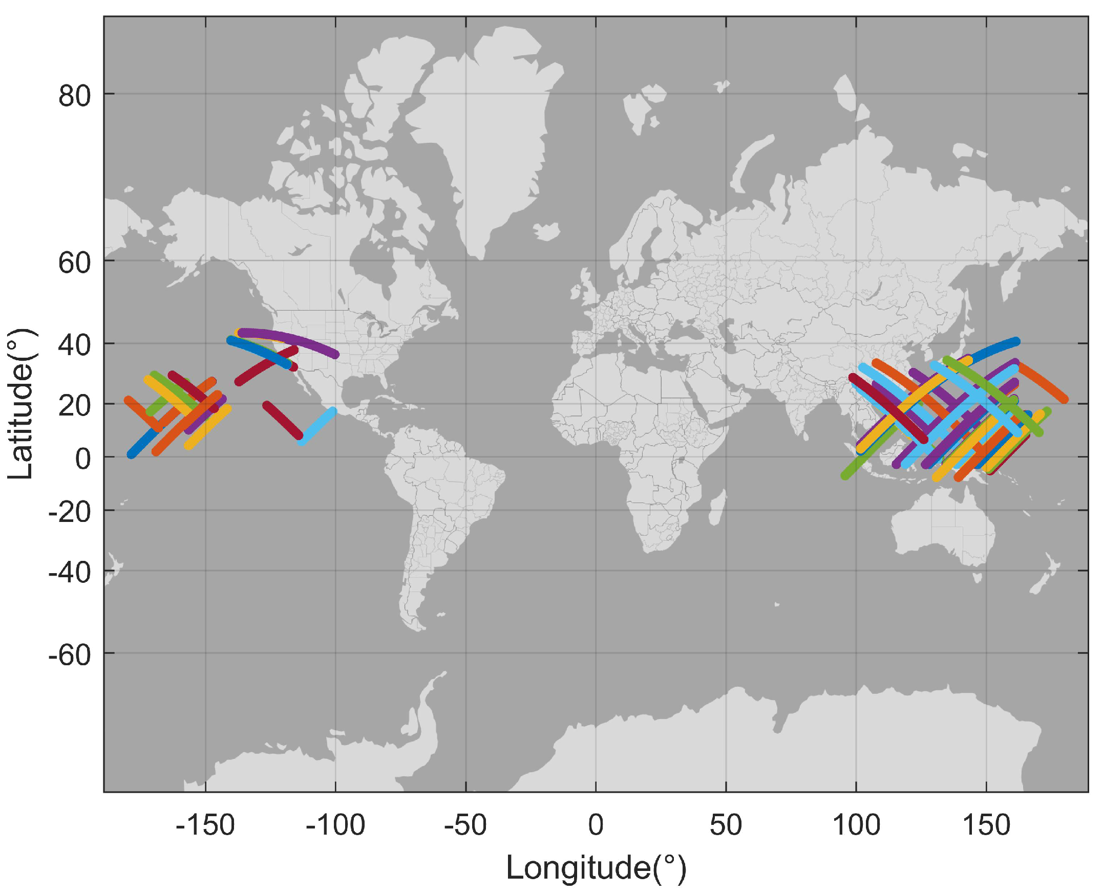
2.1. TG2-InIRA Observations

There are 60 tracks of TG2-InIRA data used in this work as shown in Figure 1, which were taken at intermittent times from December 2016 to February 2019. TG2-InIRA works at incidence angles from 2° to 8° and the ground swath is wider than 30 km at an orbit height of around 400 km. The original σ 0 image resolution in cross-track direction ranges from about 30 m to 200 m, depending on the incidence angle, and the along-track resolution is about 30 m. Figure 2a,b presents one of the SSH images and the corresponding σ 0 image from TG2-InIRA. Preprocessing and quality control are carried out on the data before inputting them into the model. The data contaminated by rainfalls are first screened out before the following processing. Then, ETOPO1 data are used to remove land and nearshore data. Finally, we perform 3 σ filtering on the data to remove the abnormal data. The spatial averaging filtering is performed on original σ 0 images to obtain 5-km-resolution σ 0 as one of the inputs of the model. In addition, the original SSH image resolution in the cross-track direction ranges from about 30 m to 200 m, depending on the incidence angle, and the along-track resolution is about 30 m. In the geocoding processing, the SSH data are resampled into a 30 m grid with 200 m resolution. In our work, we use the SSH image with 200 m resolution. SSH data are another input that contains the high-frequency sea surface features relating to wind and waves.

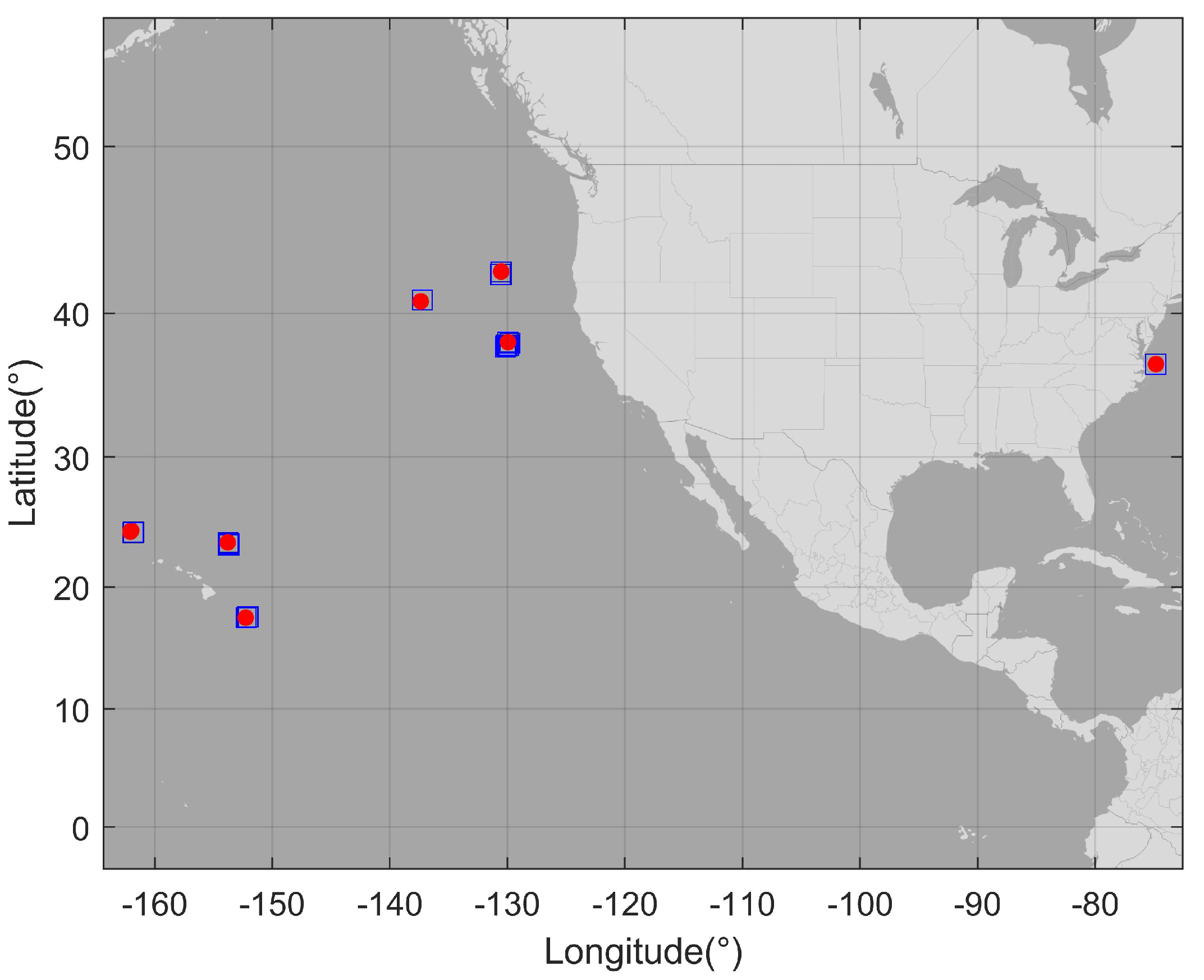
2.2. NDBC Buoys Data

NDBC buoys measure the wind speed directly and the published wind speed data are the ten-minute average wind speed values in m/s. Due to its excellent measurement quality, it has been widely used in the validation of the retrieved results of remote sensing data. The proposed approaches are validated using the wind speeds and SWHs from NDBC buoys (https://www.ndbc.noaa.gov/, accessed on 8 December 2020) 50 km away from offshore. Figure 3 shows the spatial distribution of the collocated buoy data and TG2-InIRA data. There are seven buoys matched to 19 tracks of TG2-InIRA data.
Given that the buoys measure the wind speed every 10 min, a time and spatial matching windows of 10 min and 50 km are used to collocate wind speed. Considering that the measured wind speeds are also about 3–9 m above the sea surface, the wind speed should be transferred to the wind speed at 10 m according to the following equation [43]:
u = 8.7403 × u z l n z 0.0016 ,
where u is the wind speed at 10 m, u z represent the wind speed at z m.
Because the buoys measure the SWH every 10 min or 1 h, the time matching window of 30 min is applied for collocating, which ensures us to get the most appropriately collocated SWH data. The spatial matching window is 50 km.

2.3. ECMWF ERA-5 Data

The collocated reanalysis data are obtained by matching 41 tracks of TG2-InIRA measurements with ECMWF ERA-5 data (https://www.ecmwf.int/en/forecasts/dataset/ecmwf-reanalysis-v5, accessed on 3 January 2021), which provide hourly reanalysis data with atmospheric and ocean-wave quantities. The spatial resolution of a wind speed 10 m above the horizontal is 25 km × 25 km, and the spatial resolution of SWH is 50 km × 50 km, while the temporal resolutions are both 1 h. According to a 10-min time window and 5-km spatial window, a total of 124,258 groups of collocated data are obtained.

2.4. ETOPO1 Data

The ETOPO1 (https://ngdc.noaa.gov/mgg/global/global.html, accessed on 17 August 2020) is a global elevation model that provides elevation data including land topography and ocean bathymetry. The ETOPO1 values between −50 and 0 m are coastal bathymetry [44]. Therefore, ETOPO1 ocean depth data are used to screen out the sea area with water depth less than 50 m to get rid of the coastal effects on the measurements.

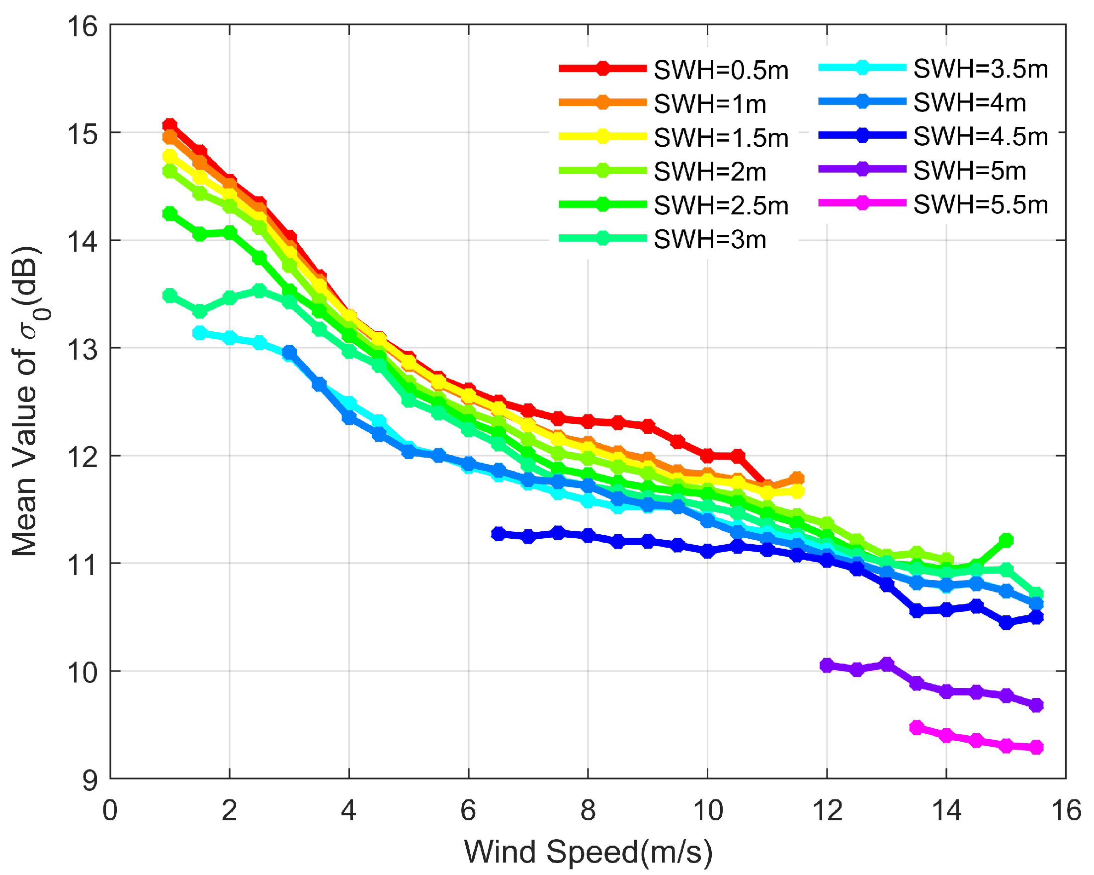
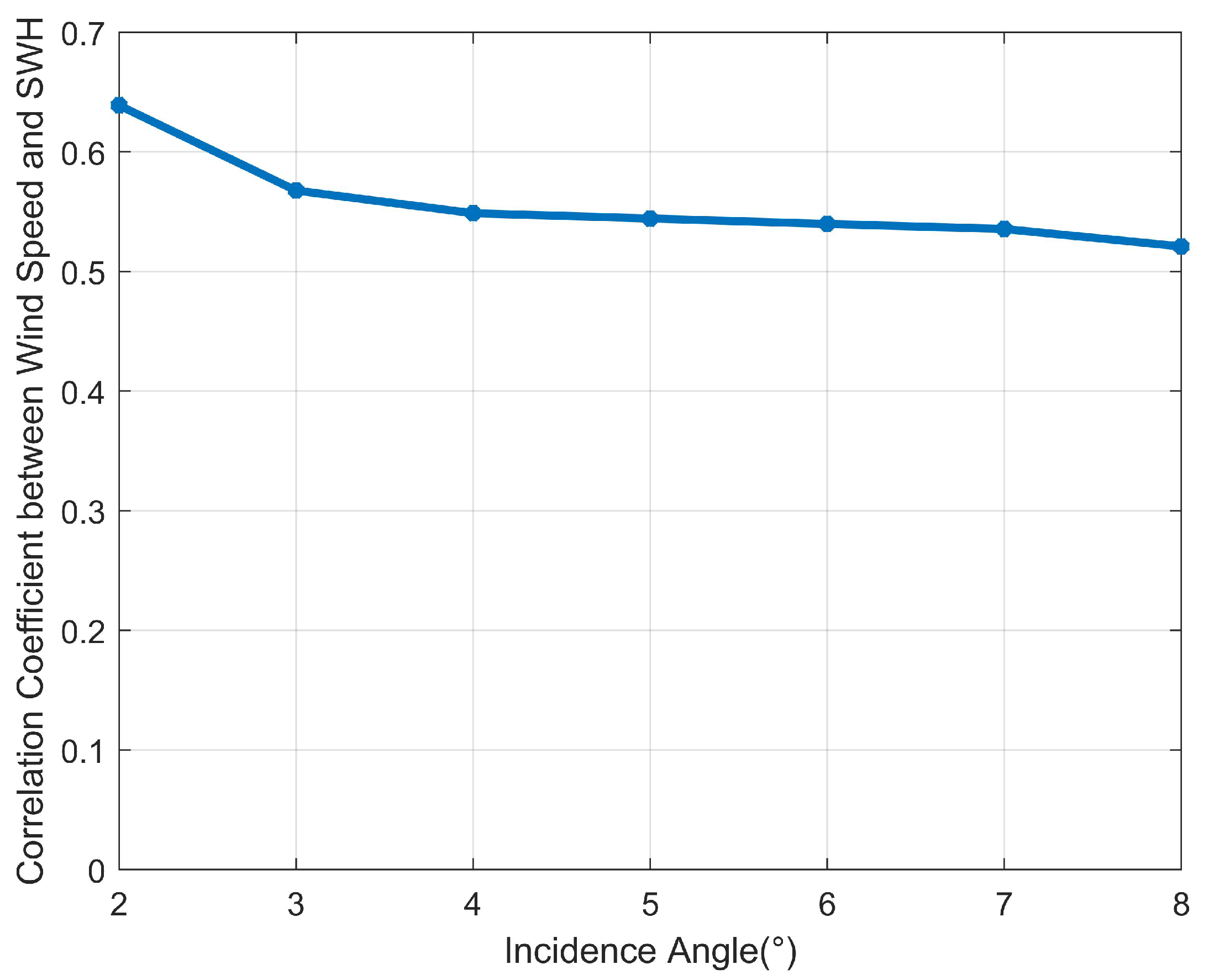
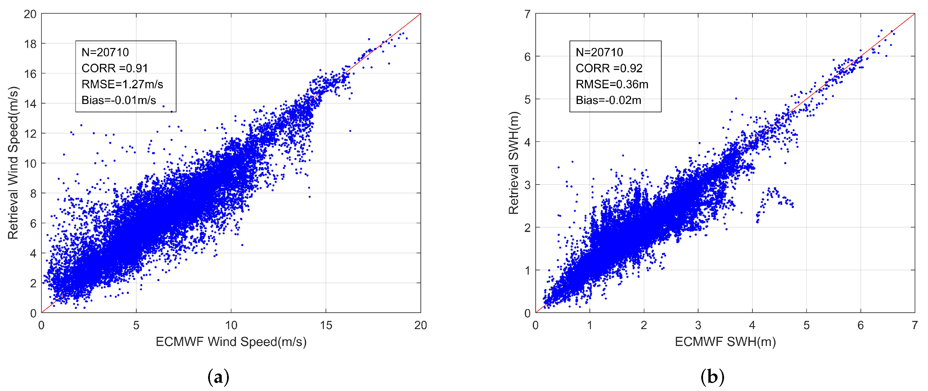
3. Joint Retrieval Model for Wind Speed and SWH

SWH is statistically defined as the mean of the highest 1/3 of the waves, which can be calculated using the standard deviation (STD) of SSH using (4) [34].
S W H = 4 ζ 2 1 2 ,
where ζ is the sea-surface height, and ζ 2 1 2 is the STD of the SSH.
The high-resolution SSH obtained by TG2-InIRA not only contains geoid signal ( h g ), the ocean dynamic topography ( η ), and measurement noise (w) but also includes the high-frequency features of the sea surface which are related to wind speed (u) and SWH [45,46,47]. Consequently, the SSH measured by TG2-InIRA can be expressed as:
S S H T G 2 I n I R A = h g + η + f ( u , S W H ) + w .
As mentioned in Section 1, the correlations among σ 0 , wind speed, and SWH at incidence angles under 20° have been studied extensively based on TRMM PR measurements. The research results in [27] indicated that σ 0 decreases monotonically with increasing wind speed and SWH near nadir. We have received the same results in the analysis of TG2-InIRA, and Figure 4 shows the variations of σ 0 measured by TG2-InIRA under different SWHs and wind speeds at 5° incidence angle for example. It can be seen that σ 0 decreases as SWH increases at the same wind speed and decreases as wind speed increases at the same SWH. Thus, σ 0 can be expressed as a function of u, SWH, and θ :
σ 0 = f ( u , S W H , θ ) .
As shown in (5), the SWH is certainly related to the measurement accuracy of SSH and thus the σ 0 is related to it also. We should point out here that only the relative SSH is enough, it means that the SSH used in this work does not need to be fully calibrated with all kinds of errors corrected as done for traditional altimeters. Because the issue of SSH processing is very complicated and is out of the scope of this work, we only mention here that the relative accuracy of the SSH for TG2-InIRA is about 1–2 m, which corresponds to a spatial resolution of 200 m × 200 m.
In addition, to better explore the relationship between wind speed and SWH, we calculate the Spearman’s rank correlation coefficients between them at different incidence angles, and show the results in Figure 5. The Spearman rank correlation coefficient is a nonparametric measure of statistical dependence between two variables, assessing how well the relationship between two variables can be described using a monotonic function. A correlation coefficient equal to 0.50 indicates a moderate correlation [48]. As can be seen, the correlation coefficients are all greater than 0.5, and they are especially much larger for smaller incidence angles. This means that there is a strong correlation between wind speed and SWH, and the correlation is stronger at smaller angles. Based on the above analysis and observations, the MLP model is developed with σ 0 , SSH, and the incidence angle as the inputs, to be used to jointly retrieve wind speed and SWH. The MLP has a strong generalization ability for nonlinear mapping [41,42], which is a feed-forward and fully connected neural network with one or more layers of nodes between input and output nodes. These in-between layers are called hidden layers.
In our work, 5/6 of the data, i.e., 103,548 groups were randomly selected for model training and the remaining 1/6, i.e., 20,710 groups were used for model testing. Wu et al. [49] retrieved SWH from Sentinel-1 SAR data based on the back-propagation neural network, and the retrieved results show that underestimation enlarges as SWH increases. The reason is that the amount of data in the training dataset in the high sea state is far less than the amount of data in a low to moderate sea state, which roughly follows a Rayleigh distribution. Thus, the training data were adjusted to a normal distribution to effectively solve the underestimation problem. In our work, as shown in Figure 6a, the training SWH data also follows a Rayleigh distribution, which was adjusted to a normal distribution by duplicating and down-sampling according to the mean value and the STD of SWH, as shown in Figure 6b. Besides, as shown in Figure 6c, the distribution of the wind speed training dataset is also close to a normal distribution after reorganization. Moreover, in order to make all input features have the same metric and improve the training efficiency, the inputs are normalized and outputs are de-normalized in the output layer. The objective of the MLP model is to obtain an optimal mapping function that represents the relationship between the input and the output. The back-propagation algorithm was used as the training method to minimize the cost function J ( W , b ) [50], by which the proper learning weights (W) and bia (b) are obtained via computing the discrepancy between the desired and the actual outputs and feeding the error signal level-by-level back to the inputs.
J ( W , b ) = 1 2 i = 1 m y i ^ y i 2 ,
where J ( W , b ) characterizes the deviation between the estimated output y i ^ and the truth y i , m represents the amount of data.
Balancing network performance and training efficiency, different structure realizations (e.g., different number of layers and the different number of neurons in each layer) of MLP were tested by using the training dataset. The training accuracy (result) of the three-layer network is not satisfied. If the five-layer network is used, the accuracy (result) is not significantly improved compared with the four-layer network, but the training efficiency is obviously reduced. In this way, an optimal 4-layer MLP is obtained, and thus the 4-layer joint retrieval model can be constructed as shown in Figure 7, i.e., one input layer for σ 0 , SSH, and the incidence angle, two hidden layers (h1 and h2) with 285 and 87 neurons, respectively, and one output layer for wind speed and SWH. The whole network can be expressed as follows:
h 1 = σ ( W 1 x + b 1 )
h 2 = σ ( W 2 × h 1 + b 2 )
y ^ = W o × h 2 + b o ,
where W and b are the weight and bias of the network. The neurons in the h i   ( i = 1 , 2 ) hidden layer are obtained via pointwise nonlinear mapping of the linearly weighted neurons of the previous layer using function σ ( · ) , where σ ( · ) is the sigmoid function as expressed by (11), which is used in both the input and the hidden layers.
σ ( z ) = 1 1 + e z .
In the retrieval stage, the feature vector x is input to the model, and the best output estimate y ^ is obtained according to Equations (8)–(10). The block diagram of the proposed joint retrieval approach is given in Figure 8, whose major steps have been explained above.
Figure 9 shows the joint retrieval results in comparison with the test set, which is the other 1/6 (20,710 groups) of the collocated ECMWF data. As is shown in Figure 9a, the correlation (CORR) between the retrieved wind speed and the test set is about 0.91 and the RMSE of the retrieved wind speed is about 1.27 m/s with a mean difference (bias) of −0.01 m/s. As is shown in Figure 9b, the CORR between the retrieved SWH and the test set is about 0.92, and the RMSE is about 0.36 m with a bias of −0.02 m. In previous works on TG2-InIRA, 1.85 m/s RMSE of wind speed by using a neural network and 0.43 m RMSE of SWH by using an empirical model have been achieved [38,40]. In [39], a new Ku-band geophysical model function was developed for TG2-InIRA wind speed retrieval and 1.42 m/s RMSE has been achieved. Compared with the previous results, it is shown that more accurate retrievals of both wind speed and SWH are achieved by the proposed joint retrieval method.
Furthermore, it can be seen from the retrieved results shown in Figure 9 that there are relatively more scattered points on the left side of ‘y = x’. The reason is due to a relatively lower amount of training data for lower SWHs and wind speeds, which can be clearly seen in Figure 10a,b. As is shown, the larger the amount of training data, the better the retrieved result, and on the contrary, the lower the amount of training data, the worse the retrieved result, e.g., the regions bounded by the two red rectangles.

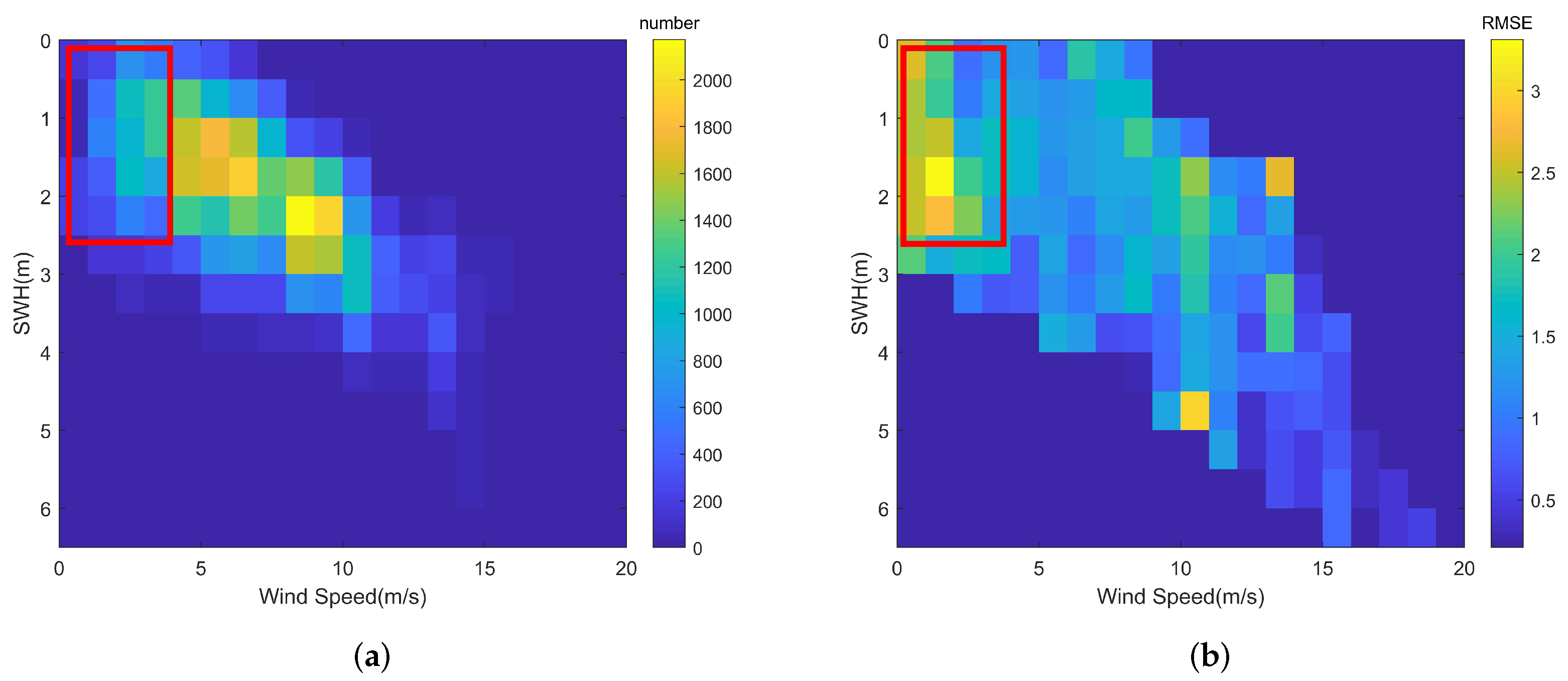
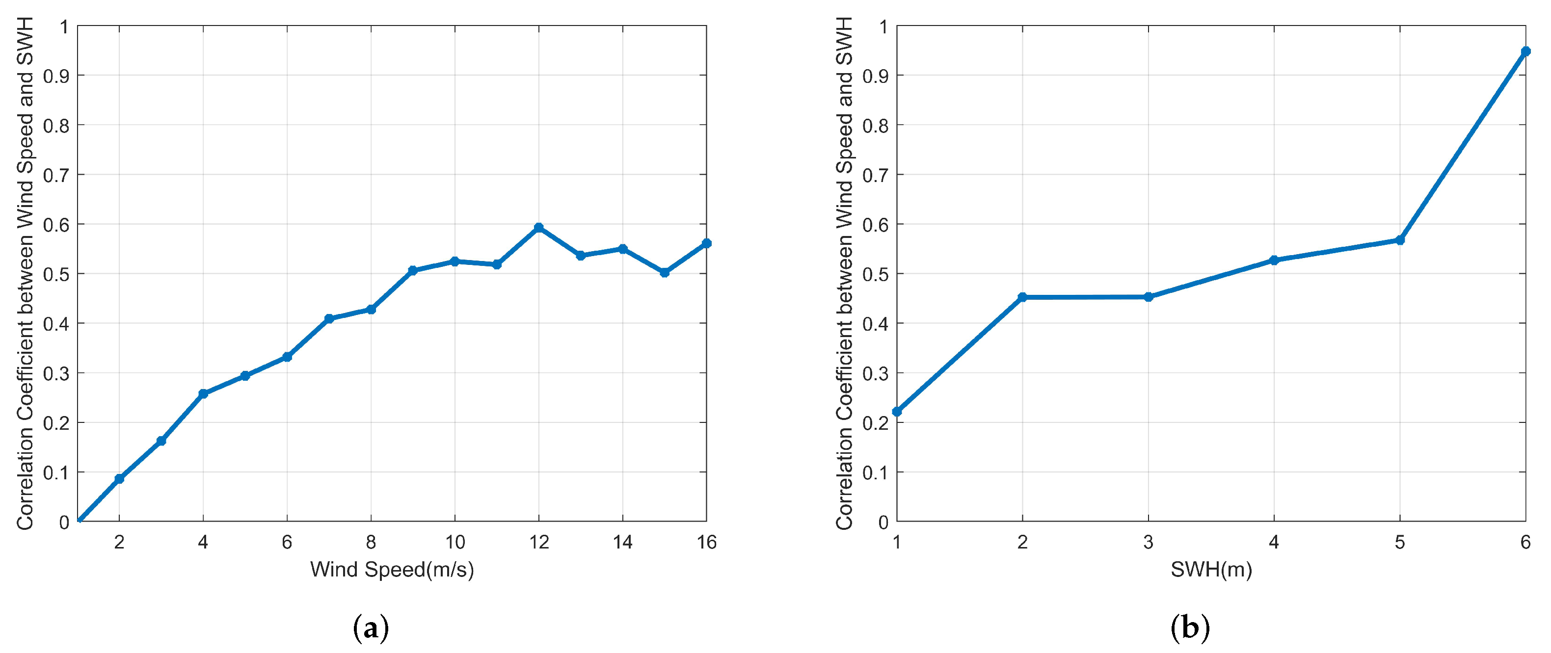
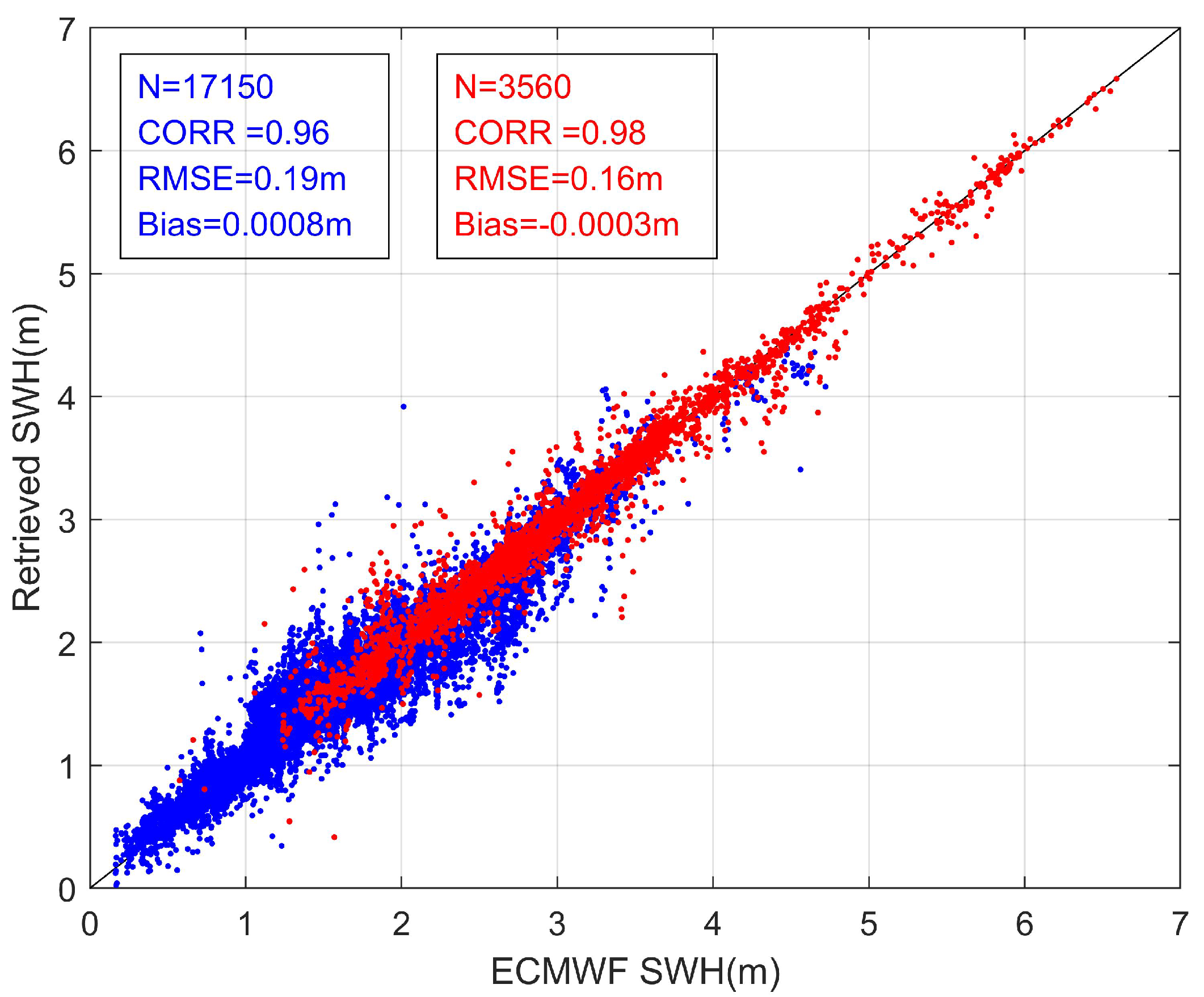
4. Enhanced Joint Retrieval of Wind Speed and SWH

For traditional altimeters, it is concluded that the wind speed retrieval method using SWH information can obtain better results than the method without using SWH information [4]. For InIRA, the previous retrieval of sea surface wind speed did not consider the influence of SWH [37,38,39], or the retrieval of SWH did not consider the influence of wind speed [40]. The above analysis inspires us to make use of the wind speed/SWH information, to further improve the accuracy of SWH/wind speed retrieval for InIRA.
We also use 5/6 of the data for model training and the remaining 1/6 for model testing. In order to ensure the comparability of results, the same neural network structure as Figure 7 is used. For wind speed retrieval, the inputs of the network are σ 0 , SSH, incidence angle, and the retrieved SWH from the proposed joint retrieval model. Figure 11a presents the retrieved wind speed after adding SWH information, and the RMSE is about 1.14 m/s. For SWH retrieval, the inputs of the network are σ 0 , SSH, incidence angle, and the retrieved wind speed from the proposed joint retrieval model. Figure 11b presents the retrieved SWH after adding wind speed information, and the RMSE is about 0.32 m. The result is slightly improved after adding wind speed/SWH information.
In addition, we calculate the Spearman’s rank correlation coefficients between wind speed and SWH at different wind speeds and different SWHs at a 5° incidence angle, and present the results in Figure 12. A correlation coefficient equal to 0.50 indicates a moderate correlation. As can be seen from Figure 12a,b, the correlation coefficients exceed 0.5 when the wind speeds ≥ 9 m/s and the SWHs ≥ 4 m, which means that wind speed and SWH have a stronger relationship under higher wind speed and larger SWH scenarios, and thus the influence of SWH on wind speed retrieval should not be neglected, and vice versa. Therefore, we further explore the influence of different correlations between them on the retrieved results. The block diagram of the enhanced method is presented in Figure 13, as it is shown that both the wind speed and the SWH are divided into two regions and the enhanced models are developed accordingly.
It is well known that SWH can be used to characterize the sea state, which has been justified by the collocated SWH data obtained directly from altimeters. Low SWHs represent young sea, whereas high SWHs are associated mostly with mixed seas including swells [51]. When SWH is ≥ 4 m, the correlation coefficients between wind speed and SWH are larger than 0.5. Therefore, based on the jointly retrieved SWH, we establish the enhanced wind speed retrieval models for higher sea state and lower sea state, respectively, with SWH of 4 m as the distinguishing criterion. Thus, the data are firstly divided into two regions, i.e., SWHs < 4 m and SWHs ≥ 4 m, and then the wind speed retrieval models are established for different SWH regions. The training data set is still 5/6 of the total, and the test set is the remaining 1/6. The inputs of the enhanced network are σ 0 , SSH, incidence angle, and the retrieved SWH from the proposed joint retrieval model.
The further improved wind speed results are presented in Figure 14, as can be seen, the RMSEs of wind speed corresponding to SWHs < 4 m and SWHs ≥ 4 m regions are respectively about 1.12 m/s and 0.73 m/s. Table 1 summarizes the RMSEs of different wind speed models for clear comparison. By comparing Figure 11a with Figure 14, it is shown that the improvement of wind speed retrieval accuracy for a larger SWH region is better than that for a smaller SWH region because the correlation between wind speed and SWH is much larger for larger SWH than that for smaller SWH.
Similarly, according to the fact that the correlation coefficients between wind speed and SWH are relatively larger for wind speeds ≥ 9 m/s, based on the jointly retrieved wind speed, we develop the enhanced SWH retrieval models for different wind speed regions, respectively, and present the retrieved results in Figure 15. The RMSE for wind speeds < 9 m/s is about 0.19 m, while it is about 0.16 m for wind speeds ≥ 9 m/s. The RMSE results are summarized in Table 2. As before, the larger the correlation, the greater the improvement of SWH results.
It is also demonstrated that the further improved performances on SWH by the enhanced models are relatively better than that on wind speed by the enhanced models as easily seen if comparing Figure 14 and Figure 15 or comparing Table 1 and Table 2. The correlation coefficients corresponding to different SWHs are larger than those of different wind speeds on the whole, as shown in Figure 12.

5. Validated by Buoy and Discussion

In this section, we further validate the derived approaches by comparing the retrieved wind speeds and SWHs with those from buoys. Because the TG2-InIRA’s daily observation time is limited to 15–20 min, the covered buoys are quite limited. Only seven NDBC buoys are collocated with TG2-InIRA data, and a total of 19 groups of collocated data are obtained. We compare the wind speeds and SWHs retrieved from the joint retrieval model, the enhanced models, and the collocated buoys. It is clearly shown in Figure 16 that the retrieved results are all highly consistent with the buoy data, except for the third group with extraordinarily large errors presented and the reason is that the available measurements as depicted in the red rectangle in Figure 17 for wind speeds around 13.57 m/s and SWH around 3.25 m are much less than others and thus the model is not sufficiently trained.
In the following, the joint retrieval results and the enhanced retrieval results are compared with the buoy data in detail. The enhanced retrievals are overall better than the joint retrievals and the wind speed RMSE is 0.88 m/s and the SWH RMSE is 0.36 m, while they are respectively 1.41 m/s and 0.50 m (without including the No.3 group) for the joint retrieval. As it is shown in Figure 16, for 13 of the total 19 groups, the enhanced retrievals of both wind speed and SWH are better than the joint retrievals, while for the remaining six groups (No.2, 4, 8, 11, 14, 15), or the wind speeds or the SWHs of the enhanced retrieval are better than the joint retrievals and specifically if the enhanced wind speed or SWH is much better than the joint retrieval, then the enhanced SWH or wind speed is not better. This phenomenon happens when the jointly retrieved wind speed/SWH is already of higher accuracy, so the enhanced SWH/wind speed can be further improved because the wind speed/SWH is taken as the input to the enhanced model, but the cost is to have the accuracy of wind speed/SWH degraded. However, although currently the enhanced retrievals are not always better than the joint retrievals and this is attributed to the reason of less training data of models; it is not true for the future operational missions because plenty of observations under almost all kinds of ocean conditions can be accumulated to train the models.

6. Conclusions

The observation mechanism of TG2-InIRA enables it to obtain the measurements of wide-swath SSH and σ 0 with high spatial resolution at the same time. Based on the measurements of TG2-InIRA, a joint retrieval model of wind speed and SWH is developed using MLP, by which simultaneous retrievals of wind speed and SWH are obtained. Besides, the retrieving accuracy of wind speed can be further improved by using SWH information and establishing enhanced wind speed models for different SWH regions. The retrieving accuracy of SWH can also be improved by establishing the enhanced SWH models for different wind speeds. In addition, the higher the correlation, the greater the improvement of the enhanced model.
This work demonstrates that the correlation between the wind speed and the SWH at small incidence angles can be used to retrieve them simultaneously; furthermore, the additional information of SWH can be utilized to improve the wind speed retrieval accuracy, or the additional information of wind speed can be utilized to improve the accuracy of SWH retrieval significantly. In addition, in the current work, the method for rainfall detection is not automatic and is less efficient. In our future work, on one hand, a more efficient method should be adopted for rainfall detection, e.g., those in [52,53], and on the other hand, the rain contaminated image can be used to retrieve training.

Author Contributions

Conceptualization, G.L., Y.Z. and X.D.; methodology, G.L. and X.D.; validation, G.L.; writing—original draft preparation, G.L.; writing—revising and editing, G.L., Y.Z. and X.D. All authors have read and agreed to the published version of the manuscript.

Funding

This research was funded by the National Key R&D Program of China under Grant 2016YFC1401004, along with China Manned Space Program.

Institutional Review Board Statement

Not applicable.

Informed Consent Statement

Not applicable.

Data Availability Statement

The TG2-InIRA data are from National Satellite Ocean Application Service and are copied by disk. The NDBC buoy data are from (https://www.ndbc.noaa.gov/, accessed on 8 December 2020). The ETOPO1 digital elevation model data are from NOAA’s National Centers for Environmental Information (https://ngdc.noaa.gov/mgg/global/global.html, accessed on 17 August 2020). The ERA5 data are from European Centre for Medium-Range Weather Forecasts (https://www.ecmwf.int/en/forecasts/dataset/ecmwf-reanalysis-v5, accessed on 3 January 2021).

Acknowledgments

The authors would like to thank the European Centre for Medium-Range Weather Forecasts for the straightforward and rapid electronic access to the ERA-5 reanalysis data. The authors would also like to thank the American National Data Buoy Center for providing the buoy data and the NOAA’s National Centers for Environmental Information for providing the ETOPO1 data.

Conflicts of Interest

The authors declare no conflict of interest.

References

  1. Horstmann, J.; Schiller, H.; Schulz-Stellenfleth, J.; Lehner, S. Global Wind Speed Retrieval from Sar. IEEE Trans. Geosci. Remote Sens. 2003, 41, 2277–2286. [Google Scholar] [CrossRef] [Green Version]
  2. Witter, D.L.; Chelton, D.B. A Geosat Altimeter Wind Speed Algorithm and a Method for Altimeter Wind Speed Algorithm Development. J. Geophys. Res. 1991, 96, 8853–8860. [Google Scholar] [CrossRef]
  3. Monaldo, F.; Thompson, D.; Pichel, W.; Clemente-Colon, P. A Systematic Comparison of QuikSCAT and SAR Ocean Surface Wind Speeds. IEEE Trans. Geosci. Remote Sens. 2004, 42, 283–291. [Google Scholar] [CrossRef]
  4. Brown, G.; Stanley, H.; Roy, N. The Wind-Speed Measurement Capability of Spaceborne Radar Altimeters. IEEE J. Ocean. Eng. 1981, 6, 59–63. [Google Scholar] [CrossRef]
  5. Chelton, D.B.; McCabe, P.J. A Review of Satellite Altimeter Measurement of Sea Surface Wind Speed: With a Proposed New Algorithm. J. Geophys. Res. 1985, 90, 4707–4720. [Google Scholar] [CrossRef]
  6. Monaldo, F.; Dobson, E. On Using Significant Wave Height and Radar Cross Section to Improve Radar Altimeter Measurements of Wind Speed. J. Geophys. Res. 1989, 94, 12699–12701. [Google Scholar] [CrossRef]
  7. Lefevre, J.M.; Barckicke, J.; Ménard, Y. A Significant Wave Height Dependent Function for TOPEX/POSEIDON Wind Speed Retrieval. J. Geophys. Res. 1994, 99, 25035–25049. [Google Scholar] [CrossRef]
  8. Hasselmann, K.; Hasselmann, S. On the Nonlinear Mapping of an Ocean Wave Spectrum into a Synthetic Aperture Radar Image Spectrum and Its Inversion. J. Geophys. Res. 1991, 96, 10713–10729. [Google Scholar] [CrossRef]
  9. Engen, G.; Johnsen, H. SAR-ocean Wave Inversion Using Image Cross Spectra. IEEE Trans. Geosci. Remote Sens. 1995, 33, 1047–1056. [Google Scholar] [CrossRef]
  10. Li, X.; Lehner, S.; Bruns, T. Ocean Wave Integral Parameter Measurements Using Envisat ASAR Wave Mode Data. IEEE Trans. Geosci. Remote Sens. 2011, 49, 155–174. [Google Scholar] [CrossRef] [Green Version]
  11. Schulz-Stellenfleth, J.; Konig, T.; Lehner, S. An Empirical Approach for the Retrieval of Ocean Wave Parameters from Synthetic Aperture Radar Data. In Proceedings of the 2006 IEEE International Symposium on Geoscience and Remote Sensing, Denver, CO, USA, 31 July–4 August 2006; pp. 1875–1878. [Google Scholar] [CrossRef]
  12. Stopa, J.E.; Mouche, A. Significant Wave Heights from Sentinel-1 SAR: Validation and Applications: EMPIRICAL WAVE PARAMETERS FOR SENTINEL-1. J. Geophys. Res. Oceans 2017, 122, 1827–1848. [Google Scholar] [CrossRef] [Green Version]
  13. Yang, X.; Li, X.; Pichel, W.G.; Li, Z. Comparison of Ocean Surface Winds From ENVISAT ASAR, MetOp ASCAT Scatterometer, Buoy Measurements, and NOGAPS Model. IEEE Trans. Geosci. Remote Sens. 2011, 49, 4743–4750. [Google Scholar] [CrossRef]
  14. Zhang, B.; Mouche, A.; Lu, Y.; Perrie, W.; Zhang, G.; Wang, H. A Geophysical Model Function for Wind Speed Retrieval From C-Band HH-Polarized Synthetic Aperture Radar. IEEE Geosci. Remote Sens. Lett. 2019, 16, 1521–1525. [Google Scholar] [CrossRef]
  15. Apel, J.R. An Improved Model of the Ocean Surface Wave Vector Spectrum and Its Effects on Radar Backscatter. J. Geophys. Res. 1994, 99, 16269–16291. [Google Scholar] [CrossRef]
  16. Romeiser, R.; Alpers, W. An Improved Composite Surface Model for the Radar Backscattering Cross Section of the Ocean Surface: 2. Model Response to Surface Roughness Variations and the Radar Imaging of Underwater Bottom Topography. J. Geophys. Res. Oceans 1997, 102, 25251–25267. [Google Scholar] [CrossRef]
  17. Chen, K.; Fung, A.; Weissman, D. A Backscattering Model for Ocean Surface. IEEE Trans. Geosci. Remote Sens. 1992, 30, 811–817. [Google Scholar] [CrossRef]
  18. Stoffelen, A.; Anderson, D. Scatterometer Data Interpretation: Estimation and Validation of the Transfer Function CMOD4. J. Geophys. Res. Oceans 1997, 102, 5767–5780. [Google Scholar] [CrossRef]
  19. Portabella, M. Toward an Optimal Inversion Method for Synthetic Aperture Radar Wind Retrieval. J. Geophys. Res. 2002, 107, 3086. [Google Scholar] [CrossRef]
  20. Xie, X.; Chen, K.; Yu, W.; Hu, W.; Zeng, Q.; Fang, Y. A Study on Geophysical Model Function Modeling with Water Surface Temperature as One of the Input Parameters. In Proceedings of the IGARSS 2008—2008 IEEE International Geoscience and Remote Sensing Symposium, Boston, MA, USA, 6–11 July 2008; Volume 1, pp. I-398–I-401. [Google Scholar] [CrossRef]
  21. Stiles, B.W.; Danielson, R.E.; Poulsen, W.L.; Brennan, M.J.; Hristova-Veleva, S.; Shen, T.P.; Fore, A.G. Optimized Tropical Cyclone Winds From QuikSCAT: A Neural Network Approach. IEEE Trans. Geosci. Remote Sens. 2014, 52, 7418–7434. [Google Scholar] [CrossRef]
  22. Liu, Y.; Collett, I.; Morton, Y.J. Application of Neural Network to GNSS-R Wind Speed Retrieval. IEEE Trans. Geosci. Remote Sens. 2019, 57, 9756–9766. [Google Scholar] [CrossRef]
  23. Thiria, S.; Mejia, C.; Badran, F.; Crepon, M. A Neural Network Approach for Modeling Nonlinear Transfer Functions: Application for Wind Retrieval from Spaceborne Scatterometer Data. J. Geophys. Res. 1993, 98, 22827–22841. [Google Scholar] [CrossRef]
  24. Kumar, N.K.; Savitha, R.; Al Mamun, A. Ocean Wave Height Prediction Using Ensemble of Extreme Learning Machine. Neurocomputing 2018, 277, 12–20. [Google Scholar] [CrossRef]
  25. Gao, D.; Liu, Y.; Meng, J.; Jia, Y.; Fan, C. Estimating Significant Wave Height from SAR Imagery Based on an SVM Regression Model. Acta Oceanol. Sin. 2018, 37, 103–110. [Google Scholar] [CrossRef]
  26. Xue, S.; Geng, X.; Yan, X.H.; Xie, T.; Yu, Q. Significant Wave Height Retrieval from Sentinel-1 SAR Imagery by Convolutional Neural Network. J. Oceanogr. 2020, 76, 465–477. [Google Scholar] [CrossRef]
  27. Chu, X.; He, Y.; Karaev, V.Y. Relationships Between Ku-Band Radar Backscatter and Integrated Wind and Wave Parameters at Low Incidence Angles. IEEE Trans. Geosci. Remote Sens. 2012, 50, 4599–4609. [Google Scholar] [CrossRef]
  28. Yan, Q.; Zhang, J.; Fan, C.; Meng, J. Analysis of Ku- and Ka-Band Sea Surface Backscattering Characteristics at Low-Incidence Angles Based on the GPM Dual-Frequency Precipitation Radar Measurements. Remote Sens. 2019, 11, 754. [Google Scholar] [CrossRef] [Green Version]
  29. Karaev, V.Y.; Kanevsky, M.B.; Balandina, G.N.; Cotton, P.D.; Challenor, P.G.; Gommenginger, C.P.; Srokosz, M.A. On the Problem of the near Ocean Surface Wind Speed Retrieval by Radar Altimeter: A Two-Parameter Algorithm. Int. J. Remote Sens. 2002, 23, 3263–3283. [Google Scholar] [CrossRef]
  30. Gourrion, J.; Vandemark, D.; Bailey, S.; Chapron, B.; Gommenginger, G.P.; Challenor, P.G.; Srokosz, M.A. A Two-Parameter Wind Speed Algorithm for Ku-Band Altimeters. J. Atmos. Ocean. Technol. 2002, 19, 2030–2048. [Google Scholar] [CrossRef]
  31. Glazman, R.E.; Greysukh, A. Satellite Altimeter Measurements of Surface Wind. J. Geophys. Res. Oceans 1993, 98, 2475–2483. [Google Scholar] [CrossRef]
  32. Jiang, H.; Zheng, H.; Mu, L. Improving Altimeter Wind Speed Retrievals Using Ocean Wave Parameters. IEEE J. Sel. Top. Appl. Earth Obs. Remote Sens. 2020, 13, 1917–1924. [Google Scholar] [CrossRef]
  33. Webster, P.J.; Moore, A.M.; Loschnigg, J.P.; Leben, R.R. Coupled Ocean–Atmosphere Dynamics in the Indian Ocean during 1997–98. Nature 1999, 401, 356–360. [Google Scholar] [CrossRef]
  34. Stewart, R.H. Introduction to Physical Oceanography; Prentice-Hall: Upper Saddle River, NJ, USA, 2008. [Google Scholar]
  35. Dong, X.; Zhang, Y.; Zhai, W. Design and Algorithms of the Tiangong-2 Interferometric Imaging Radar Altimeter Processor. In Proceedings of the 2017 Progress in Electromagnetics Research Symposium-Spring (PIERS), St. Petersburg, Russia, 22–25 May 2017; pp. 3802–3803. [Google Scholar] [CrossRef]
  36. Zhang, Y.; Shi, X.; Wang, H.; Tan, Y.; Zhai, W.; Dong, X.; Kang, X.; Yang, Q.; Li, D.; Jiang, J. Interferometric Imaging Radar Altimeter on Board Chinese Tiangong-2 Space Laboratory. In Proceedings of the 2018 Asia-Pacific Microwave Conference (APMC), Kyoto, Japan, 6–9 November 2018; pp. 851–853. [Google Scholar] [CrossRef]
  37. Ren, L.; Yang, J.; Jia, Y.; Dong, X.; Wang, J.; Zheng, G. Sea Surface Wind Speed Retrieval and Validation of the Interferometric Imaging Radar Altimeter Aboard the Chinese Tiangong-2 Space Laboratory. IEEE J. Sel. Top. Appl. Earth Obs. Remote Sens. 2018, 11, 4718–4724. [Google Scholar] [CrossRef]
  38. Zhang, Y.; Bao, Q.; Lin, M.; Lang, S. Wind Speed Inversion and In-Orbit Assessment of the Imaging Altimeter on Tiangong-2 Space Station. Acta Oceanol. Sin. 2020, 39, 114–120. [Google Scholar] [CrossRef]
  39. Li, G.; Zhang, Y.; Dong, X. New Ku-Band Geophysical Model Function and Wind Speed Retrieval Algorithm Developed for Tiangong-2 Interferometric Imaging Radar Altimeter. IEEE J. Sel. Top. Appl. Earth Obs. Remote Sens. 2022, 15, 1981–1991. [Google Scholar] [CrossRef]
  40. Ren, L.; Yang, J.; Dong, X.; Jia, Y.; Zhang, Y. Preliminary Significant Wave Height Retrieval from Interferometric Imaging Radar Altimeter Aboard the Chinese Tiangong-2 Space Laboratory. Remote Sens. 2021, 13, 2413. [Google Scholar] [CrossRef]
  41. Khotanzad, A.; Lu, J.H. Distortion Invariant Character Recognition by a Multi-Layer Perceptron and Back-Propagation Learning. In Proceedings of the IEEE 1988 International Conference on Neural Networks, San Diego, CA, USA, 24–27 July 1988; Volume 1, pp. 625–632. [Google Scholar] [CrossRef]
  42. Pal, S.; Mitra, S. Multilayer Perceptron, Fuzzy Sets, and Classification. IEEE Trans. Neural Netw. 1992, 3, 683–697. [Google Scholar] [CrossRef]
  43. Thomas, B.R.; Kent, E.C.; Swail, V.R. Methods to Homogenize Wind Speeds from Ships and Buoys. Int. J. Climatol. 2005, 25, 979–995. [Google Scholar] [CrossRef]
  44. Amante, C. ETOPO1 1 Arc-Minute Global Relief Model: Procedures, Data Sources and Analysis; National Geophysical Data Center, NOAA: Washington, DC, USA, 2009. [CrossRef]
  45. Gaspar, P.; Florens, J.P. Estimation of the Sea State Bias in Radar Altimeter Measurements of Sea Level: Results from a New Nonparametric Method. J. Geophys. Res. Oceans 1998, 103, 15803–15814. [Google Scholar] [CrossRef]
  46. Andersen, O.B. Marine Gravity and Geoid from Satellite Altimetry. In Geoid Determination; Sansò, F., Sideris, M.G., Eds.; Springer: Berlin/Heidelberg, Germnay, 2013; Volume 110, pp. 401–451. [Google Scholar] [CrossRef]
  47. Chelton, D.B. The Sea State Bias in Altimeter Estimates of Sea Level from Collinear Analysis of TOPEX Data. J. Geophys. Res. 1994, 99, 24995. [Google Scholar] [CrossRef]
  48. Fowler, J.; Cohen, L.; Jarvis, P. Practical Statistics for Field Biology; Wiley: Hoboken, NJ, USA, 1998. [Google Scholar]
  49. Wu, K.; Li, X.M.; Huang, B. Retrieval of Ocean Wave Heights From Spaceborne SAR in the Arctic Ocean With a Neural Network. J. Geophys. Res. Oceans 2021, 126, e2020JC016946. [Google Scholar] [CrossRef]
  50. Rumelhart, D.E.; Hinton, G.E.; Williams, R.J. Learning Representations by Back Propagating Errors. Nature 1986, 323, 533–536. [Google Scholar] [CrossRef]
  51. Tran, N.; Chapron, B.; Vandemark, D. Effect of Long Waves on Ku-Band Ocean Radar Backscatter at Low Incidence Angles Using TRMM and Altimeter Data. IEEE Geosci. Remote Sens. Lett. 2007, 4, 542–546. [Google Scholar] [CrossRef] [Green Version]
  52. Zheng, Y.; Shi, Z.; Lu, Z.; Ma, W. A Method for Detecting Rainfall From X-Band Marine Radar Images. IEEE Access 2020, 8, 19046–19057. [Google Scholar] [CrossRef]
  53. Chen, X.; Huang, W.; Zhao, C.; Tian, Y. Rain Detection From X-Band Marine Radar Images: A Support Vector Machine-Based Approach. IEEE Trans. Geosci. Remote Sens. 2020, 58, 2115–2123. [Google Scholar] [CrossRef]
Figure 1. Sixty tracks of TG2-InIRA data used in this study.
Remotesensing 14 01930 g001
Figure 2. Ocean observation images of TG2-InIRA. (a) SSH; (b) σ 0 .
Remotesensing 14 01930 g002
Figure 3. Distribution of NDBC buoys matching to TG2-InIRA. The red points denote the positions of the buoys while the blue squares represent the positions of the collocated TG2-InIRA data.
Remotesensing 14 01930 g003
Figure 4. Mean values of σ 0 at different wind speeds and SWHs at 5° incidence angle. Different colored curves represent different SWH ranges.
Remotesensing 14 01930 g004
Figure 5. Correlation coefficients between wind speed and SWH at different incidence angles.
Remotesensing 14 01930 g005
Figure 6. Histograms of the collocated data for training. (a) original SWH; (b) re-sampled SWH; (c) re-sampled wind speed.
Remotesensing 14 01930 g006
Figure 7. Structure of the four-layer MLP model with one input layer, one output layer and two hidden layers.
Remotesensing 14 01930 g007
Figure 8. Block diagram of the proposed joint retrieval approach.
Remotesensing 14 01930 g008
Figure 9. Joint retrieval results compared with ECMWF reanalysis data. (a) wind speed; (b) SWH. The red line represents the reference line ’y = x’.
Remotesensing 14 01930 g009
Figure 10. Wind speed–SWH distribution. (a)the training data set number, (b) Wind speed–SWH distribution of the RMSE of the retrieved result (wind speed+SWH).
Remotesensing 14 01930 g010
Figure 11. Retrieved results. (a) retrieved wind speed after adding SWH. (b) retrieved SWH after adding wind speed. The black lines are ‘y = x’ for references.
Remotesensing 14 01930 g011
Figure 12. Spearman’s rank correlation coefficients between wind speed and SWH at 5° incidence angle. (a) at different wind speeds; (b) at different SWHs.
Remotesensing 14 01930 g012
Figure 13. Block diagram of the enhanced joint retrieval method.
Remotesensing 14 01930 g013
Figure 14. Retrieved wind speeds by the enhanced model with SWH divided into SWHs < 4 m (blue color) and SWHs ≥ 4 m (red color) regions. The black line is ‘y = x’ for reference.
Remotesensing 14 01930 g014
Figure 15. Retrieved SWHs by enhanced model with wind speed divided into wind speeds < 9 m/s (blue color) and wind speeds ≥ 9 m/s (red color) regions.The black line is ‘y = x’ for reference.
Remotesensing 14 01930 g015
Figure 16. Comparison of the retrieved results and buoys’ data. (a) comparison of the joint retrieved wind speeds, enhanced wind speeds and buoy wind speeds; (b) difference between joint retrieved wind speeds and buoy, and enhanced retrieved wind speeds and buoy; (c) comparison of the joint retrieved SWHs, enhanced SWHs and buoy SWHs; (d) difference between joint retrieved SWHs and buoy, and enhanced retrieved SWHs and buoy.
Remotesensing 14 01930 g016
Figure 17. Wind speed–SWH distribution of the training data set.
Remotesensing 14 01930 g017
Table 1. RMSE of the retrieved wind speed.
ModelWhole DatasetDataset for Low Sea State (SWHs < 4.0 m)Dataset for High Sea State (SWHs ≥ 4.0 m)
Enhanced Wind Speed Model-1.12 m/s0.73 m/s
Model without Data Division1.14 m/s--
Table 2. RMSE of the retrieved SWH.
ModelWhole DatasetDataset for Wind Speeds < 9 m/sDataset for Wind Speeds ≥ 9 m/s
Enhanced SWH Model-0.19 m0.16 m
Model without Data Division0.32 m--
Publisher’s Note: MDPI stays neutral with regard to jurisdictional claims in published maps and institutional affiliations.

