Article

Estimating Hourly Surface Solar Irradiance from GK2A/AMI Data Using Machine Learning Approach around Korea

National Meteorological Satellite Center, Korea Meteorological Administration, Jincheon 27803, Korea
*
Author to whom correspondence should be addressed.
Remote Sens. 2022, 14(8), 1840; https://doi.org/10.3390/rs14081840
Submission received: 28 February 2022 / Revised: 6 April 2022 / Accepted: 7 April 2022 / Published: 11 April 2022
(This article belongs to the Special Issue New Challenges in Solar Radiation, Modeling and Remote Sensing)

Abstract

:
Surface solar irradiance (SSI) is a crucial component in climatological and agricultural applications. Because the use of renewable energy is crucial, the importance of SSI has increased. In situ measurements are often used to investigate SSI; however, their availability is limited in spatial coverage. To precisely estimate the distribution of SSI with fine spatiotemporal resolutions, we used the GEOstationary Korea Multi-Purpose SATellite 2A (GEO-KOMPSAT 2A, GK2A) equipped with the Advanced Meteorological Imager (AMI). To obtain an optimal model for estimating hourly SSI around Korea using GK2A/AMI, the convolutional neural network (CNN) model as a machine learning (ML) technique was applied. Through statistical verification, CNN showed a high accuracy, with a root mean square error (RMSE) of 0.180 MJ m−2, a bias of −0.007 MJ m−2, and a Pearson’s R of 0.982. The SSI obtained through a ML approach showed an accuracy higher than the GK2A/AMI operational SSI product. The CNN SSI was evaluated by comparing it with the in situ SSI from the Ieodo Ocean Research Station and from flux towers over land; these in situ SSI values were not used for training the model. We investigated the error characteristics of the CNN SSI regarding environmental conditions including local time, solar zenith angle, in situ visibility, and in situ cloud amount. Furthermore, monthly and annual mean daily SSI were calculated for the period from 1 January 2020 to 31 January 2022, and regional characteristics of SSI around Korea were analyzed. This study addressed the availability of satellite-derived SSI to resolve the limitations of in situ measurements. This could play a principal role in climatological and renewable energy applications.

Graphical Abstract

1. Introduction

Shortwave radiation emitted from the sun is a primary variable in the Earth’s energy system. Shortwave radiation is a principal driving parameter of atmospheric phenomena including air–land interactions, heat transfer, and gas exchange. As climate change progresses, the precise quantification of surface solar irradiance (SSI) is being emphasized, and SSI is being used in solar energy applications [1]. Furthermore, measurements of SSI, which is considered among the most essential climate variables, have been developed and provided from diverse datasets including the National Centers for Environmental Prediction and the National Center for Atmospheric Research (NCEP/NCAR) reanalysis data, the European Center for Medium Range Weather Forecasts (ECMWF) ERA reanalysis data, Clouds and the Earth’s Radiant Energy System (CERES), the University of Maryland/MODIS (UMD/MODIS), the Climate Monitoring Satellite Application Facility (CM-SAF), and Global Land Surface Satellite (GLASS) products [2,3,4,5,6].
SSI is an important parameter in climatology and agriculture. It was reported that surface radiation was closely related to the canopy response and the normalized difference vegetation index, which is a satellite-derived parameter examining vegetation activity [7,8]. For agricultural application, the gross primary production was estimated based on the satellite-derived radiation products in previous studies [9,10]. Roundy et al. [11] investigated the effects of land–atmospheric coupling on drought prediction. In particular, the fluctuation of SSI has intensified with climate change, and the trends of changes in SSI are region-dependent. Thus, the importance of SSI has been emphasized in agricultural and climatological applications.
Because SSI is affected by the absorption and scattering of aerosols and atmospheric molecules, it has fluctuated with progressing climate change [12]. In addition, precise information on SSI is essential for many climatological and agricultural applications, and it is a vital parameter for designing solar power systems and smart cities. Photovoltaic power, a renewable energy source that is an alternative to fossil fuels, could help tackle climate change. SSI directly affects climate change; hence, the importance of information on SSI is rapidly increasing over time [13]. The energy consumption in Asian countries constitutes over 40% of global energy consumption, and the energy consumption in China, India, Japan, and Korea accounts for over 70% of the energy consumption in Asian countries [14]. These Asian countries usually lack domestic fossil fuels and largely depend on imported fossil fuels; this trend is especially pronounced in Korea [15]. Interest in renewable energy has been increasing as a way to mitigate climate change in Korea; therefore, it is necessary to monitor and analyze SSI with a high degree of accuracy and spatiotemporal resolution in real time.
Pyranometers, which obtain ground-based measurements of solar irradiance, provide accurate SSI measurements with high temporal resolution. However, the applicability of the ground-based measurements is limited in places where these pyranometers are installed sparsely. Furthermore, because SSI shows high spatiotemporal variability depending on the meteorological environment, pyranometers cannot represent wide spatial areas, and it is necessary to continuously inspect pyranometers for high quality in situ SSI measurements [16]. Although many mathematical and empirical methods have been developed as alternative methods, these methods show the uncertainty typical of physical models and meteorological observations [17]. To ensure the high spatiotemporal resolution and accuracy of SSI measurements, methods using remote sensing data such as split-window methods, lookup table methods, and physical model methods have been proposed [18,19]. However, remote sensing methods remain greatly affected by the precision of the physical model. Therefore, to resolve the limitations of these traditional methods, machine learning (ML) approaches for estimating SSI have been in the spotlight [20,21,22,23].
The National Meteorological Satellite Center (NMSC) in the Korea Meteorological Administration (KMA) has monitored the atmospheric phenomena which affect the Korean Peninsula using in situ measurements, ground-based radar observation, and satellite observation. Korea’s first geostationary meteorological satellite, the Communication, Ocean, and Meteorological Satellite (COMS), was launched on 26 June 2010. COMS is equipped with a Meteorological Imager with five channels. The NMSC developed a model for the retrieval of SSI based on the lookup table method using a physical model, and COMS/MI obtained SSI measurements in real time every 15 min. In addition, the NMSC postprocessed nowcasted SSI measurements from COMS and reproduced them as Level 2 and 3 climatic data, as an essential climate variable. Recently, the NMSC launched the GEOstationary Korea Multi-Purpose SATellite 2A (GEO-KOMPSAT 2A, GK2A) on 4 December 2018. Thus, it was made possible for researchers to observe SSI with a higher spatiotemporal resolution with more channels than COMS/MI; this is expected to provide more accurate monitoring of SSI. Furthermore, the NMSC operationally produces SSI measurements based on the lookup table method using a physical model in real time with a specific temporal resolution depending on the spatial coverage.
The Korean Peninsula has complex land cover, and its elevation dramatically varies across regions (Figure 1). Furthermore, because this is a monsoon region, it shows seasonal SSI variation. During summer, it generally shows high SSI, due to a long daylight time and low solar zenith angle (SZA), but frequently shows low SSI, due to extensive cloud cover. Because the Korean Peninsula shows high seasonal and regional variations in SSI, this area is suitable for the development and validation of SSI monitoring. Therefore, to monitor SSI with a high accuracy and resolution, we developed a model for the retrieval of SSI from the GK2A/AMI using an ML method centered on ground-based measurements in Korea. This study is organized as follows: Section 2 presents the data that were used, such as GK2A observations and in situ measurements; Section 3 describes the method, including data preprocessing and the ML method; Section 4 presents the assessment of the accuracy of SSI measurements from the GK2A/AMI; and Section 5 and 6 contain the discussion and the conclusion, respectively.

2. Materials

2.1. GEO-KOMPSAT-2A (GK2A)

The GK2A is equipped with an Advanced Meteorological Imager (AMI). This holds sixteen channels comprising four channel categories, including visible channels, near-infrared channels, mid-wave infrared channels, and long-wave infrared channels [24]. The wavelength of the channels ranges from 0.431 μm to 13.39 μm, and the spatial resolution of each channel is 0.5 km, 1.0 km, and 2.0 km, depending on the channel (Table 1). It is possible to classify the observation data of the GK2A/AMI into three data types, depending on the spatial coverage: full-disk (FD), extended local area (ELA), and local area (LA) data. The temporal resolution of the channels changes depending on the data type; the FD data are observed every 10 min, and the others are observed every 2 min. Given its high spatial and temporal resolution, it is possible for the GK2A/AMI to monitor the SSI more frequently and accurately than COMS/MI and other low Earth orbit satellites [25]. In order to produce the matchup database with in situ measurements and train the ML model, in this study we used LA data observing the region around Korea.

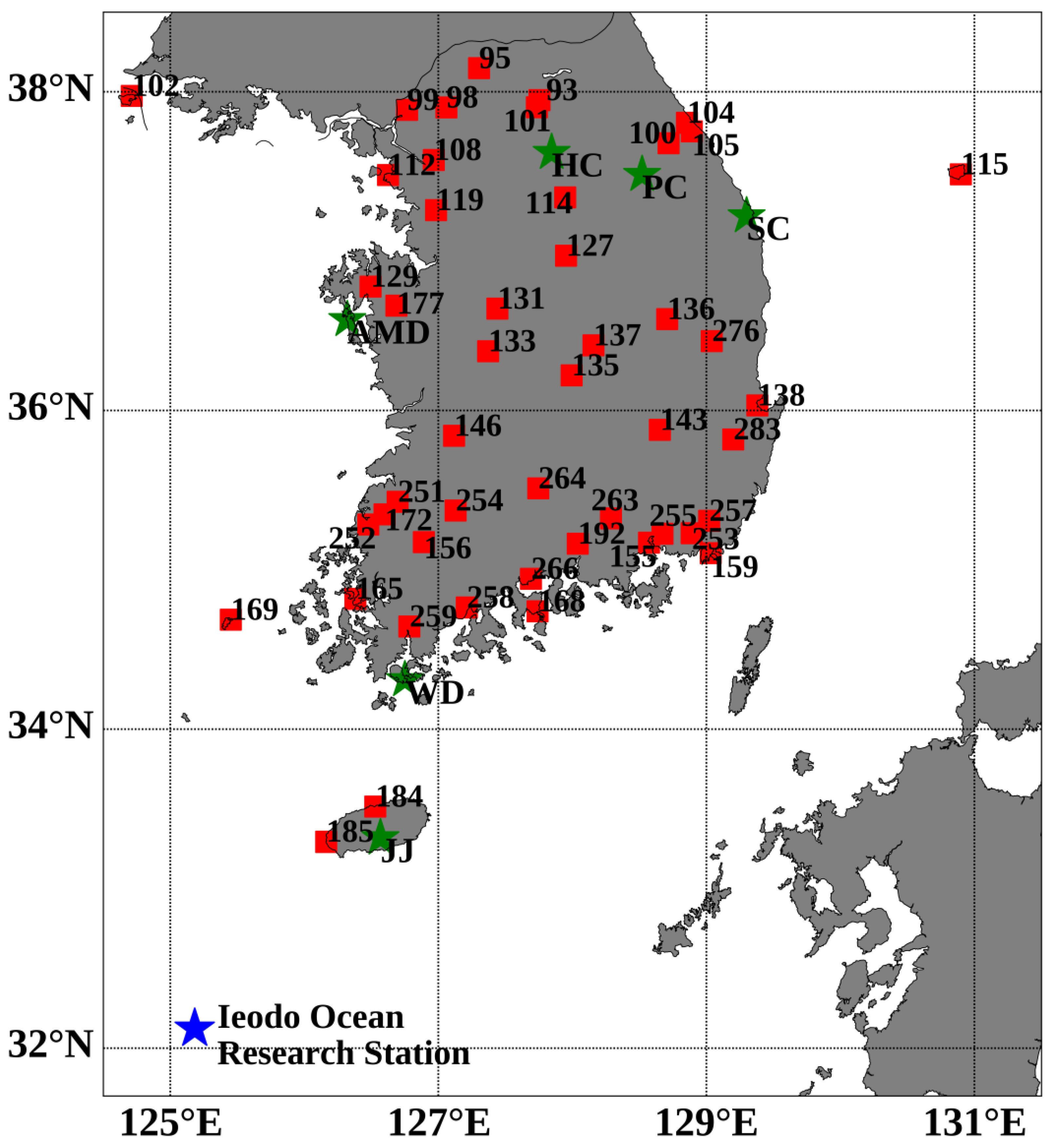
2.2. In Situ Measurements

Solar radiation from space passing through the atmosphere and incident to the land surface can be classified into three categories: direct solar radiation, diffuse solar radiation, and global solar radiation. Direct solar radiation represents the solar radiation that is not scattered and reflected by atmospheric molecules or particulates but is directly incident to the land surface; diffuse solar radiation denotes the solar radiation that arrives at the land surface after scattering or reflection by atmospheric molecules or particulates; global solar radiation is defined as the total solar radiation incident to the land surface as the aggregation of the direct component and the diffuse component. For planning photovoltaic power generation, the global solar radiation must be monitored. Therefore, we calculated the global solar radiation (hereafter referred to as SSI) from the GK2A/AMI using an ML technique.
Because the Korean Peninsula has complicated geographical and meteorological properties, each region has different characteristics affected by SSI. The KMA has established 81 Automated Surface Observing System (ASOS) stations for monitoring meteorological conditions in real time. Among these ASOS stations, only 48 ASOS stations observe SSI in real time using pyranometers every minute (Figure 2). The KMA conducted the quality control of these ASOS pyranometers based on the criteria and guidance provided by the World Meteorological Organization (WMO) to maintain in situ SSI monitoring with high accuracy [26]. Because SSI fluctuates rapidly depending on the weather conditions, quality control is difficult. Thus, the KMA distributes the in situ SSI measurements taken every minute after preprocessing by aggregating the SSI over an hour as the operational data. The hourly SSI ground measurements from ASOS stations were provided as the operational in situ SSI measurements of the KMA and were used to provide reference data for training and validating the ML model (https://data.kma.go.kr/cmmn/main.do, accessed on 17 December 2021).
In order to test the model on other ground-based measurements, we used in situ measurements from the Ieodo Ocean Research Station (IORS) operated by the Korea Hydrographic and Oceanographic Agency (KHOA) and flux towers operated by the National Institute of Forest Science (NIFoS) (Figure 2). IORS was located on 125°10′56” E and 32°07′22” N, 149 km southwest of Jeju Island, in 2003. KHOA operates IORS in real time for monitoring both marine and atmospheric environments every minute (http://www.khoa.go.kr/oceangrid/koofs/kor/oldobservation/obs_past_search.do, accessed on 28 January 2022). NIFoS operates six flux towers over Korea; the flux towers observe the environmental conditions twice every hour (http://know.nifos.go.kr/know/service/flux/fluxIntro.do, accessed on 28 January 2022). The in situ SSI measurements from IORS and the NIFoS flux towers are also quality-controlled according to the criteria of WMO. To use in situ SSI data from IORS and the flux towers for validation, we converted them to hourly SSI by aggregating the SSI over an hour.
The commonly used unit for SSI is W m−2, meaning the radiation energy over unit area and unit time. However, the KMA preprocessed the operational in situ SSI measurements by cumulating them over an hour and converting them to the unit of MJ m−2. The unit of MJ m−2 indicates the radiation energy over the unit area and unit time, similar to W m−2. In this study, the unit of SSI was unified as MJ m−2, which is the standard of the KMA in situ SSI measurements as the reference value of the model. For the in situ SSI data observed from IORS and NIFoS flux towers, after their unit of W m−2 was converted into MJ m−2, the in situ SSI data were used to test the model.

3. Methods

3.1. Data Processing

Figure 3 shows the process to train and test the SSI retrieval model from GK2A/AMI data in this study. We preprocessed the input data and constructed matchups between the satellite data and ground-based in situ SSI. The matchups were classified into training datasets and testing datasets based on the acquisition date. Over approximately a year, from 25 July 2019 to 31 July 2020, the matchups were used as the training dataset for training the ML model. For training the model, we conducted five-fold cross-validation to optimize the ML model; 80% of the training datasets were used for the model training by adjusting parameters in the ML model, and 20% were used to validate the SSI derived from GK2A/AMI based on the ML model for minimizing the loss function and preventing the overfitting of the ML model. For the matchups from 1 August 2020 to 31 January 2022, the testing datasets were used to assess the ML model’s performance. Because the objective of this study was to build an ML model for estimating the operational SSI in real time, the ML model could estimate SSI for a longer period based only on the data for previous training periods. Thus, we did not select the random training and testing dataset for the entire period, but sequentially selected the training and testing dataset.
To estimate SSI from GK2A/AMI data, we used sixteen channels, two background channels, and two static data as input variables. The spectral characteristic of cloud changes depending on the season, surface type, surface temperature, and environmental conditions. By accumulating satellite data for a specific period, it is possible to extract the spectral characteristics of the area under a clear sky. Thus, when using satellite data to detect cloud, it is common to use the background channel that accumulates and produces data for a specific period [25]. Because SSI dramatically depends on the cloud cover, we used two background channels, one visible channel (VIS0.6), and one thermal infrared channel (IR10.5) over 30 days as input variables to improve cloud detection. Furthermore, since SSI varies according to solar radiation, we used extraterrestrial solar radiation (ESR) and SZA as input variables.

3.1.1. Extraterrestrial Solar Radiation (ESR)

Solar radiation carried from space to the top of the atmosphere is called ESR. ESR plays an important role for meteorological parameters and can be estimated using the coordinates of the area, Julian day, and local standard time, as follows [27,28]:
R a = 12 × 60 π G S C d r ( ( ω 2 ω 1 ) sin φ sin δ + cos φ cos δ ( sin ω 2 sin ω 1 ) ) ,
ω 1 = ω π t 1 24 ,
ω 2 = ω + π t 1 24 ,
d r = 1 + 0.033 cos 2 π 365 J ,
δ = 0.409 sin ( 2 π 365 J 1.39 ) ,
ω = π 12 [ ( t + 0.06667 ( L z L m ) + S c ) 12 ] ,
S c = 0.1645 sin 2 b 0.1255 cos b 0.025 sin b ,
b = 2 π ( J 81 ) 364 ,
where Ra and GSC denote ESR (in MJ M−2) and the total solar irradiance, respectively; ω 1 , ω 2 , and ω indicate the solar time angle, an angular measure derived from the Earth’s rotation on the polar axis, at beginning, end, and midpoint of the period (in rad), respectively; d r and J represent the inverse relative Earth–Sun distance and Julian day, respectively; t and t1 refer to the standard time at the midpoint of the period and the length of the period, respectively; φ and δ are latitude and solar declination (in rad), respectively; L z , L m , and S c refer to the longitude of the local time zone, the latitude of the measurement site, and the seasonal correction for solar time, respectively; b indicates the parameter for seasonal variation of solar time. Solar time angle is related to the midpoint of the period corrected by the difference in longitude between the measurement site and local time zone; the longitude of the local time zone indicates the location of the sun at the zenith based on the local standard time. Because ESR indicates the solar radiation incident on the top of the atmosphere, it should be physically greater than or equal to 0. The calculation of and information regarding each parameter are detailed in Allen et al. [27].

3.1.2. Standardization of Input Variables

When input variables are linearly related to each other and the output variable, it is unnecessary to normalize or standardize them for ML model training. Otherwise, when the input variables show a nonlinear relationship with each other and the output variable, the adjusted weights and biases of the model are dramatically affected by the variables at a large magnitude in model training, which degrades the training rate and causes local optimization [29]. Furthermore, utilizing extremely small weights could induce the uncertainties of calculating the floating point with a computer [30]. For resolving these limitations, standardization or normalization is generally used, and there are no fixed methods for standardization and normalization. Using standardized or normalized input variables improves the training rate and reduces the possibility of local optimization. Therefore, we applied standardization to input variables in this study as follows:
V = ( V V m e a n ) V s t d ,
where V denotes the unstandardized input variable; V is defined as the standardized input variable; V m e a n represents the mean value of the input variable; and V s t d refers to the standard deviation of the input variable. When applying the standardization, input variables showed similar ranges and magnitudes.
Because the objective of this study was to build an ML model for the retrieval of SSI in real time, the ML model was trained for the ability to calculate accurate SSI for a longer period based only on the data for previous training periods. Thus, when standardizing the input variables, their mean and standard deviation were calculated based on the training data from 25 July 2019 to 31 July 2020.

3.2. ML Approach

This study aimed to calculate the SSI from GK2A/AMI data using an ML approach. Because in situ SSI measurements consider global solar radiation, it is necessary to characterize not only the direct component but also the diffuse component of solar radiation. Thus, for producing the optimized SSI model, we applied a convolutional neural network (CNN), which could characterize the surrounding environment conditions.
Because the SSI in this study represents global solar radiance, it includes the direct component and diffuse component of solar radiation. For improving the accuracy of SSI measurements from GK2A/AMI, it was useful to account for the nearest cloud and solar conditions and adjacent cloud and solar conditions using the convolution method. CNN trains contextual features of images at different scales. While CNNs were initially developed for image classification, they have recently proven to be effective in various applications related to satellite images, including object detection and super resolution imaging [31,32,33]. A CNN model comprises convolution layers and pooling layers with a number of neurons, and dense layers are often added. We applied a 1d-CNN model, which used a 3-by-3 array of input variables in the input layer and added a flatten layer and dense layer. The 1d-CNN model for extracting the patches in the flattened spectrum vector identifies descriptive local features of adjacent pixels [34]. The 1d-CNN model could be useful for identifying fixed-length signal data such as spectral sequential data and time series data [35].

3.2.1. Hyperparameters

CNNs have a structure wherein layers composed of numerous neurons are interconnected with their weights and biases. Each layer has an activation function that computes output values to neurons in the next layer based on input values from neurons in the previous layer. An optimizer algorithm minimizes the error and maximizes the accuracy of the ML model by adjusting the biases and weights in the network using a feed-forward network and error back-propagation process based on the reference value. In model training, when output values in the neurons of the current layer are calculated based on input values transferred from neurons of the previous layer, the neurons combine the input values via biases and weights, as follows:
o j =   i i w i j b j ,
where o j indicates the net of the weighted input for the jth neuron in the current layer; i i represents the input value transferred from the ith neuron in the previous layer; w i j is the weight connected with the ith neuron in the previous layer and the jth neuron in the current layer; and b j refers to the bias of the jth neuron in the current layer. In order to calculate the final output of the jth neuron in the current layer for transferal to the next layer, o j should be conjugated by an activation function. The activation function could be a discrete or continuous function according to the application field. In this study, the exponential linear unit (ELU) was utilized as an activation function and showed fine performance with good generalization and a high learning rate [36]:
f ( x ) = { x i f   x > 0 α ( exp ( x ) 1 ) i f   x 0 ,  
where x denotes the input value for an activation function and represents o j ; α refers to a hyperparameter of the ELU function that determines the value, where the function converges for negative o j ; and the hyperparameter α of the ELU function is 1.0.
For accelerating the training rate and improving the model performance, the batch normalization layer was applied between each hidden layer [37]. When utilizing the batch normalization layer, the ML model calculates the normalization considering the batch’s dimension; the normalization ensures that the input values of each hidden layer are allocated equally; the accuracy of the model greatly depends on the batch size. As an optimizer algorithm, a method for stochastic optimization (ADAM) was applied, whose hyperparameters had a learning rate of 10−3, a decay of 10−3, an epsilon of 10−7, and a beta1 and beta2 of 0.9 and 0.999, respectively [38]. To train and run the model based on ML approaches, we used TensorFlow back-end in Python.
Even though the atmospheric parameters showed nonlinear relationships with each other, when making the structure of the ML model complex, the ML model could estimate the atmospheric parameters with good performance. To find an optimal CNN model in respect of network structure and parameters, the accuracy of the model with each parameter was analyzed, such as the number of filters, nodes, and layers, and regularization (Table 2). Each parameter was tested by three values with respect to the other parameters, and we employed 16, 32, and 64 filters; 100, 200, and 300 nodes; and 1, 2, and 3 layers. For restraining the overfitting problem of the ML model for the only training dataset, it is common to use regularization, drop-out, and early stopping. L1 regularization and L2 regularization are the most widely used regularization methods [39,40]. The more complex the structure of the ML model, the higher the probability of overfitting problems. The regularization method shrinks the impact of the hidden neurons by reducing the weights during the back-propagation process. Smaller weights reduce the complexity of the model by making some neurons negligible, which generalizes the ML model and avoids overfitting problems. The regularization term of L1 regularization and L2 regularization, called a penalty term, is added to the objective function, reducing the aggregation of the parameters by the absolute value and squares, respectively [41]. When using L1 regularization, the complexity of the model is reduced by causing the important weights in the model to be selected for use, and the other weights are set to zero. In contrast, L2 regularization makes these other weights close to zero but not zero. Due to the characteristics of the regularization methods, in general, L1 regularization is robust in regard to outliers and is commonly used if many features are to be ignored, while L2 regularization is sensitive to outliers and is mainly used in cases where many features are to be considered. When applying a regularization method, the regularization term is adjusted by multiplying the regularization parameter controlling the strength of the penalty [42]. When the regularization parameter is close to 0, the effect of the penalty decreases. In this study, for L1 regularization and L2 regularization, we tested the regularization parameters of 0, 10−5, and 10−3. We analyzed the accuracy of the CNN model depending on the network structure and regularization term, and we selected the optimized CNN model with 64 filters, 300 nodes, 2 layers, and the L1 regularization parameter of 10−5.

3.2.2. Feature Permutation

Although it is difficult to investigate in detail the structure of the ML model in a black-box model such as an artificial neural network, the importance of input variables can be calculated by various methods. In particular, some features (input variables) cannot contribute to improving the accuracy of ML models and only make them more complex. For investigating the trained ML model, a feature permutation test, the most commonly used method, was conducted for each input variable [43]. Feature permutation, initially proposed for Random Forest models, can be widely used for ML models [44]. For conducting the feature permutation test, we randomly permuted the order of one variable and assessed the decrease in the performance of the ML model; we repeatedly conducted this process for all input variables; finally, we calculated the mean decrease in the accuracy for each variable [45]. Because the arrangement of each variable differs from its arrangement when training the model, the performance is generally reduced compared with the accuracy when applying the original order of each variable. A feature with a larger mean decrease in accuracy is a more important feature in the ML model because the data quality of the feature has a greater influence on its performance. If the performance does not decrease significantly when a specific feature is permutated, it can be assumed that the feature is unimportant to the ML model or that the information in the feature is included in the other features [46]. In this study, when each variable was randomly permutated and applied to the model, the increase in the root mean square error (RMSE) was calculated as the decrease in its accuracy. We repeated the permutation test 10 times to calculate the mean decrease in accuracy with each input variable and ranked the input variables with respect to their mean decrease in accuracy.

3.3. Statistical Analysis

Hourly SSI estimated using ML approaches was compared with in situ hourly SSI. For quantitative evaluation of the hourly SSI derived from GK2A/AMI, we used the bias, RMSE, mean absolute error (MAE), normalized RMSE (nRMSE), and Pearson’s correlation coefficient (R), as follows:
Bias = 1 N i = 1 N ( E s t i O b s i ) ,
RMSE = i = 1 N ( E s t i O b s i ) 2 N ,
MAE = 1 N i = 1 N | E s t i O b s i | ,
nRMSE = i = 1 N ( E s t i O b s i ) 2 N i = 1 N O b s i N ,
R = i = 1 N ( E s t i E s t ¯ ) ( O b s i O b s ¯ ) i = 1 N ( E s t i E s t ¯ ) 2 i = 1 N ( O b s i O b s ¯ ) 2 ,
where and O b s i represent the estimated SSI from satellite data and observed SSI from the ground station, respectively; N is the number of data points; the subscript i denotes the i th data point; and E s t ¯ and O b s ¯ represent the mean of the estimated SSI from satellite data and observed SSI from the ground station, respectively.

4. Results

4.1. Input Data Correlations

Figure 4 shows the correlation coefficients of the input variables used for estimating the hourly SSI and the ground-based SSI measurements from the KMA ASOS stations in different datasets. Except for the SZA, all input variables (19 input variables) showed a positive correlation coefficient with hourly SSI from the KMA ASOS stations. For intense cloud conditions, even if the ESR was high, the SSI was observed to be low; however, for clear sky conditions, the SSI increased as the ESR increased. Furthermore, the SSI was consistently observed to be 0 at nighttime, with an ESR of 0. The ESR changes depending on environmental conditions such as the Earth–Sun distance, the solar elevation, and the solar activity. The higher the solar activity, the closer the Earth–Sun distance, and the higher the solar elevation, the higher the ESR value. Hence, the ESR showed the highest correlation coefficient (0.74). Because the 3.8 μm channel is a useful channel for detecting low clouds and fog, a high brightness temperature indicates no fog and low clouds, and a high SSI is measured under clear sky conditions. Hence, among the input variables related to the channel, IR3.8 showed the highest correlation coefficient (0.61). Conversely, only the SZA showed a negative correlation coefficient (−0.74), because the SZA was highly inversely correlated with an ESR of −0.98. As the SZA decreased, the solar altitude increased; hence, the ESR increased, which increased the SSI. In addition, with an SZA above 90 degrees at nighttime, the SSI was consistently observed to be 0. The 1.6 μm channel and 1.3 μm channel are solar channels that show only at daytime and show a high reflectance for cloud area at daytime, like the visible channels. Furthermore, because the 1.6 μm channel had an ability to distinguish water-based clouds from a snow-covered surface and depict the land surface, it showed a higher correlation coefficient (0.57) than the visible channels. However, although the 1.3 μm channel had the ability to detect cirrus clouds, it could not depict the land surface, so it showed the correlation coefficient closest to 0, with a value of 0.06, compared with the other input variables.

4.2. Training History

Figure 5 presents the training history of the CNN model with respect to epochs, indicating the number of cycles that the model was trained for all training datasets. An epoch represents that the weights of the model are updated by the entire training dataset at one time. In order to optimize the biases and weights of the neurons in each layer of the ML model, it was trained for minimizing the loss function. The CNN model showed that the RMSE and MAE rapidly decreased. Up to the epochs of 60, the RMSE and MAE of the CNN model rapidly decreased in both the training datasets and validation datasets as the epochs increased. Above the training epochs of 60, the RMSE and MAE of the CNN model were slightly improved, and when the training epochs reached 100, the changes in the RMSE and MAE were almost negligible for both the training and validation data sets.

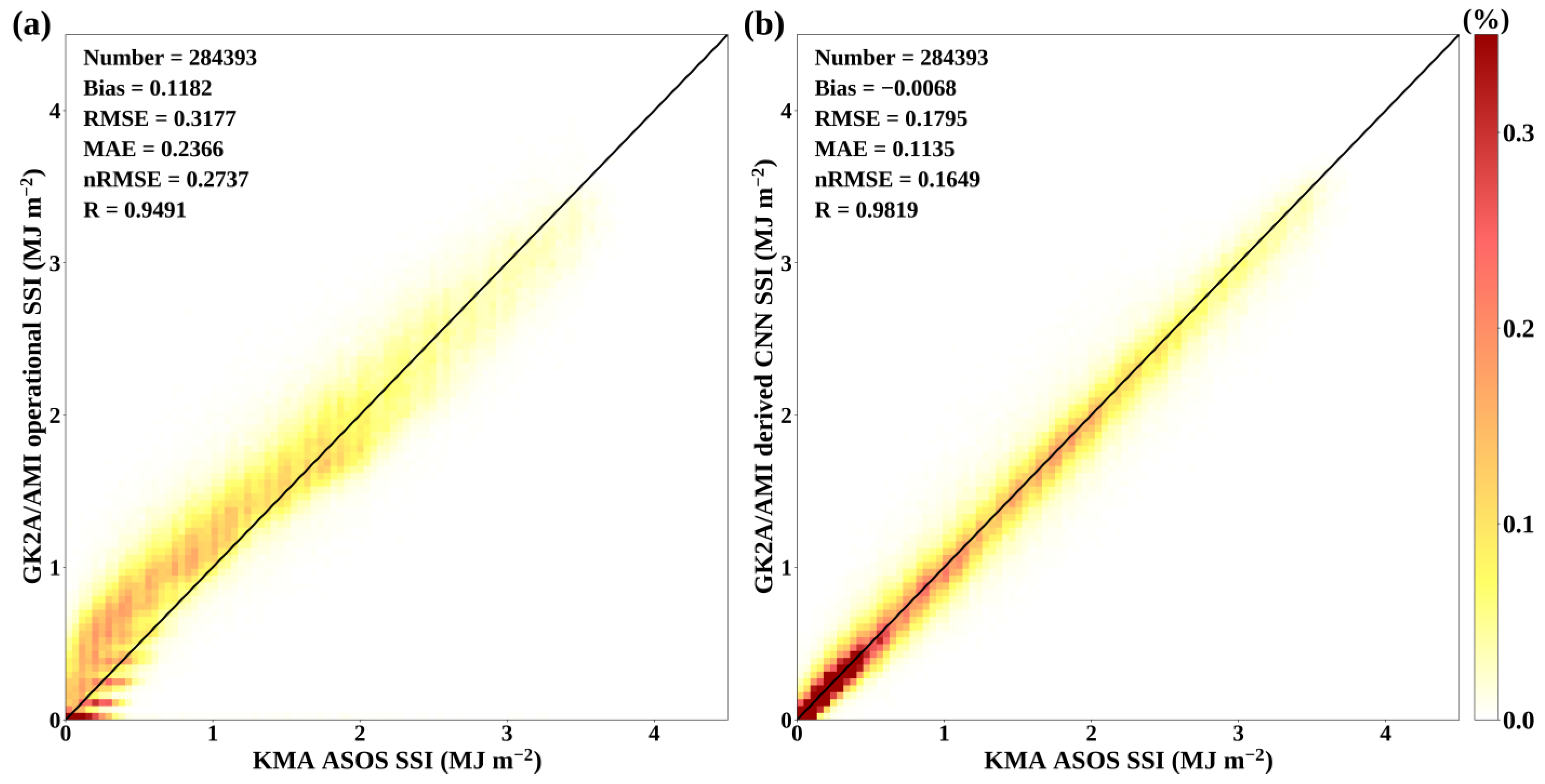
4.3. Evaluation against KMA ASOS Stations

Based on the theoretical principle and lookup table, the SSI had been derived from the GK2A/AMI as an operational product in real time. Therefore, to evaluate the accuracy of the CNN model for estimating the SSI around Korea in this study, the accuracy of the GK2A/AMI operational SSI was simultaneously verified. For quantitative validation, we compared the hourly GK2A/AMI-derived SSI based on the CNN and the operational GK2A/AMI-derived SSI around Korea with the in situ SSI measured by the KMA ASOS stations from 1 August 2020 to 31 January 2022 (Figure 6). The total number of data matchups was 284,393. The accuracy of the hourly SSI derived from the GK2A/AMI operational algorithm showed an RMSE of 0.318 MJ m−2 and a Pearson’s R of 0.949; however, the accuracy of the hourly SSI derived from the CNN model showed an RMSE of 0.180 MJ m−2 and a Pearson’s R of 0.982, which indicated that the ML approach showed higher accuracies compared to the GK2A/AMI operational algorithm. Regarding bias, the GK2A/AMI operational algorithm tended to overestimate the SSI as compared to the in situ measurements, with a bias of 0.118 MJ m−2. Otherwise, the CNN model tended to underestimate the SSI, showing biases of −0.007 MJ m−2. Regardless of positive and negative bias, the magnitude of the bias errors was larger in the GK2A/AMI operational algorithm, which indicated that the CNN model showed better performance considering bias errors.
For the period from 1 August 2020 to 31 January 2022, we verified the accuracy of the GK2A/AMI hourly SSI, as derived from the operational algorithm and the CNN model, by comparing them with in situ SSI measurements from each KMA ASOS station (Figure 7). For the operational algorithm, the RMSE values ranged from 0.210 MJ m−2 (at station 99) to 0.420 MJ m−2 (at station 185); the bias ranged from 0.008 MJ m−2 (at station 165) to 0.323 MJ m−2 (at station 185); and the Pearson’s R ranged from 0.924 (at station 115) to 0.967 (at station 185). Conversely, for the CNN model, the RMSE values ranged from 0.091 MJ m−2 (at station 137) to 0.314 MJ m−2 (at station 169); the bias ranged from −0.082 MJ m−2 (at station 102) to 0.051 MJ m−2 (at station 146); and the Pearson’s R ranged from 0.946 (at station 169) to 0.991 (at station 137). Overall, the CNN model showed lower RMSEs and higher R values than the operational algorithm at all KMA ASOS stations, which indicates that the CNN model estimated the SSI more accurately. In particular, at stations 115, 169, and 172 (hereafter referred to as group 1), regardless of the model, high RMSEs and low values of Pearson’s R were observed compared to other stations. In contrast, at stations 112, 168, 184, and 185 (hereafter referred to as group 2), the CNN showed a low RMSE, and the operational algorithm showed a high RMSE, which could have been caused by a high positive bias.
Station 172 was located over land between station 251 and station 252. Although the stations among group 1 and 2, excluding station 172, were located over coastal regions or islands, they showed good performance. Therefore, the low performance for group 1 and 2 was not due to the impact from nearby water. The operational product of GK2A/AMI estimated the SSI not by considering neighboring pixels but based only on the pixel equivalent to the area. However, the CNN model characterized the surrounding environment based on neighboring pixels. Group 2 showed high and low accuracy for the CNN model and operational algorithm, respectively, which was believed to be caused by the surrounding environment, due to the regional characteristics that greatly affected the stations. However, group 1 showed low accuracy regardless of the model; the in situ SSI measurements from these stations showed low quality over the testing period from 1 August 2021 to 31 January 2022.

4.4. Evaluation against KHOA IORS and NIFoS Flux Towers

As the GK2A/AMI hourly SSI model using the CNN method was trained using only the ground-based SSI measurements from the KMA ASOS stations, it was necessary to inspect the applicability of the estimated hourly CNN SSI from GK2A/AMI by comparing it with ground-based SSI measurements from the KHOA IORS and NIFoS flux towers for the period from 1 August 2020 to 31 January 2022 (Figure 8). The KHOA IORS and NIFoS flux towers measured the SSI every minute and every 30 min, respectively, and we derived hourly SSI using only those in situ SSI data for which there were no missing data over an hour. In situ hourly SSI from the KHOA IORS and NIFoS flux towers ranged from 0.001 MJ m−2 to 4.017 MJ m−2, and GK2A/AMI-derived CNN hourly SSI ranged from 0.0 MJ m−2 to 3.638 MJ m−2. Compared with the in situ hourly SSI, the total number of data matchups was 36,246, and the GK2A/AMI-derived CNN hourly SSI showed accuracies of 0.328 MJ m−2 (RMSE), 0.252 MJ m−2 (MAE), 0.326 MJ m−2 (STD), and −0.038 MJ m−2 (bias), with an nRMSE of 0.269, indicating that the CNN-based hourly SSI retrieval model had a tendency to underestimate the SSI relative to the ground-based SSI measurements from the KHOA IORS and NIFoS flux towers overall. In particular, for an SSI of less than 2.0 MJ m−2, the GK2A/AMI-derived CNN hourly SSI showed accuracies of 0.321 MJ m−2 (RMSE) and 0.011 MJ m−2 (bias), indicating that its tendency to underestimate SSI weakened under low-SSI conditions. However, for an SSI greater than 2.0 MJ m−2, the RMSE and bias were 0.350 MJ m−2 and −0.195 MJ m−2, respectively, implying that the tendency to underestimate SSI intensified under high-SSI conditions. The characteristic that the tendency of the CNN model to underestimate became stronger as the SSI increased was also found through the regression line, whose slope was 0.8785 (less than 1) and bias 0.1105 (greater than 0). Because the CNN model was trained based only on the KMA ASOS stations, the estimated SSI from the CNN model could be optimized for the Korean Peninsula. Furthermore, the CNN model showed a different tendency depending on the magnitude of SSI. Therefore, when applying the CNN model for other regions, it is necessary to consider its tendencies. For low-latitude regions, where a high SSI is more frequent, the underestimation by the model would be more apparent; for high-latitude regions, where a low SSI is more frequent, the underestimation by the model would weaken. Although the CNN-based SSI model showed an underestimation of SSI compared to the in situ SSI values from the KHOA IORS, the Pearson’s R was 0.939 for the overall SSI, indicating that the CNN-based hourly SSI retrieval model accurately estimated the in situ SSI from the KHOA IORS, overall.

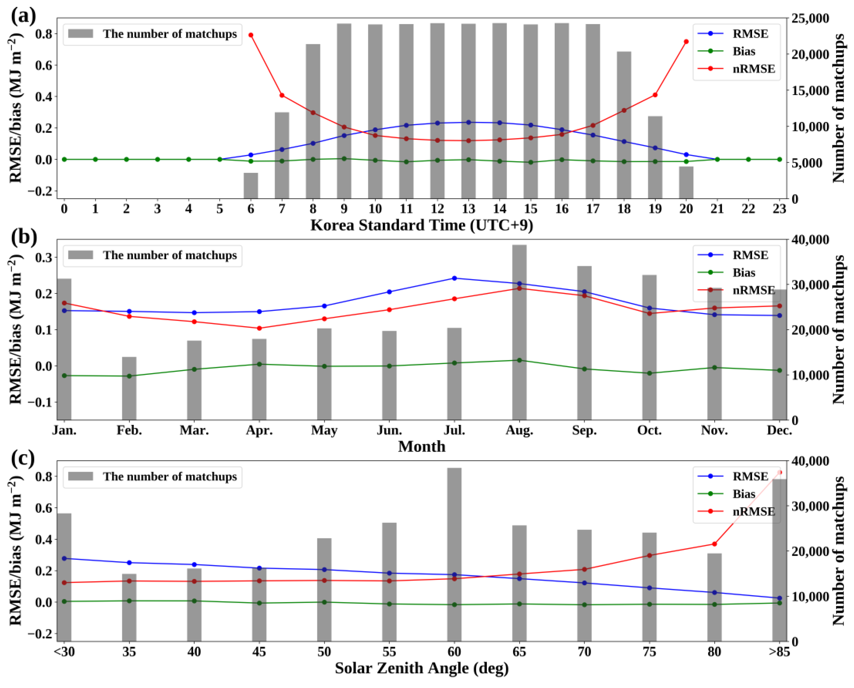
4.5. Error Characteristics

To investigate the effect of observation time on the GK2A/AMI-derived CNN SSI error, we examined the error with respect to Korean Standard Time (KST, UTC+9), month, and SZA (Figure 9). The local time showed an RMSE of 0.24 MJ m−2 or less, and the opposite changes between RMSE and nRMSE overall (Figure 9a). Korea’s solar solstice occurs at approximately 12:30 KST, and the sun rises before and sets after this time. Thus, as the solar altitude increases up until 12:30 KST, the amount of ESR also increases; hence, the amplitude of SSI error increases. In contrast, as the solar altitude decreases after 12:30 KST, the amount of ESR also decreases, so the amplitude of the SSI error decreases. As a result, the RMSE increased up until 12:00 KST, and the RMSE decreased after 13:00 KST. Conversely, as the relative accuracy parameter, the nRMSE indicated the lowest value (0.12) at 13:00 KST and high values at the time before sunrise and sunset (Figure 9a). As shown in Figure 9b, it showed an RMSE of 0.25 MJ m−2 or less and similar changes between RMSE and nRMSE overall. In warm seasons (August to September), a high RMSE (0.205 MJ m−2) and a nRMSE higher than and 0.194 were shown, but in April, a low RMSE and nRMSE of 0.150 MJ m−2 and 0.104, were observed, respectively. Considering that RMSE and nRMSE showed similar trends, this was not due to the amount of ESR. Due to the Korean Peninsula’s monsoon, broad and thick clouds are frequent in summer, and clear skies are common in spring [47]. As a result, the SSI is contaminated by intense clouds in the summer, and in spring, its accuracy is improved by frequent clear skies. As the SZA increased, it was found that the RMSE decreased and the nRMSE increased (Figure 9c). As the SZA decreased, the amplitude of the ESR and SSI increased, so its RMSE increased. In addition, because it was close to noon, the variation of the SSI according to the change in SZA was low, so the SSI showed high accuracy, with a low nRMSE of 0.124 at an SZA of less than 30 degrees. In contrast, as the SZA increased and the observation time approached sunset and sun rise, the variation in SSI according to the change in SZA was high, so the SSI showed low accuracy, with a high nRMSE of 0.825 at an SZA of more than 85 degrees. Since the ESR was absolutely affected by the SZA, the error characteristic was evident in the SZA. Conversely, because the time of the sunrise and sunset and the SZA according to the local time varies with season, the ESR and SZA would seasonally change even at the same local time. Therefore, the error characteristic shown in Figure 9a differs from the error characteristic shown in Figure 9c.
Furthermore, to examine the effect of the observation environment on the GK2A/AMI-derived CNN SSI error, we examined the error with respect to in situ SSI, visibility, daylight, and cloud amount (Figure 10). In terms of in situ SSI, it was found that the bias and nRMSE decreased and the RMSE approximately increased as the in situ SSI increased (Figure 10a). As the in situ SSI increased, the amplitude of the SSI increased, so the RMSE increased and the nRMSE decreased. As a result, the RMSE and nRMSE were 0.094 MJ m−2 and 0.689 at an in situ SSI of less than 0.2 MJ m−2, respectively, and the RMSE and nRMSE were 0.250 MJ m−2 and 0.074 at an in situ SSI of more than 3.4 MJ m−2, respectively. A negative bias was shown at an in situ SSI of higher than 2.0 MJ m−2, which indicates that the CNN-based SSI model from the GK2A/AMI underestimated under high-SSI conditions. The tendency of the CNN model to underestimate became stronger as the SSI increased, and an SSI of higher than 3.4 MJ m−2 showed a clear negative bias of −0.137 MJ m−2. As shown in Figure 10b, as the visibility increased, the nRMSE decreased. In particular, the tendency of the CNN model to overestimate was more pronounced as the visibility decreased, and a visibility of lower than 2 km showed a positive bias of 0.037 MJ m−2 and a high nRMSE of 0.404. As the visibility increased, the RMSE increased, and at a visibility of more than 20 km, the RMSE and nRMSE were 0.198 MJ m−2 and 0.158, respectively. In situ daylight refers to the amount of time during which direct solar radiation arrives at the station over the course of an hour; a daylight of 0.5 means that there is direct solar radiation incident to the station for 30 min or 0.5 h. In the terms of in situ daylight, as the daylight increased, the bias and nRMSE decreased (Figure 10c). In high-daylight conditions of more than 0.8 h, the model tended to underestimate, and its bias was less than −0.02 MJ m−2. The nRMSE was 0.437 at a low daylight of 0 h and 0.092 at a high daylight of 1 h. The in situ cloud amount (unitless variable) indicates the fraction of the sky covered by clouds over the regions around the station; a cloud amount of 5 specifies that half of the sky is covered by clouds. As the cloud amount increased, the RMSE increased, although for specific cloud amounts of more than 9 the nRMSE clearly increased (Figure 10d). As the cloud amount increases, the proportion of direct SSI and scattered SSI in the global SSI generally decreases and increases, respectively, depending on cloud distribution. Conversely, satellites estimate the SSI by calculating the degree of attenuation of the ESR by atmospheric elements, including clouds and aerosols, in the corresponding pixel. Thus, the accuracy of the GK2A/AMI-derived SSI decreases when the proportion of scattered radiation increases due to high-cloud-amount conditions [48,49]. In high-cloud-amount conditions of more than 9, however, the RMSE and nRMSE decreased and increased, respectively. This was not because the accuracy of the CNN model increased, but because the amount of SSI decreased. The accuracy had an RMSE of 0.141 MJ m−2 and an nRMSE of 0.335 at a high cloud amount of 10.

5. Discussions

5.1. Feature Permutation

We conducted a feature permutation test for the CNN model to understand the extent to which each input variable influenced the performance of the model when estimating SSI from GK2A/AMI data (Figure 11). The ESR, with the highest mean decrease in accuracy, was ranked as the most important feature. When the ESR was randomly permutated, the RMSE of the CNN model increased to 1.219 MJ m−2. If a clear sky occurs, because there is no sky covered by clouds, when the ESR is incident on the Earth’s surface, it is not affected by clouds. Thus, in clear-sky conditions, the SSI increases as the ESR increased. Furthermore, unless the sky is obscured by thick clouds, a higher ESR generally increases the SSI, even if scattered SSI is considered, and direct SSI cannot theoretically exceed the ESR. Hence, because ESR absolutely affects SSI, it was demonstrated to be the most important feature in the CNN model. The CNN model had the second and third highest feature permutations of 0.959 MJ m−2 (IR12.3) and 0.926 MJ m−2 (IR13.3), respectively, and their difference from the ESR was small compared with the other feature permutations. This implied that the structure of the CNN model was closely related to the ESR and the other input variables, such as IR12.3 and IR13.3, which implies that the structure of the model was complex. Among the top three most important features, including the ESR, the CNN model included infrared channels. Because the SSI is a parameter affected by clouds and atmospheric factors including aerosols, the model should reflect cloud attenuation and atmospheric factors. To reflect atmospheric attenuation, the CNN model was trained with an increased focus on infrared channels.

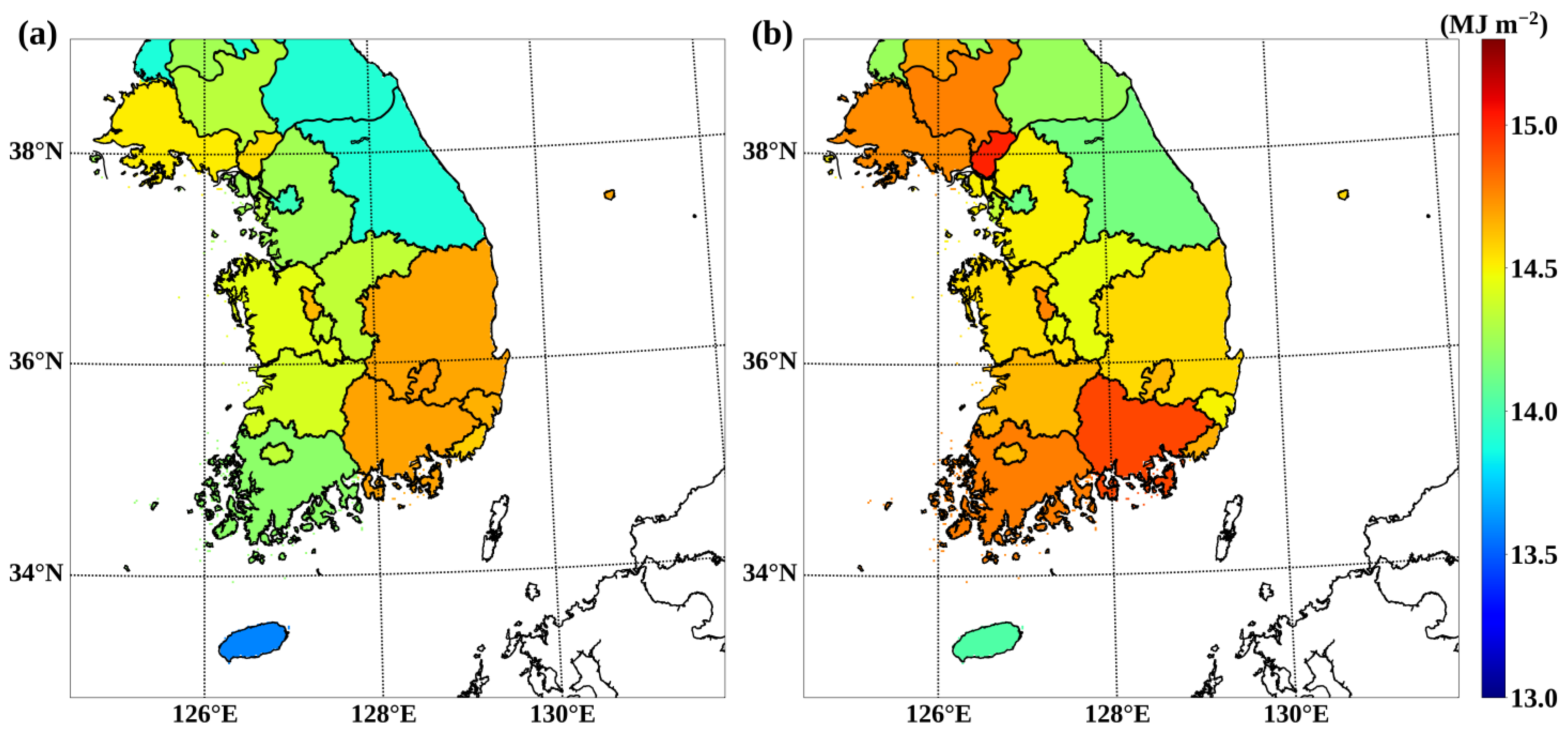
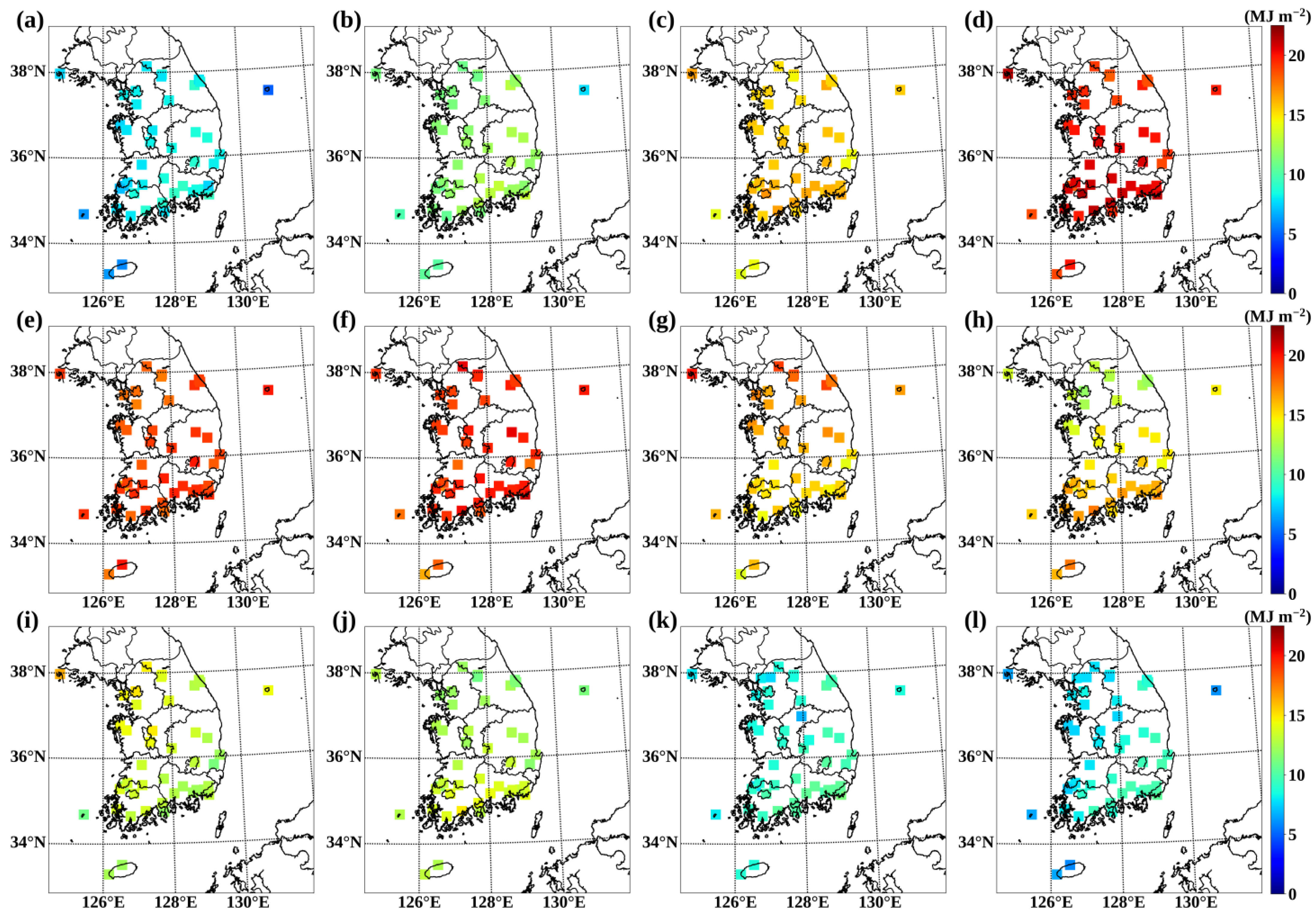
5.2. Spatial Distribution of SSI around Korea
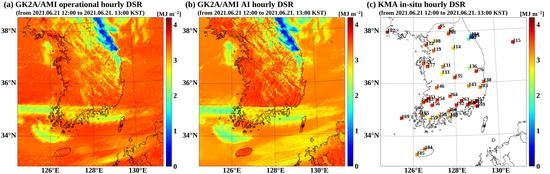
5.2.1. GK2A/AMI SSI

SSI is a key factor in climatological, agricultural, and renewable energy applications. To apply SSI data in these studies and fields, it is essential to understand the spatial and temporal distribution of SSI. Thus, we produced GK2A/AMI-derived CNN-based daily SSI measurements by accumulating hourly SSI for an SZA of less than 80 degrees from 1 January 2020 to 31 December 2021. Based on the daily SSI, the monthly mean daily SSI was calculated for each administrative district over Korea (Figure 12). Among the monthly mean daily SSI values over Korea, the largest value (20.451 MJ m−2) and the smallest value (8.400 MJ m−2) were observed in April and January, respectively (Table 3). The period of April to June showed higher mean daily SSI values compared with other periods. Under a clear sky, the SSI generally increased as the amount of ESR increased, and the ESR increased and decreased in summer and winter, respectively. However, because the Korean Peninsula has a monsoon climate, the coverage and intensity of clouds increases as summer approaches, and the incident solar radiation is reduced by clouds [50,51,52]. In contrast, from late spring to early summer, before the summer monsoon starts, a high SZA and clear skies are usually observed. Hence, around Korea, from July to September, the SSI was affected by intense clouds, and a low mean daily SSI was observed compared with the period of April to June.
The north–south gradient of SSI over Korea reversed in July and August. The GK2A/AMI-derived SSI was higher in the northern region on July; however, the SSI was higher in the southern region in August. In summer, the monsoon front around Korea is affected by air masses such as the North Pacific High over a low latitude and the Okhotsk High over a high latitude. In early summer, i.e., late June and early July, the Okhotsk High is generally stronger than the North Pacific High; thus, the monsoon front is located over the southern region of Korea [53]. However, in late summer, i.e., late July and early August, when the North Pacific High is strong, the monsoon front moves northward and is located over the northern region of Korea [54]. Therefore, in July, the southern regions are generally affected by clouds derived from the monsoon front and show lower SSI than the northern regions; in August, the northern regions are generally affected by clouds derived from the monsoon front and show lower SSI than the southern regions.
The annual mean daily SSI for 2020 and 2021 was calculated at SZA values of less than 80 degrees (Figure 13). The annual mean daily SSI over Korea in 2020 and 2021 was 14.351 MJ m−2 and 14.536 MJ m−2, respectively. Except for some provinces, most administrative districts showed a higher SSI in 2021 than in 2020. Because the Korean Peninsula has a monsoon climate, the Korean summer rainfall system known as Changma occurs and is accompanied by intense clouds and consecutive days of heavy precipitation from mid-June to early September [55]. More specifically, Korea was affected by 15 consecutive heavy rainfall events for the period from mid-June to early September in 2020, and record-breaking rainfall events were reported by KMA [56]. The heavy rainfall events over Korea during Changma are common due to the monsoon climate; however, the intensities and durations of the rainfall in 2020 were higher than normal. This extreme summer rainfall was accompanied by intense cloud coverage and caused a sharp decrease in the mean daily SSI values. Conversely, there were fewer heavy rainfall events in 2021 than in 2020, which caused the mean daily SSI to be higher in 2021 than in 2020.

5.2.2. KMA ASOS SSI

In order to investigate the difference between in situ SSI and satellite-derived SSI according to spatial and temporal distribution, we derived the KMA ASOS-observed daily SSI by accumulating the hourly SSI for an SZA of less than 80 degrees from 1 January 2020 to 31 December 2021 (Figure 14). The maximum and minimum values of the monthly mean daily KMA ASOS in situ SSI are shown in Table 4. In the case of the minimum value of the monthly daily in situ SSI, like the results of the GK2A/AMI-derived CNN-based SSI, the period from April to June showed higher mean daily SSI values compared with other periods, especially July. In terms of spatial and temporal distribution, like the results of the GK2A/AMI-derived CNN-based SSI, from July to September, the mean daily in situ SSI was lower compared with the period from April to June; it was found that the north–south gradient of the SSI over Korea was reversed in July and August.
Despite these similar result with the GK2A/AMI-derived SSI, some characteristics were different. Some stations showed different values from neighboring stations. Although stations 131 and 133 are located near to each other, their mean daily SSI measurements were different for specific months, including July, August, and September. This characteristic was also shown in stations 100, 104, 105, 138, and 283. Furthermore, in terms of the maximum value of the mean daily in situ SSI, unlike the results of the GK2A/AMI-derived CNN-based SSI, the period of April to June showed monthly daily SSI values similar to those of July. These differences between the in situ SSI and the GK2A/AMI-derived SSI could be caused by the observation method. When a satellite observes the Earth, the pixel is interpreted as having homogeneous conditions; the GK2A/AMI collects the environmental conditions of the pixels with a spatial resolution of 2 km, assuming homogeneous conditions. However, the actual cloud conditions, which directly affect SSI, are often heterogeneous. Furthermore, although the satellite measures the SSI based on two-dimensional observations, the in situ SSI observed from ground-based pyranometers is affected by three-dimensional radiative effects and small-scale cloud conditions [57]. These different observations would be slightly alleviated by using hourly SSI; however, for estimating SSI from satellite data, it is impossible to completely exclude the different methods.

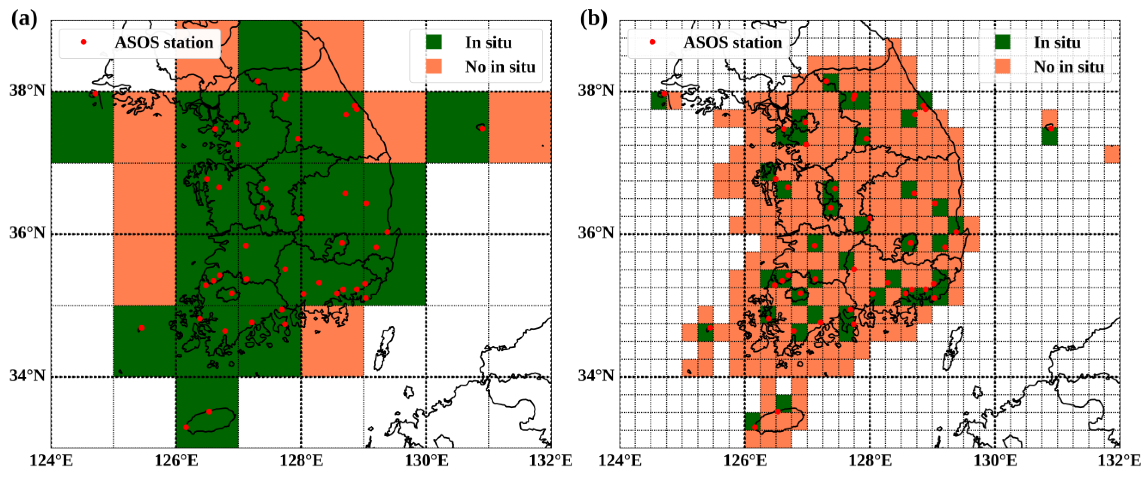
5.3. Gap in the In Situ SSI

To apply SSI data for climatological monitoring, the WMO recommends an ideal spatial resolution of 25 km and a minimum spatial resolution of 100 km [58]. Korea has an area of approximately 120,000 km2, and its coverage, including islands and land areas, can be divided into 258 grid points with 25 km resolution and 26 grid points with 100 km resolution (Figure 15). When monitoring Korea for climatological application using only in situ measurements, at a minimum resolution of 100 km, data are obtained for 18 grid points (approximately 69.2%); at an ideal resolution of 25 km, data are obtained for 41 grid points (approximately 15.9%). If climatological monitoring over Korea is required at the minimum resolution, most areas, except for some regions near shorelines, borders, and islands, are covered by in situ observations (Figure 15a). In contrast, when we aim to meet climatological monitoring requirements at the ideal resolution, most areas over Korea would be missed by in situ observations (Figure 15b). For accurately investigating the climatology of Korea, installing more in situ measurement stations is necessary; however, this is limited by the available human and physical resources. The GK2A/AMI-derived SSI data showed good performance in terms of temporal and spatial stability, and there were no limitations to data acquisition and spatial coverage at a high temporal resolution. Compared with the numerical model data, the satellite-derived SSI exhibited a higher agreement with the in situ SSI; this was because spatially and temporally continuous remote-sensed observations were available [59,60]. Therefore, satellite-derived SSI data can be used as an alternative to in situ SSI measurements for diverse applications, including climatology, renewable energy, and agriculture.

6. Conclusions

For producing an SSI distribution with high accuracy, we developed a model estimating SSI from the GK2A/AMI. We used sixteen channel data and two background-channel data for 30 days from the GK2A/AMI, SZA, and ESR as input data for the ML model. The in situ SSI measurements from 44 ASOS stations operated by KMA were used as reference data. Because the SSI indicates the global solar radiance, including the direct component and the diffuse component of solar radiance, in order to obtain the optimal model from the GK2A/AMI over Korea, we used the CNN model characterizing the surrounding environmental conditions based on neighboring pixels. We trained the model based on the data for the period from 25 July 2019 to 31 July 2020 and assessed the model based on the data after 1 August 2020. As a result of the statistical verification, the CNN model was the model that most accurately estimated the SSI, and the accuracy had an RMSE of 0.202 MJ m−2, a bias of 0.002 MJ m−2, and a Pearson’s R of 0.979. To investigate the efficiency of the estimated CNN SSI from the GK2A/AMI, it was compared with the ground-based SSI from the KHOA IORS and NIFoS flux towers and indicated a good agreement with the in situ SSI.
The CNN SSI showed an evident tendency to underestimate under an in situ SSI of more than 2.0 MJ m−2. As the SZA increased, it was found that the RMSE decreased and the nRMSE increased, and underestimation under an SZA of more than 60 degrees was observed. As the visibility increased, the bias and nRMSE decreased. In particular, the tendency to overestimate was more pronounced as the visibility decreased, and a visibility of lower than 2 km showed a clear positive bias of 0.07 MJ m−2 and a high nRMSE of 0.74. Furthermore, as the cloud amount increased, the nRMSE increased, and the nRMSE was 0.37 at a cloud amount of 10.
The ESR was the most important feature for training the model. The CNN model was trained by focusing on infrared channels and those closely related to ESR and other features. Considering the local characteristics, a high monthly mean daily SSI was observed from April to June due to the Korean Peninsula’s monsoon climate. Furthermore, because the Korean summer rainfall system, Changma, lasted for a longer period in 2020 than in 2021, the annual mean daily SSI was higher in 2021 than in 2020 due to the fluctuation of the SSI depending on the cloud conditions.
The Korean Peninsula has a complex topography and land type, which causes difficulty in providing spatial information for SSI using only in situ measurements. Conversely, because the GK2A/AMI can monitor the environment with a high spatiotemporal resolution, the GK2A/AMI is a suitable tool for monitoring SSI in real time and complementing the gap in in situ measurements. It is thought that two-dimensional SSI information derived from the GK2A/AMI is a useful parameter for climatological and agricultural applications and also for designing solar power systems and smart cities. Future studies will attempt to examine the climatological SSI with other satellite-derived SSI measurements and estimate solar power production using GK2A/AMI-derived SSI. In addition, if it could reflect the seasonal effect by standardizing each spectral channel using ESR, it is possible to simplify the model and accelerate the testing and running of the model. Further studies to simplify the model are necessary, such as by reducing the complexity of the model and the number of input variables. We expect that this study will contribute to renewable energy applications based on satellite data, developing ML approaches using ground-based data and satellite data, and understanding air–land interactions.

Author Contributions

Conceptualization, methodology, validation, and writing (original draft preparation)—J.-C.J.; writing (review and editing)—J.-C.J., E.-H.S. and K.-H.P. All authors have read and agreed to the published version of the manuscript.

Funding

This work was funded by the Korea Meteorological Administration’s Research and Development Program, “Technical Development on Weather Forecast Support and Convergence Service using Meteorological Satellites”, under grant KMA2020-00120.

Institutional Review Board Statement

Not applicable.

Informed Consent Statement

Not applicable.

Data Availability Statement

GK-2A/AMI data used in this study are available on http://datasvc.nmsc.kma.go.kr/datasvc/html/main/main.do?lang=en (accessed on 17 December 2021). In situ SSI measurements from KMA ASOS stations used in this study are available on https://data.kma.go.kr/cmmn/main.do (accessed on 17 December 2021). In situ SSI measurements from KHOA IORS and NIFoS flux towers used in this study are available on http://www.khoa.go.kr/oceangrid/koofs/kor/oldobservation/obs_past_search.do and http://know.nifos.go.kr/know/service/flux/fluxIntro.do, respectively (accessed on 28 January 2022).

Conflicts of Interest

The authors declare no conflict of interest.

References

  1. Chen, L.; Yan, G.; Wang, T.; Ren, H.; Calbó, J.; Zhao, J.; McKenzie, R. Estimation of surface shortwave radiation components under all sky conditions: Modeling and sensitivity analysis. Remote Sens. Environ. 2012, 123, 457–469. [Google Scholar] [CrossRef]
  2. Kalnay, E.; Kanamitsu, M.; Kistler, R.; Collins, W.; Deaven, D.; Gandin, L.; Iredell, M.; Saha, S.; White, G.; Woollen, J.; et al. The NCEP/NCAR 40-year reanalysis project. Bull. Am. Meteorol. Soc. 1996, 77, 437–471. [Google Scholar] [CrossRef] [Green Version]
  3. Trenberth, K.E.; Fasullo, J.T.; Kiehl, J. Earth’s global energy budget. Bull. Am. Meteorol. Soc. 2009, 90, 311–323. [Google Scholar] [CrossRef]
  4. Wang, H.; Pinker, R.T. Shortwave radiative fluxes from MODIS: Model development and implementation. J. Geophys. Res. Atmos. 2009, 114, D20201. [Google Scholar] [CrossRef]
  5. Mueller, R.W.; Matsoukas, C.; Gratzki, A.; Behr, H.D.; Hollmann, R. The CM-SAF operational scheme for the satellite based retrieval of solar surface irradiance—A LUT based eigenvector hybrid approach. Remote Sens. Environ. 2009, 113, 1012–1024. [Google Scholar] [CrossRef]
  6. Liang, S.; Zhao, X.; Liu, S.; Yuan, W.; Cheng, X.; Xiao, Z.; Zhang, X.; Liu, Q.; Cheng, J.; Tang, H.; et al. A long-term Global Land Surface Satellite (GLASS) data-set for environmental studies. Int. J. Digit. Earth 2013, 6, 5–33. [Google Scholar] [CrossRef]
  7. Wang, Y.; Buermann, W.; Stenberg, P.; Smolander, H.; Häme, T.; Tian, Y.; Hu, J.; Knyazikhin, Y.; Myneni, R.B. A new parameterization of canopy spectral response to incident solar radiation: Case study with hyperspectral data from pine dominant forest. Remote Sens. Environ. 2003, 85, 304–315. [Google Scholar] [CrossRef]
  8. Ye, Z.X.; Cheng, W.M.; Zhao, Z.Q.; Guo, J.Y.; Ding, H.; Wang, N. Interannual and seasonal vegetation changes and influencing factors in the extra-high mountainous areas of Southern Tibet. Remote Sens. 2019, 11, 1392. [Google Scholar] [CrossRef] [Green Version]
  9. Sakamoto, T.; Gitelson, A.A.; Wardlow, B.D.; Verma, S.B.; Suyker, A.E. Estimating daily gross primary production of maize based only on MODIS WDRVI and shortwave radiation data. Remote Sens. Environ. 2011, 115, 3091–3101. [Google Scholar] [CrossRef]
  10. Cai, W.; Yuan, W.; Liang, S.; Zhang, X.; Dong, W.; Xia, J.; Fu, Y.; Chen, Y.; Liu, D.; Zhang, Q. Improved estimations of gross primary production using satellite-derived photosynthetically active radiation. J. Geophys. Res. Biogeosci. 2014, 119, 110–123. [Google Scholar] [CrossRef]
  11. Roundy, J.K.; Ferguson, C.R.; Wood, E.F. Impact of land-atmospheric coupling in CFSv2 on drought prediction. Clim. Dyn. 2014, 43, 421–434. [Google Scholar] [CrossRef]
  12. Sanchez-Lorenzo, A.; Wild, M.; Brunetti, M.; Guijarro, J.A.; Hakuba, M.Z.; Calbó, J.; Mystakidis, S.; Bartok, B. Reassessment and update of long-term trends in downward surface shortwave radiation over Europe (1939–2012). J. Geophys. Res. Atmos. 2015, 120, 9555–9569. [Google Scholar]
  13. Ahmed, N.A.; Miyatake, M. A novel maximum power point tracking for photovoltaic applications under partially shaded insolation conditions. Electr. Power Syst. Res. 2008, 78, 777–784. [Google Scholar] [CrossRef]
  14. Kang, S.; Selosse, S.; Maizi, N. Strategy of bioenergy development in the largest energy consumers of Asia (China, India, Japan and South Korea). Energy Strateg. Rev. 2015, 8, 56–65. [Google Scholar] [CrossRef]
  15. Chen, W.M.; Kim, H.; Yamaguchi, H. Renewable energy in eastern Asia: Renewable energy policy review and comparative SWOT analysis for promoting renewable energy in Japan, South Korea, and Taiwan. Energy Policy 2014, 74, 319–329. [Google Scholar] [CrossRef]
  16. Meloni, D.; Di Biagio, C.; Di Sarra, A.; Monteleone, F.; Pace, G.; Sferlazzo, D.M. Accounting for the solar radiation influence on downward longwave irradiance measurements by pyrgeometers. J. Atmos. Oceanic Tech. 2012, 29, 1629–1643. [Google Scholar]
  17. Yang, K.; Koike, T. A general model to estimate hourly and daily solar radiation for hydrological studies. Water Resour. Res. 2005, 41, W10403. [Google Scholar]
  18. Bisht, G.; Venturini, V.; Islam, S.; Jiang, L.E. Estimation of the net radiation using MODIS (Moderate Resolution Imaging Spectroradiometer) data for clear sky days. Remote Sens. Environ. 2005, 97, 52–67. [Google Scholar] [CrossRef]
  19. Zhang, X.; Liang, S.; Zhou, G.; Wu, H.; Zhao, X. Generating Global Land Surface Satellite incident shortwave radiation and photosynthetically active radiation products from multiple satellite data. Remote Sens. Environ. 2014, 152, 318–332. [Google Scholar] [CrossRef]
  20. Wu, H.; Ying, W. Benchmarking machine learning algorithms for instantaneous net surface shortwave radiation retrieval using remote sensing data. Remote Sens. 2019, 11, 2520. [Google Scholar] [CrossRef] [Green Version]
  21. Hou, N.; Zhang, X.; Zhang, W.; Wei, Y.; Jia, K.; Yao, Y.; Jiang, B.; Cheng, J. Estimation of surface downward shortwave radiation over china from himawari-8 ahi data based on random forest. Remote Sens. 2020, 12, 181. [Google Scholar] [CrossRef] [Green Version]
  22. Wang, D.; Liang, S.; Li, R.; Jia, A. A synergic study on estimating surface downward shortwave radiation from satellite data. Remote Sens. Environ. 2021, 264, 112639. [Google Scholar] [CrossRef]
  23. Gristey, J.J.; Feingold, G.; Glenn, I.B.; Schmidt, K.S.; Chen, H. On the relationship between shallow cumulus cloud field properties and surface solar irradiance. Geophys. Res. Lett. 2020, 47, e2020GL090152. [Google Scholar] [CrossRef]
  24. Lee, S.; Choi, J. Daytime Cloud Detection Algorithm Based on a Multitemporal Dataset for GK-2A Imagery. Remote Sens. 2021, 13, 3215. [Google Scholar] [CrossRef]
  25. Jang, J.C.; Lee, S.; Sohn, E.H.; Noh, Y.J.; Miller, S.D. Combined dust detection algorithm for Asian Dust events over East Asia using GK2A/AMI: A case study in October 2019. Asia Pac. J. Atmos. Sci. 2021, 58, 45–64. [Google Scholar] [CrossRef]
  26. WMO. Guide to Instruments and Methods of Observations; WMO: Geneva, Switzerland, 2018; Volume 8. [Google Scholar]
  27. Allen, R.G.; Pereira, L.S.; Raes, D.; Smith, M. Crop Evapotranspiration: Guidelines for Computing Crop Water Requirements; Food and Agriculture Organization of the United Nations: Rome, Italy, 1998. [Google Scholar]
  28. Duffie, J.A.; Beckman, W.A. Solar Engineering of Thermal Process; John Wiley and Sons: New York, NY, USA, 1991. [Google Scholar]
  29. Tayfur, G.; Singh, V.P. ANN and fuzzy logic models for simulating event-based Rainfall-Runoff. J. Hydraul. Eng. 2006, 132, 1321–1330. [Google Scholar] [CrossRef] [Green Version]
  30. Dawson, C.; Wilby, R. An artificial neural network approach to rainfall-runoff modelling. Int. Assoc. Sci. Hydrol. Bull. 1998, 43, 47–66. [Google Scholar] [CrossRef]
  31. LeCun, Y.; Bottou, L.; Bengio, Y.; Haffner, P. Gradient-based learning applied to document recognition. Proc. IEEE 1998, 86, 2278–2324. [Google Scholar] [CrossRef] [Green Version]
  32. Dong, C.; Chen, C.L.; He, K.; Tang, X. Image super-resolution using deep convolutional networks. IEEE Trans. Pattern Anal. Mach. Intell. 2016, 38, 295–307. [Google Scholar] [CrossRef] [Green Version]
  33. Li, L.; Zhou, Z.; Wang, B.; Miao, L.; Zong, H. A novel CNN-based method for accurate ship detection in HR optical remote sensing images via rotated bounding box. IEEE Trans. Geosci. Remote Sens. 2020, 59, 686–699. [Google Scholar] [CrossRef]
  34. Chen, Y.; Zhao, X.; Jia, X. Spectral–spatial classification of hyperspectral data based on deep belief network. IEEE J. Sel. Top. Appl. Earth Obs. Remote Sens. 2015, 8, 2381–2392. [Google Scholar] [CrossRef]
  35. Zhong, L.; Hu, L.; Zhou, H. Deep learning based multi-temporal crop classification. Remote Sens. Environ. 2019, 221, 430–443. [Google Scholar] [CrossRef]
  36. Clevert, D.-A.; Unterthiner, T.; Hochreiter, S. Fast and accurate deep network learning by Exponential Linear Units (ELUs). arXiv 2015, arXiv:151107289. [Google Scholar]
  37. Ioffe, S.; Szegedy, C. Batch normalization: Accelerating deep network training by reducing internal covariate shift. In Proceedings of the International Conference on Machine Learning (ICML), Lille, France, 6–11 July 2015. [Google Scholar]
  38. Kingma, D.P.; Ba, J. Adam: A method for stochastic optimization. arXiv 2014, arXiv:1412.6980. [Google Scholar]
  39. Nowlan, S.J.; Hinton, G.E. Simplifying neural networks by soft weight-sharing. Neural Comp. 1992, 4, 473–493. [Google Scholar] [CrossRef]
  40. Srivastava, N.; Hinton, G.; Krizhevsky, A.; Sutskever, I.; Salakhutdinov, R. Dropout: A simple way to prevent neural networks from overfitting. J. Mach. Learn. Res. 2014, 15, 1929–1958. [Google Scholar]
  41. Murugan, P.; Durairaj, S. Regularization and optimization strategies in deep convolutional neural network. arXiv 2017, arXiv:1712.04711. [Google Scholar]
  42. Friedman, J.H. Recent Advances in Predictive (Machine) Learning. J. Classif. 2006, 23, 175–197. [Google Scholar] [CrossRef] [Green Version]
  43. Jang, J.C.; Sohn, E.H.; Park, K.H.; Lee, S. Estimation of daily potential evapotranspiration in real-time from GK2A/AMI data using artificial neural network for the Korean Peninsula. Hydrology 2021, 8, 129. [Google Scholar] [CrossRef]
  44. Breiman, L. Random forests. Mach. Learn. 2001, 45, 5–32. [Google Scholar] [CrossRef] [Green Version]
  45. Zamani Joharestani, M.; Cao, C.; Ni, X.; Bashir, B.; Talebiesfandarani, S. PM2.5 prediction based on random forest, XGBoost, and deep learning using multisource remote sensing data. Atmosphere 2019, 10, 373. [Google Scholar] [CrossRef] [Green Version]
  46. McGovern, A.; Lagerquist, R.; Gagne, D.J.; Jergensen, G.E.; Elmore, K.L.; Homeyer, C.R.; Smith, T. Making the Black Box More Transparent: Understanding the Physical Implications of Machine Learning. Bull. Amer. Meteor. Soc. 2019, 100, 2175–2199. [Google Scholar] [CrossRef]
  47. Wang, B.; Lin, H. Rainy Season of the Asian–Pacific Summer Monsoon. J. Clim. 2002, 15, 386–398. [Google Scholar] [CrossRef] [Green Version]
  48. Wei, Y.; Zhang, X.; Hou, N.; Zhang, W.; Jia, K.; Yao, Y. Estimation of surface downward shortwave radiation over China from AVHRR data based on four machine learning methods. Sol. Energy 2019, 177, 32–46. [Google Scholar] [CrossRef]
  49. Wang, W.; Feng, J.; Xu, F. Estimating downward shortwave solar radiation on clear-sky days in heterogeneous surface using LM-BP neural network. Energies 2021, 14, 273. [Google Scholar] [CrossRef]
  50. Park, J.K.; Das, A.; Park, J.H. A new approach to estimate the spatial distribution of solar radiation using topographic factor and sunshine duration in South Korea. Energy Convers. Manag. 2015, 101, 30–39. [Google Scholar] [CrossRef]
  51. Alsharif, M.H.; Kim, J. Optimal Solar Power System for Remote Telecommunication Base Stations: A Case Study Based on the Characteristics of South Korea’s Solar Radiation Exposure. Sustainability 2016, 8, 942. [Google Scholar] [CrossRef] [Green Version]
  52. Alsharif, M.H.; Kim, J.; Kim, J.H. Opportunities and challenges of solar and wind energy in South Korea: A review. Sustainability 2018, 10, 1822. [Google Scholar] [CrossRef] [Green Version]
  53. Oh, T.H.; Kwon, W.T.; Ryoo, S.B. Review of the researches on Changma and future observational study (KORMEX). Adv. Atmos. Sci. 1997, 14, 207–222. [Google Scholar] [CrossRef]
  54. Ha, K.-J.; Park, S.-K.; Kim, K.-Y. On interannual characteristics of Climate Prediction Center merged analysis precipitation over the Korean peninsula during the summer monsoon season. Int. J. Clim. 2005, 25, 99–116. [Google Scholar] [CrossRef]
  55. You, C.H.; Lee, D.I.; Jang, S.M.; Jang, M.; Uyeda, H.; Shinoda, T.; Kobayashi, F. Characteristics of rainfall systems accompanied with Changma front at Chujado in Korea. Asia-Pac. J. Atmos. Sci. 2010, 46, 41–51. [Google Scholar] [CrossRef]
  56. KMA. Abnormal Climate Report 2020; KMA: Seoul, Korea, 2021; p. 212. (In Korean) [Google Scholar]
  57. Gristey, J.J.; Feingold, G.; Glenn, I.B.; Schmidt, K.S.; Chen, H. Surface solar irradiance in continental shallow cumulus cloud fields: Observations and large-eddy simulation. J. Atmos. Sci. 2020, 77, 1065–1080. [Google Scholar] [CrossRef]
  58. Huang, G.; Li, Z.; Li, X.; Liang, S.; Yang, K.; Wang, D.; Zhang, Y. Estimating surface solar irradiance from satellites: Past, present, and future perspectives. Remote Sens. Environ. 2019, 233, 111371. [Google Scholar] [CrossRef]
  59. Liang, S.; Zheng, T.; Liu, R.; Fang, H.; Tsay, S.C.; Running, S. Estimation of incident photosynthetically active radiation from Moderate Resolution Imaging Spectrometer data. J. Geophys. Res. Atmos. 2006, 111, D15208. [Google Scholar] [CrossRef] [Green Version]
  60. Jia, B.; Xie, Z.; Dai, A.; Shi, C.; Chen, F. Evaluation of satellite and reanalysis products of downward surface solar radiation over East Asia: Spatial and seasonal variations. J. Geophys. Res. Atmos. 2013, 118, 3431–3446. [Google Scholar] [CrossRef]
Figure 1. (a) Map of East Asia including Korea, where the blue rectangle indicates the study area, and (b) MODIS land cover from the Annual International Geosphere–Biosphere Program around the Korean Peninsula in 2019.
Remotesensing 14 01840 g001
Figure 2. The distribution of in situ measurement stations over the Korean Peninsula, where the red rectangles indicate the Korea Meteorological Administration (KMA) Automated Surface Observing System (ASOS) stations; blue star and green stars denote the Ieodo Ocean Research Station operated by the Korea Hydrographic and Oceanographic Agency (KHOA) and flux towers operated by the National Institute of Forest Science (NIFoS), respectively.
Remotesensing 14 01840 g002
Figure 3. Flowchart describing the process of training and testing the surface solar irradiance (SSI) retrieval model using a machine learning (ML) approach.
Remotesensing 14 01840 g003
Figure 4. Correlation matrix of the input variables in different datasets for the period from 25 July 2019 to 31 July 2020, where BVIS0.6 and BIR10.5 indicate the background channel at 0.6 μm and 10.5 μm, respectively.
Remotesensing 14 01840 g004
Figure 5. Training history with the change of accuracy as a function of the epochs of the CNN model, where the black and red lines refer to training datasets and validation datasets, respectively; the solid and dotted lines represent the root mean square error (RMSE) and mean absolute error (MAE), respectively.
Remotesensing 14 01840 g005
Figure 6. Validation result of the estimated SSI from GK2A/AMI and ground-based SSI from KMA ASOS stations, for the period from 1 August 2020 to 31 January 2022, using (a) the operational algorithm and (b) CNN, respectively; the color indicates the point density relative to the total matchups.
Remotesensing 14 01840 g006
Figure 7. Comparison of the estimated SSI from GK2A/AMI using (ac) the operational algorithm and (df) CNN, and in situ SSI measurements from KMA ASOS stations, for the period from 1 August 2020 to 31 January 2022, where the colored squares represent (a,d) RMSE, (b,e) bias, and (c,f) Pearson’s R.
Remotesensing 14 01840 g007
Figure 8. Validation result of the estimated SSI from GK2A/AMI and ground-based SSI measurements from IORS and NIFoS flux towers for the period from 1 August 2020 to 31 January 2022, with the CNN model as the reference model; the color indicates the point density relative to the total matchups; the blue line indicates the regression line.
Remotesensing 14 01840 g008
Figure 9. Variation of accuracy by comparison between GK2A/AMI-derived SSI estimates using the CNN model as the reference model and in situ SSI from ASOS stations operated by KMA with respect to (a) observation local time, (b) observation month, and (c) solar zenith angle; blue, green, and red lines represent RMSE, bias, and nRMSE, respectively, and the gray bars denote the number of matchups.
Remotesensing 14 01840 g009
Figure 10. Variation of accuracy by comparison between GK2A/AMI-derived SSI estimates using the CNN model as the reference model and in situ SSI from ASOS stations operated by KMA with respect to (a) in situ SSI, (b) in situ visibility, (c) in situ daylight, and (d) in situ cloud amount; the blue, green, and red lines represent RMSE, bias, and nRMSE, respectively, and the gray bars denote the number of matchups.
Remotesensing 14 01840 g010
Figure 11. Feature permutation of the trained CNN model, with feature permutation ranked by the increase in the RMSE of GK2A/AMI-derived SSI.
Remotesensing 14 01840 g011
Figure 12. The distribution of monthly mean daily SSI, from 1 January 2020 to 31 December 2021, estimated from GK2A/AMI using the CNN approach with respect to different administrative districts around Korea in (a) January, (b) February, (c) March, (d) April, (e) May, (f) June, (g) July, (h) August, (i) September, (j) October, (k) November, and (l) December.
Remotesensing 14 01840 g012
Figure 13. The distribution of annual mean daily SSI, from 1 January 2020 to 31 December 2021, estimated from GK2A/AMI using the CNN approach with respect to administrative districts around Korea in (a) 2020 and (b) 2021.
Remotesensing 14 01840 g013
Figure 14. The distribution of monthly mean daily SSI, from 1 January 2020 to 31 December 2021, observed from KMA ASOS stations in (a) January, (b) February, (c) March, (d) April, (e) May, (f) June, (g) July, (h) August, (i) September, (j) October, (k) November, and (l) December.
Remotesensing 14 01840 g014
Figure 15. The distribution of SSI observing grid points with (a) minimum resolution of 100 km and (b) ideal resolution of 25 km from the World Meteorological Organization (WMO), where red circles indicate the ASOS stations operated by the KMA, and coral and green rectangles represent the missed and observed grid points, respectively.
Remotesensing 14 01840 g015
Table 1. Specifications of the GEO-KOMPSAT 2A Advanced Meteorological Imager (GK2A/AMI) spectral channels.
CategoryChannel No.Channel NameWavelength
(Full Width at Half Maximum)
Resolution
Visible channels1VIS (VIS0.4)0.431–0.479 μm1.0 km
2VIS (VIS0.5)0.5025–0.5175 μm1.0 km
3VIS (VIS0.6)0.625–0.66 μm0.5 km
Near-infrared channels4VNIR (VIS0.8)0.8495–0.8705 μm1.0 km
5SWIR (NR1.3)1.373–1.383 μm2.0 km
6SWIR (NR1.6)1.601–1.619 μm2.0 km
Mid-wave infrared channels7MWIR (IR3.8)3.74–3.96 μm2.0 km
8MWIR (IR6.3)6.061–6.425 μm2.0 km
9MWIR (IR6.9)6.89–7.01 μm2.0 km
10MWIR (IR7.3)7.258–7.433 μm2.0 km
Long-wave infrared channels11TIR (IR8.7)8.44–8.76 μm2.0 km
12TIR (IR9.6)9.543–9.717 μm2.0 km
13TIR (IR10.5)10.25–10.61 μm2.0 km
14TIR (IR11.2)11.08–11.32 μm2.0 km
15TIR (IR12.3)12.15–12.45 μm2.0 km
16TIR (IR13.3)13.21–13.39 μm2.0 km
Table 2. Parameters with structure of the convolutional neural network (CNN) model used to find an optimal model for estimating SSI derived from GK2A/AMI.
SpecificationParameterConfiguration
Conv1d Flatten layerThe number of filters16, 32, 64
Dense layerThe number of nodes100, 200, 300
The number of layers1, 2, 3
RegularizationL1 regularization parameter10−3, 10−5, 0
L2 regularization parameter10−3, 10−5, 0
Table 3. Mean, minimum, and maximum values of monthly mean daily GK2A/AMI SSI considering administrative district around Korea from 1 January 2020 to 31 December 2021, where Mean, Min., and Max. indicate mean value, minimum value, and maximum values, respectively.
MonthJan.Feb.Mar.Apr.MayJun.Jul.Aug.Sep.Oct.Nov.Dec.
Mean (MJ m−2)8.40012.06816.05120.45119.21220.06916.87214.93113.54213.0759.6658.721
Min. (MJ m−2)6.97510.94415.19019.35918.42217.77114.96312.78412.11512.0978.8567.592
Max. (MJ m−2)9.11512.84016.51421.04019.80020.70618.35516.61314.94114.01710.54910.110
Table 4. Minimum and maximum values of monthly mean daily KMA ASOS in situ SSI from 1 January 2020 to 31 December 2021, where Min. and Max. indicate minimum value and maximum values, respectively.
MonthJan.Feb.Mar.Apr.MayJun.Jul.Aug.Sep.Oct.Nov.Dec.
Min. (MJ m−2)4.8727.70914.04118.24716.67216.42213.96311.95210.94310.9756.6965.885
Station115115185101172185185108169101127184
Max. (MJ m−2)9.39613.30116.93321.49320.01021.05320.00817.59416.33214.84511.20910.425
Station159159156156184159102258102258159159
Publisher’s Note: MDPI stays neutral with regard to jurisdictional claims in published maps and institutional affiliations.

