
Analysis of Multispectral Drought Indices in Central Tunisia

 , , , and
Abstract
:
1. Introduction
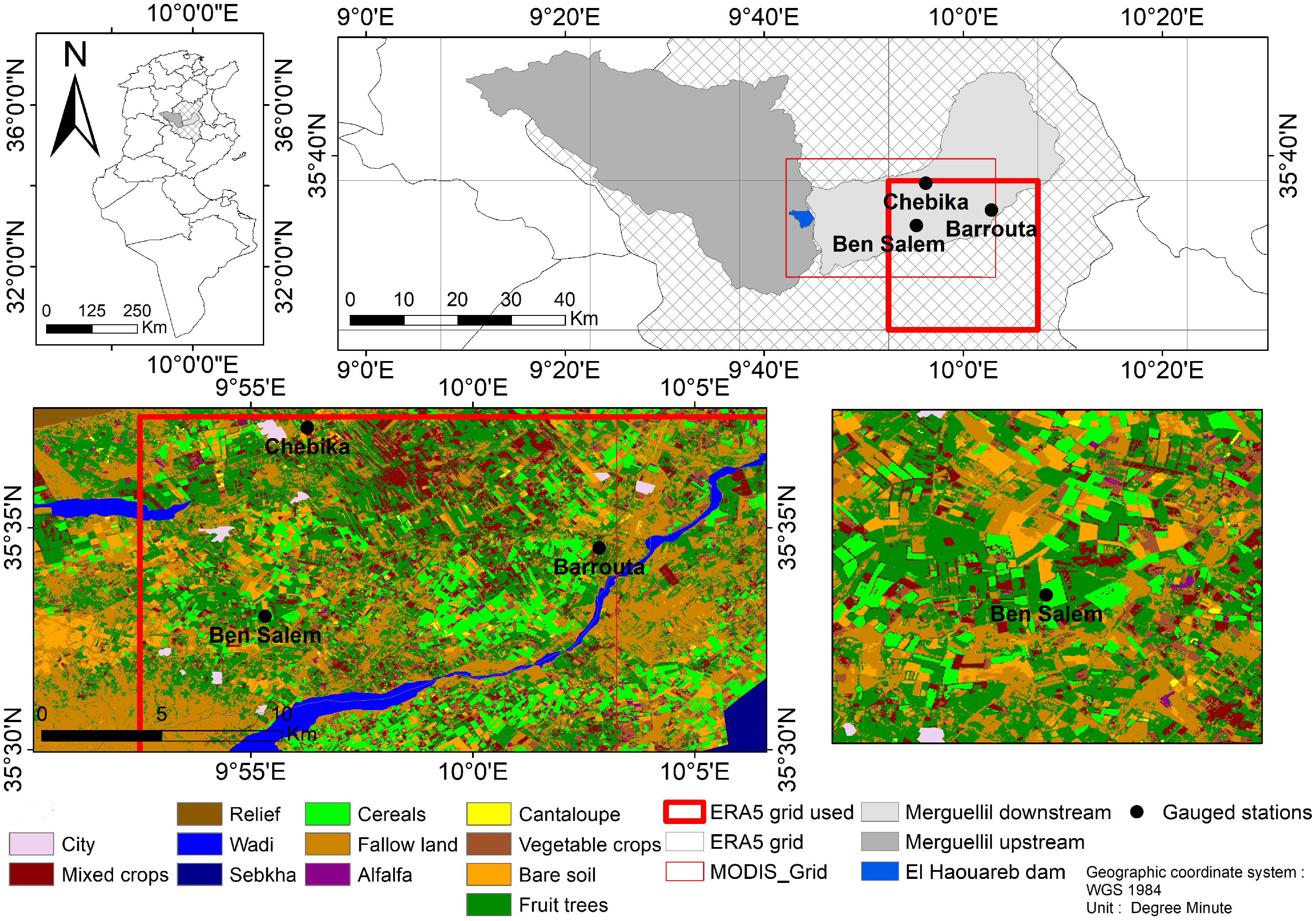
2. Study Area
3. Data and Methodology
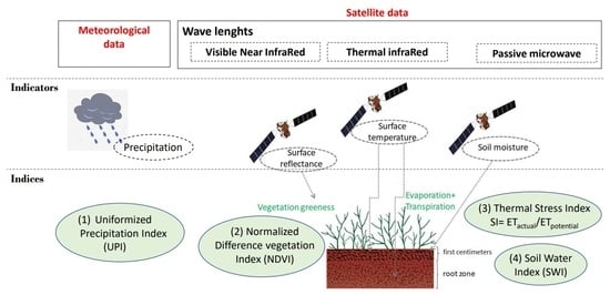
3.1. Biophysical Indices Derivation
3.1.1. NDVI
3.1.2. SWI
3.1.3. Thermal Infrared Stress Index
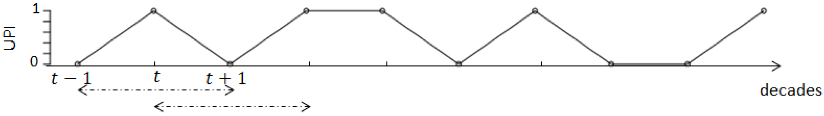
3.1.4. UPI
3.2. Thermal Stress Index Derived from Energy Balance Model
3.2.1. SPARSE Model
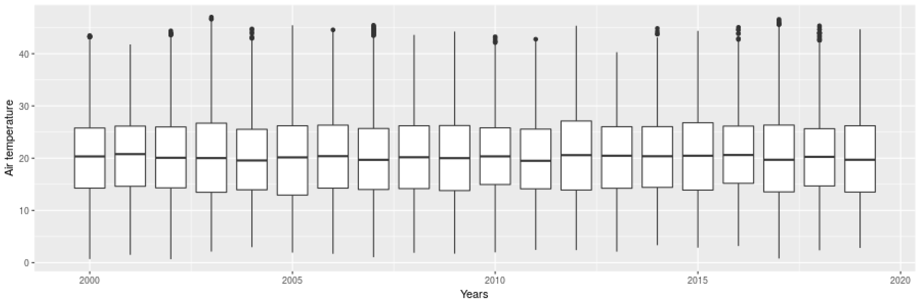
3.2.2. Meteorological Forcing
- Unprocessed reanalysis data ERA5 extracted at the grid cell closest to the region of interest (see Figure 1): ERA5 reanalyses are available at a 31 km spatial resolution [64]) from 1950 to present at an hourly temporal scale [64]. Reanalysis series that correspond to the four meteorological variables required for the energy balance model to simulate the corresponding index are: the incoming global solar radiation at the surface (bottom of atmosphere), wind speed at 10 m, air temperature at 2 m and the relative humidity that was derived from 2 m air temperature and 2 m dewpoint temperature ERA5 products, according to the procedures defined in [65]. The specific aim of using unprocessed reanalysis data for our study, is to assess its performance to constrain an energy balance model for regions with no gauged stations.
- Simulated series from a Stochastic Weather Generator (SWG) called “MetGen” [49]: Its implementation is publicly and freely available as an R library. MetGen generates scenarios of meteorological variables at sub-daily temporal resolution in order to extend local observations in the past. It relies on low resolution ERA5 reanalysis data and exploits observations provided by three gauged stations located in our study region (see Figure 1) to simulate regional climatic information. The corresponding index simulated using the SWG meteorological to constrain SPARSE model, is denoted .
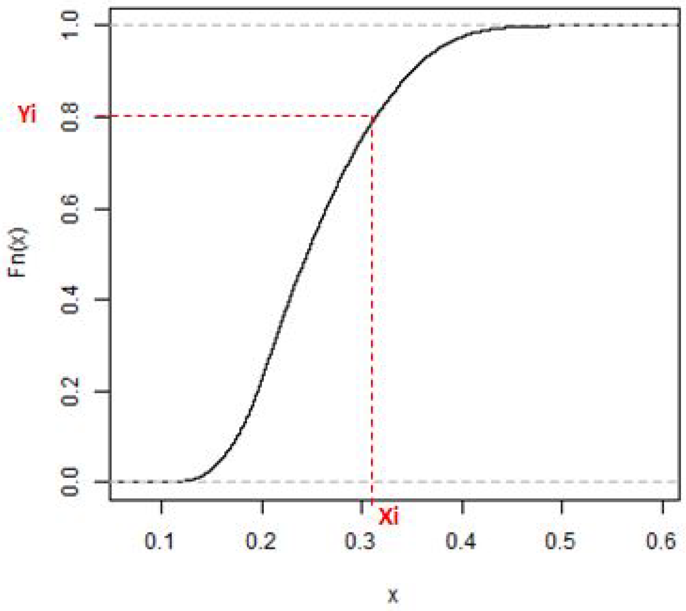
3.3. Indices Standardization
3.4. Evaluation of the Different Drought Indices Performance
3.4.1. At Regional Scale
3.4.2. At Local Scale
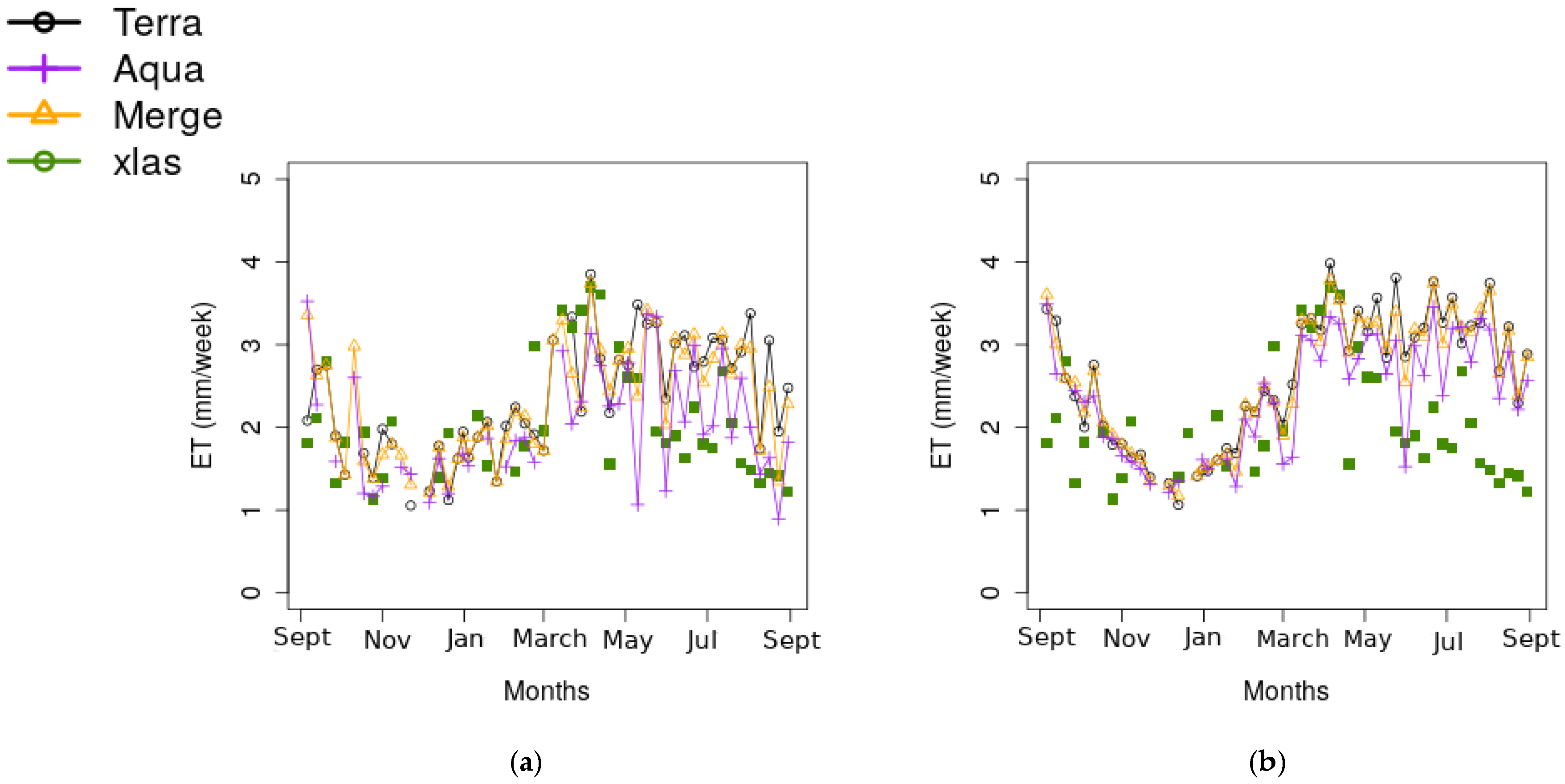
- XLAS in-situ measurements: Sensible heat flux measurements using an extra-large aperture scintillometer (XLAS) are provided as part of the work of [60], for the period ranging between March 2013 and June 2015. The scintillometer (XLAS) was installed close to the Ben Salem village over a 4 km transect above a mixed vegetation canopy: trees (mainly olive orchards) with some annual crops (cereals and market gardening) [60]. For our analyses, pixels enclosed in the mean XLAS are selected in order to compare the different drought indices with the stress index derived from the sensible heat flux measurements, denoted .
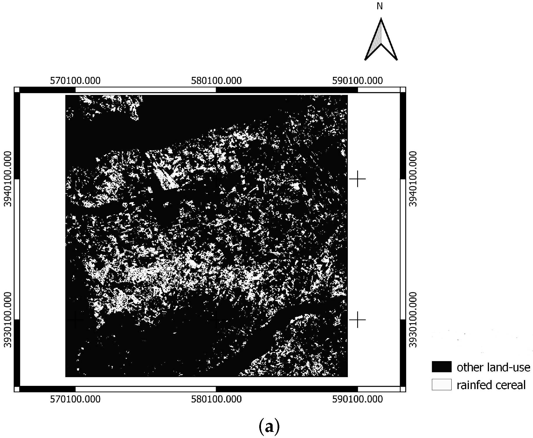
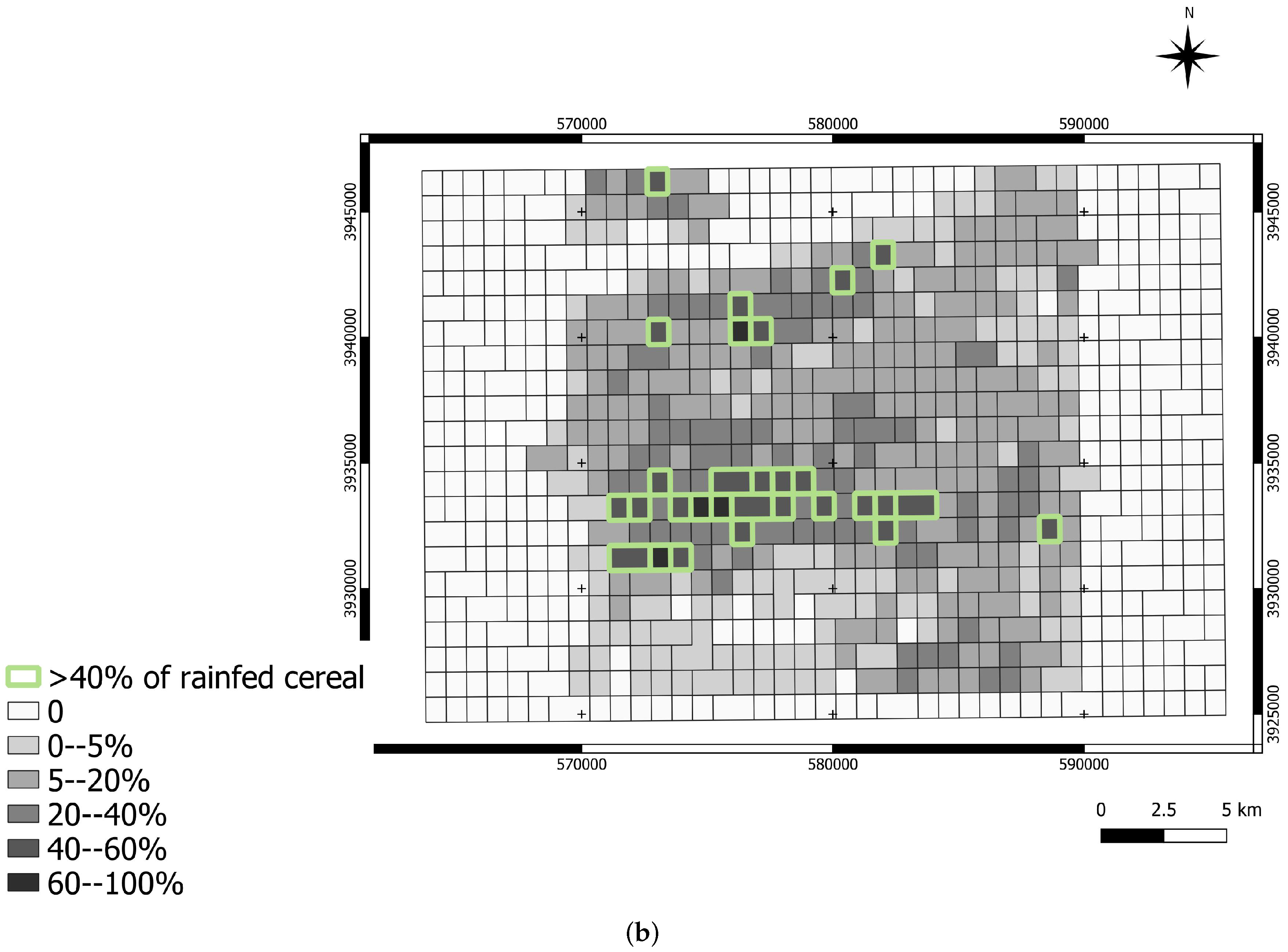
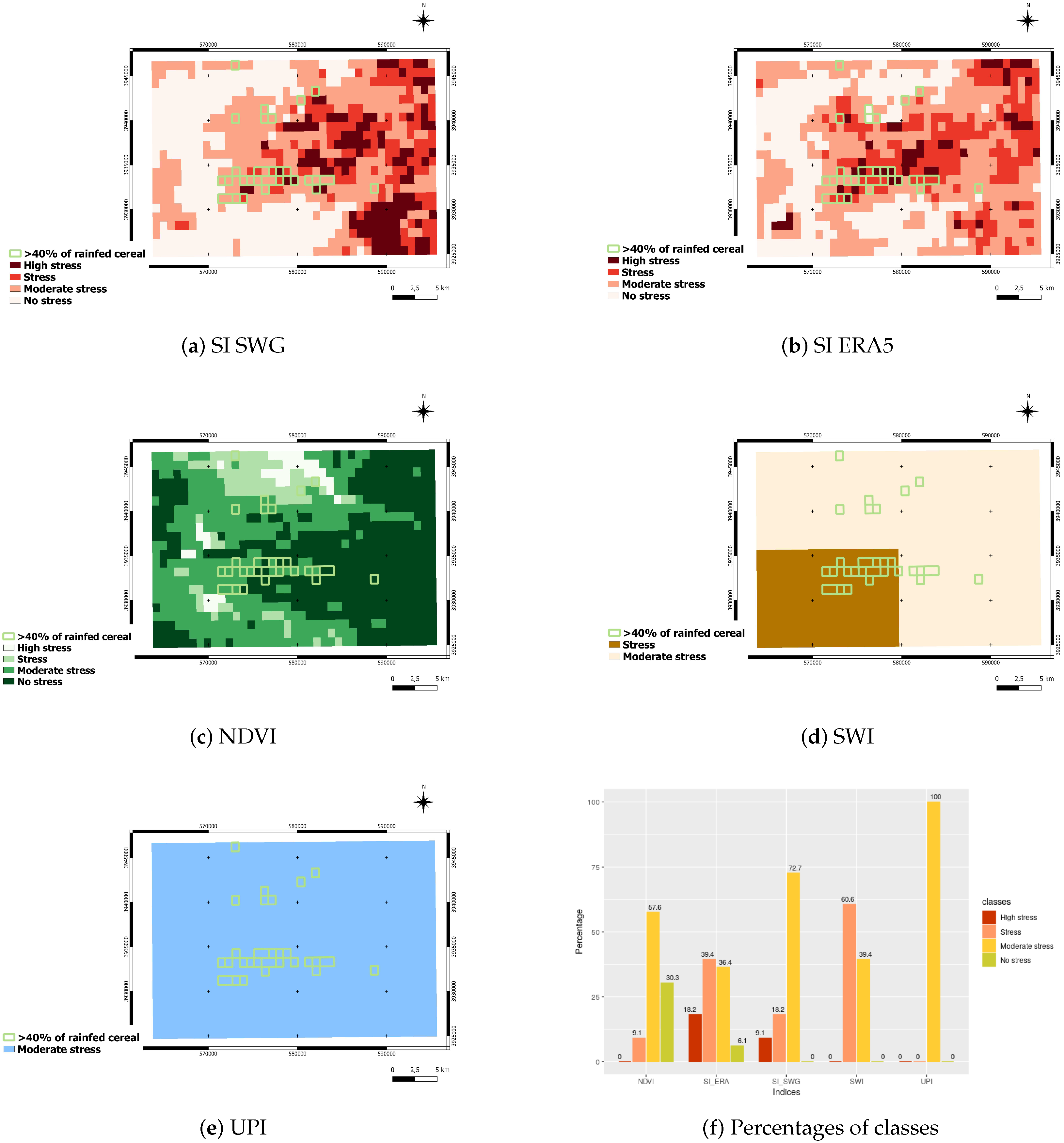
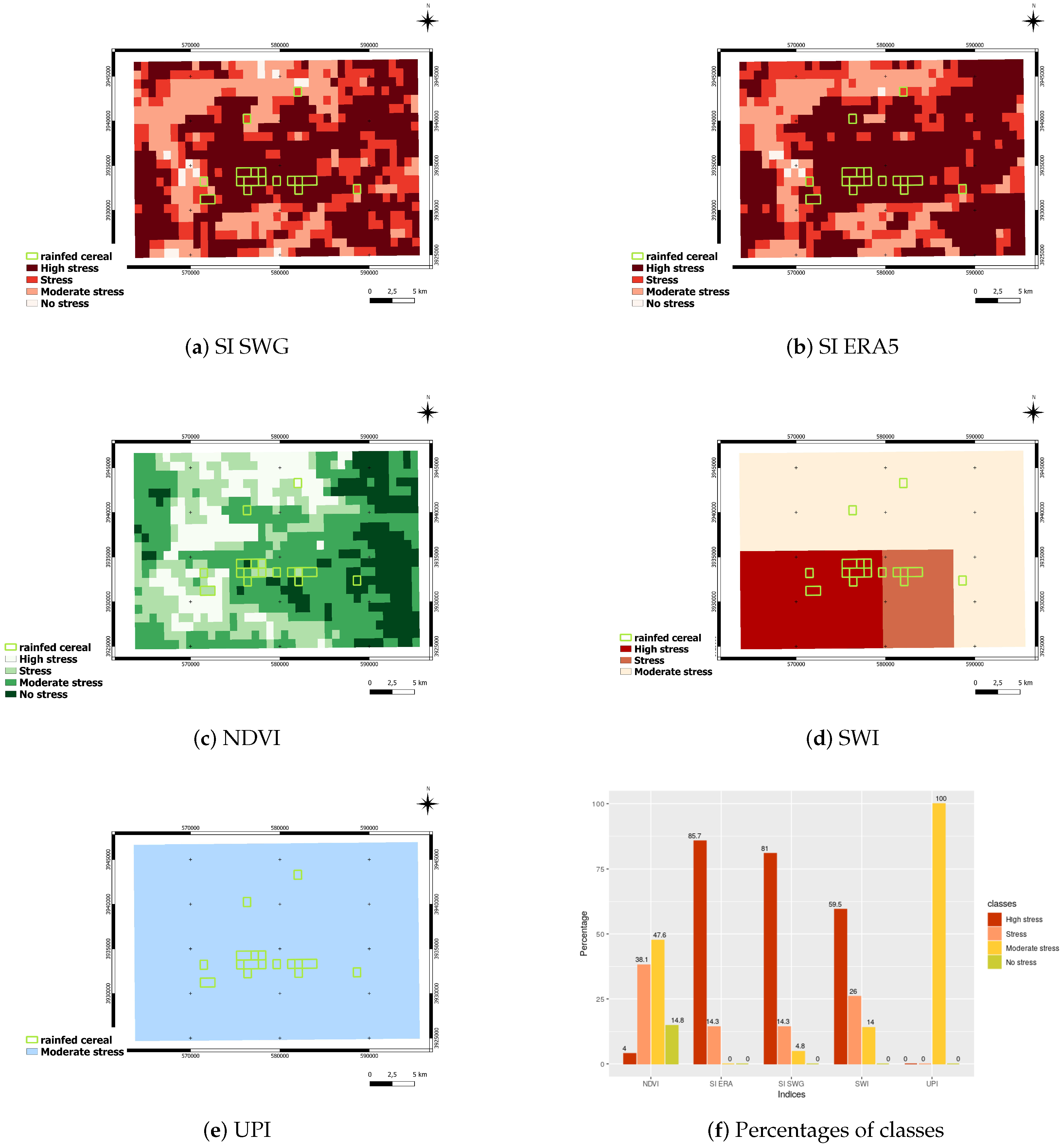
- Historical rainfed areas selection: Rainfed crops are more sensitive to rainfall depletion and thus to drought. For our analyses, we identify historical rainfed wheat areas relying on a non-irrigated cereal mask (see Figure 5a), computed for the agricultural year 2011–2012, as part of the work computed by [68]. It is computed using an object-oriented classification technique basing on the Spot image of 31 March 2012. We generate the percentage of non-irrigated cereal fields for this year, over each MODIS pixel, (see Figure 5b). Then, we select pixels that contain more than 40% of rainfed cereal cover. Rainfed cereal pixels selected are used as reference to locate non-irrigated cereal fields in precedent years, in order to assess the response of the different indices over a dry and a wet year.
4. Results
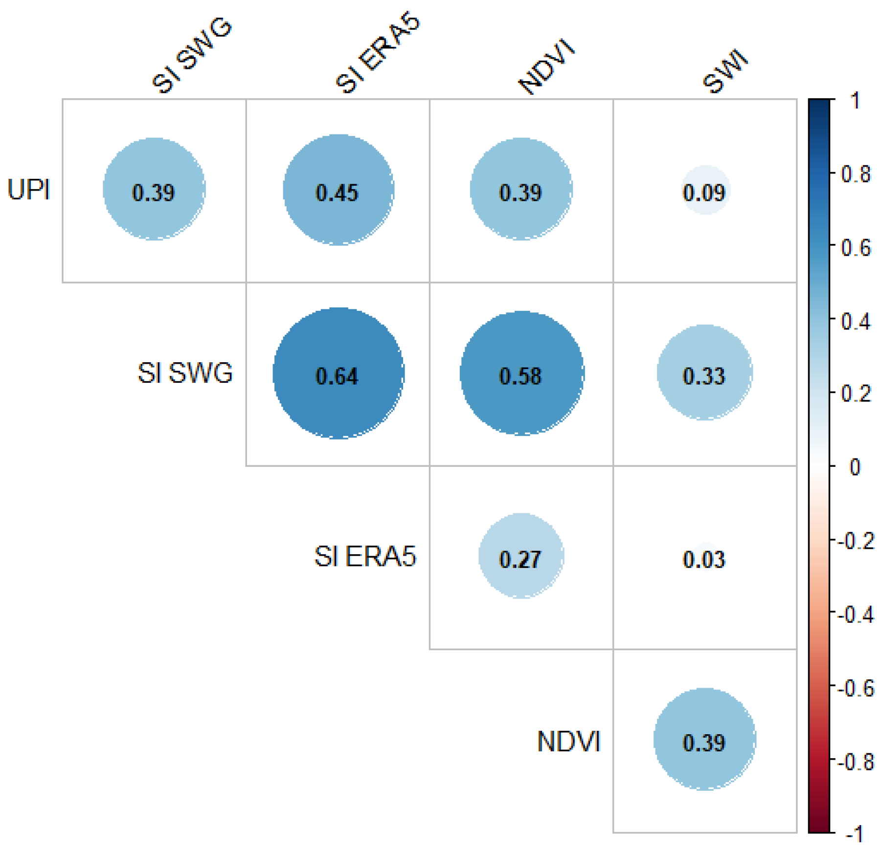
4.1. Drought Indices Inter-Comparison at Regional Scale
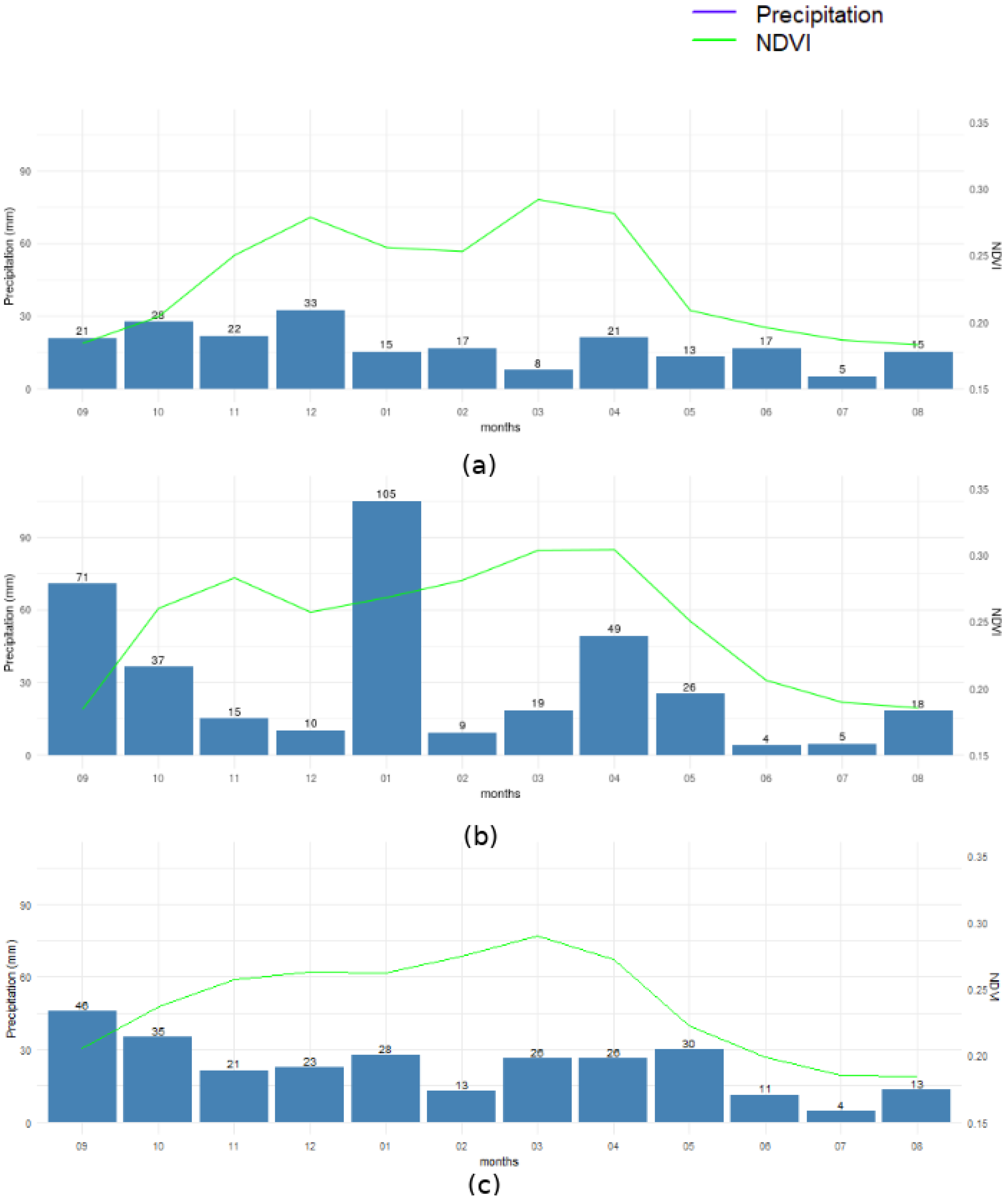
4.1.1. Annual Scale
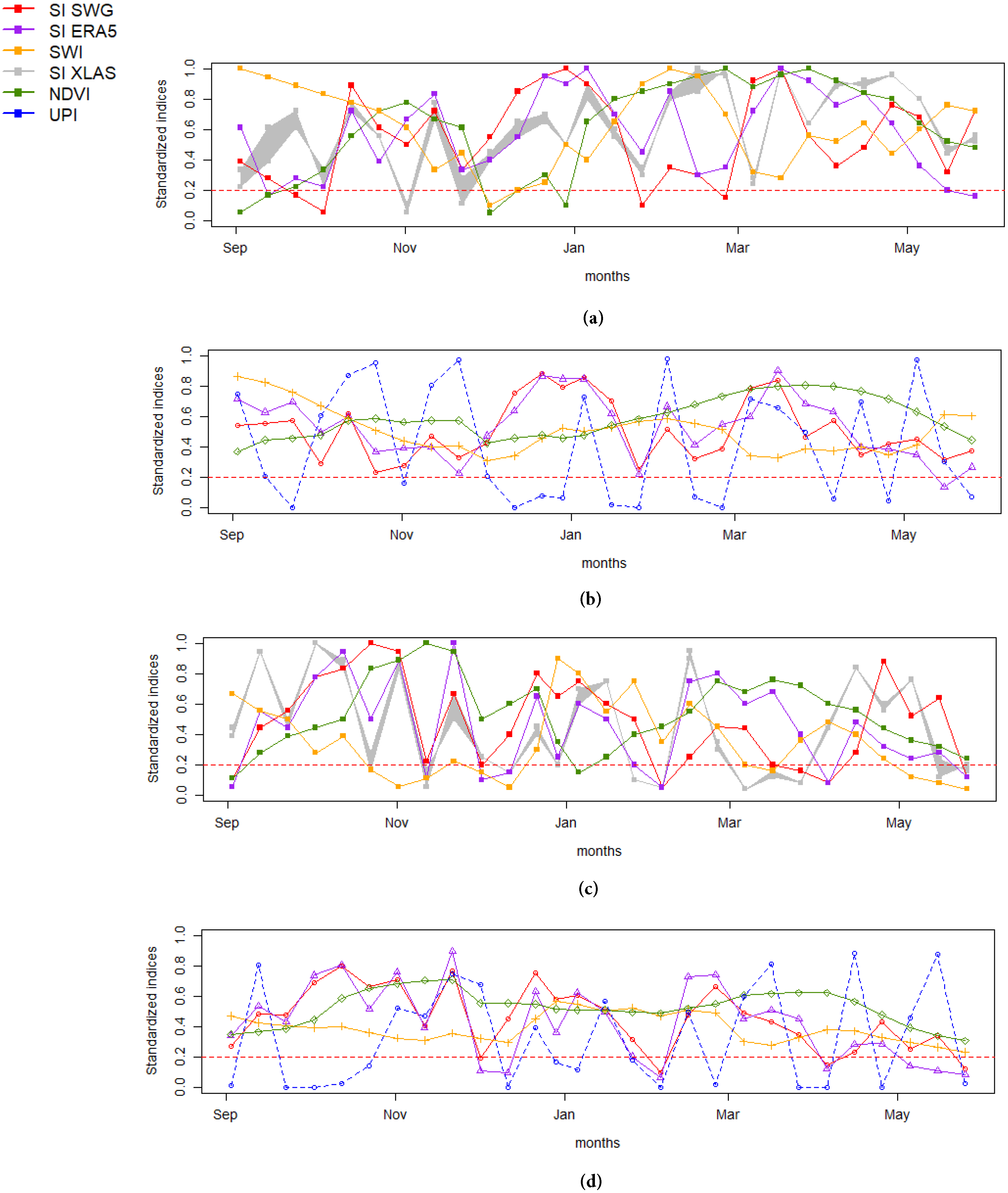
4.1.2. Decadal Scale
4.2. Drought Indices Inter-Comparison at Local Scale
4.2.1. Evaluation with XLAS In-Situ Measurements
4.2.2. Drought Detection in Rainfed Areas
5. Discussion
6. Conclusions
Author Contributions
Funding
Institutional Review Board Statement
Informed Consent Statement
Data Availability Statement
Acknowledgments
Conflicts of Interest
Appendix A. Post-Processing of Instantaneous Evapotranspiration Estimates
Appendix A.1. Extrapolation
Appendix A.2. TERRA ET and AQUA ET Merge
Appendix A.3. Interpolation
Appendix B. Daily ET Simulations

References
- Wilhite, D.A.; Svoboda, M.D. Drought early warning systems in the context of drought preparedness and mitigation. In Early Warning Systems for Drought Preparedness and Drought Management; World Meteorological Organization: Geneva, Swtizerland, 2000; pp. 1–21. [Google Scholar]
- Schilling, J.; Hertig, E.; Tramblay, Y.; Scheffran, J. Climate change vulnerability, water resources and social implications in North Africa. Reg. Environ. Chang. 2020, 20, 1–12. [Google Scholar] [CrossRef] [Green Version]
- MassonDelmotte, V.; Zhai, P.; Pirani, A.; Connors, S.L.; Péan, C.; Berger, S.; Caud, N.; Chen, Y.; Goldfarb, L.; Gomis, M.I.; et al. (Eds.) Summary for Policymakers. In Climate Change 2021: The Physical Science Basis. Contribution of Working Group I to the Sixth Assessment Report of the Intergovernmental Panel on Climate Change; Cambridge University Press: Cambridge, UK, 2021. [Google Scholar]
- Anderson, M.C.; Hain, C.; Wardlow, B.; Pimstein, A.; Mecikalski, J.R.; Kustas, W.P. Evaluation of drought indices based on thermal remote sensing of evapotranspiration over the continental United States. J. Clim. 2011, 24, 2025–2044. [Google Scholar] [CrossRef]
- Otkin, J.A.; Anderson, M.C.; Hain, C.; Mladenova, I.E.; Basara, J.B.; Svoboda, M. Examining rapid onset drought development using the thermal infrared–based evaporative stress index. J. Hydrometeorol. 2013, 14, 1057–1074. [Google Scholar] [CrossRef]
- Mishra, A.K.; Singh, V.P. A review of drought concepts. J. Hydrol. 2010, 391, 202–216. [Google Scholar] [CrossRef]
- McKee, T.B.; Doesken, N.J.; Kleist, J. The relationship of drought frequency and duration to time scales. In Proceedings of the 8th Conference on Applied Climatology, Boston, MA, USA, 17–22 January 1993; Volume 17, pp. 179–183. [Google Scholar]
- Mishra, A.; Desai, V. Drought forecasting using stochastic models. Stoch. Environ. Res. Risk Assess. 2005, 19, 326–339. [Google Scholar] [CrossRef]
- Mishra, A.; Singh, V.P. Analysis of drought severity-area-frequency curves using a general circulation model and scenario uncertainty. J. Geophys. Res. Atmos. 2009, 114, D06120. [Google Scholar] [CrossRef]
- Zhang, J.; Xu, Y.; Yao, F.; Wang, P.; Guo, W.; Li, L.; Yang, L. Advances in estimation methods of vegetation water content based on optical remote sensing techniques. Sci. China Technol. Sci. 2010, 53, 1159–1167. [Google Scholar] [CrossRef]
- AghaKouchak, A. Advancements in Satellite Remote Sensing for Drought Monitoring. In Drought and Water Crises; CRC Press: Boca Raton, FL, USA, 2017; pp. 225–258. [Google Scholar]
- Dorigo, W.; Wagner, W.; Albergel, C.; Albrecht, F.; Balsamo, G.; Brocca, L.; Chung, D.; Ertl, M.; Forkel, M.; Gruber, A.; et al. ESA CCI Soil Moisture for improved Earth system understanding: State-of-the art and future directions. Remote Sens. Environ. 2017, 203, 185–215. [Google Scholar] [CrossRef]
- Wigneron, J.P.; Chanzy, A.; Calvet, J.C.; Bruguier, N. A simple algorithm to retrieve soil moisture and vegetation biomass using passive microwave measurements over crop fields. Remote Sens. Environ. 1995, 51, 331–341. [Google Scholar] [CrossRef]
- Zribi, M.; Nativel, S.; Le Page, M. Analysis of Agronomic Drought in a Highly Anthropogenic Context Based on Satellite Monitoring of Vegetation and Soil Moisture. Remote Sens. 2021, 13, 2698. [Google Scholar] [CrossRef]
- Amri, R.; Zribi, M.; Lili-Chabaane, Z.; Wagner, W.; Hasenauer, S. Analysis of C-band scatterometer moisture estimations derived over a semiarid region. IEEE Trans. Geosci. Remote Sens. 2012, 50, 2630–2638. [Google Scholar] [CrossRef]
- Zhang, D.; Tang, R.; Zhao, W.; Tang, B.; Wu, H.; Shao, K.; Li, Z.L. Surface soil water content estimation from thermal remote sensing based on the temporal variation of land surface temperature. Remote Sens. 2014, 6, 3170–3187. [Google Scholar] [CrossRef] [Green Version]
- Jiao, W.; Wang, L.; McCabe, M.F. Multi-sensor remote sensing for drought characterization: Current status, opportunities and a roadmap for the future. Remote Sens. Environ. 2021, 256, 112313. [Google Scholar] [CrossRef]
- Tucker, C.J. Red and photographic infrared linear combinations for monitoring vegetation. Remote Sens. Environ. 1979, 8, 127–150. [Google Scholar] [CrossRef] [Green Version]
- Kogan, F.N. Application of vegetation index and brightness temperature for drought detection. Adv. Space Res. 1995, 15, 91–100. [Google Scholar] [CrossRef]
- Quiring, S.M.; Ganesh, S. Evaluating the utility of the Vegetation Condition Index (VCI) for monitoring meteorological drought in Texas. Agric. For. Meteorol. 2010, 150, 330–339. [Google Scholar] [CrossRef]
- Kogan, F.N. Operational space technology for global vegetation assessment. Bull. Am. Meteorol. Soc. 2001, 82, 1949–1964. [Google Scholar] [CrossRef]
- Amri, R.; Zribi, M.; Lili-Chabaane, Z.; Duchemin, B.; Gruhier, C.; Chehbouni, A. Analysis of vegetation behavior in a North African semi-arid region, using SPOT-VEGETATION NDVI data. Remote Sens. 2011, 3, 2568–2590. [Google Scholar] [CrossRef] [Green Version]
- Farrar, T.; Nicholson, S.; Lare, A. The influence of soil type on the relationships between NDVI, rainfall, and soil moisture in semiarid Botswana. II. NDVI response to soil oisture. Remote Sens. Environ. 1994, 50, 121–133. [Google Scholar] [CrossRef]
- Ozelkan, E.; Chen, G.; Ustundag, B.B. Multiscale object-based drought monitoring and comparison in rainfed and irrigated agriculture from Landsat 8 OLI imagery. Int. J. Appl. Earth Obs. Geoinf. 2016, 44, 159–170. [Google Scholar] [CrossRef]
- AghaKouchak, A.; Farahmand, A.; Melton, F.; Teixeira, J.; Anderson, M.; Wardlow, B.D.; Hain, C. Remote sensing of drought: Progress, challenges and opportunities. Rev. Geophys. 2015, 53, 452–480. [Google Scholar] [CrossRef] [Green Version]
- Paulik, C.; Dorigo, W.; Wagner, W.; Kidd, R. Validation of the ASCAT Soil Water Index using in situ data from the International Soil Moisture Network. Int. J. Appl. Earth Obs. Geoinf. 2014, 30, 1–8. [Google Scholar] [CrossRef]
- Paulik, C.; Naeimi, V.; Dorigo, W.; Wagner, W.; Kidd, R. A global validation of the ASCAT Soil Water Index (SWI) with in situ data from the International Soil Moisture Network. In Proceedings of the EGU General Assembly Conference Abstracts, Vienna, Austria, 22–27 April 2012; p. 10189. [Google Scholar]
- Baghdadi, N.; Cresson, R.; El Hajj, M.; Ludwig, R.; La Jeunesse, I. Soil parameters estimation over bare agriculture areas from C-band polarimetric SAR data using neural networks. Hydrol. Earth Syst. Sci. Discuss. 2012, 9, 2897–2933. [Google Scholar] [CrossRef] [Green Version]
- Babaeian, E.; Sadeghi, M.; Jones, S.B.; Montzka, C.; Vereecken, H.; Tuller, M. Ground, proximal, and satellite remote sensing of soil moisture. Rev. Geophys. 2019, 57, 530–616. [Google Scholar] [CrossRef] [Green Version]
- Narasimhan, B.; Srinivasan, R. Development and evaluation of Soil Moisture Deficit Index (SMDI) and Evapotranspiration Deficit Index (ETDI) for agricultural drought monitoring. Agric. For. Meteorol. 2005, 133, 69–88. [Google Scholar] [CrossRef]
- Zhang, N.; Hong, Y.; Qin, Q.; Liu, L. VSDI: A visible and shortwave infrared drought index for monitoring soil and vegetation moisture based on optical remote sensing. Int. J. Remote Sens. 2013, 34, 4585–4609. [Google Scholar] [CrossRef]
- Jackson, R.D.; Idso, S.; Reginato, R.; Pinter, P., Jr. Canopy temperature as a crop water stress indicator. Water Resour. Res. 1981, 17, 1133–1138. [Google Scholar] [CrossRef]
- Wang, X.; Zhao, C.; Guo, N.; Li, Y.; Jian, S.; Yu, K. Determining the canopy water stress for spring wheat using canopy hyperspectral reflectance data in loess plateau semiarid regions. Spectrosc. Lett. 2015, 48, 492–498. [Google Scholar] [CrossRef]
- Jones, H.G.; Serraj, R.; Loveys, B.R.; Xiong, L.; Wheaton, A.; Price, A.H. Thermal infrared imaging of crop canopies for the remote diagnosis and quantification of plant responses to water stress in the field. Funct. Plant Biol. 2009, 36, 978–989. [Google Scholar] [CrossRef] [Green Version]
- Anderson, M.C.; Zolin, C.A.; Sentelhas, P.C.; Hain, C.R.; Semmens, K.; Yilmaz, M.T.; Gao, F.; Otkin, J.A.; Tetrault, R. The Evaporative Stress Index as an indicator of agricultural drought in Brazil: An assessment based on crop yield impacts. Remote Sens. Environ. 2016, 174, 82–99. [Google Scholar] [CrossRef]
- Norman, J.M.; Kustas, W.P.; Humes, K.S. Source approach for estimating soil and vegetation energy fluxes in observations of directional radiometric surface temperature. Agric. For. Meteorol. 1995, 77, 263–293. [Google Scholar] [CrossRef]
- Lili, Z.; Duchesne, J.; Nicolas, H.; Rivoal, R.; de Breger, P. Détection infrarouge thermique des maladies du blé d’hiver 1. Eppo Bull. 1991, 21, 659–672. [Google Scholar] [CrossRef]
- Sheffield, J.; Wood, E.F. Drought: Past Problems and Future Scenarios; Routledge: London, UK, 2012. [Google Scholar]
- Lagouarde, J.P.; Boulet, G. Energy balance of continental surfaces and the use of surface temperature. In Land Surface Remote Sensing in Continental Hydrology; Elsevier: Amsterdam, The Netherlands, 2016; pp. 323–361. [Google Scholar]
- Boulet, G.; Chehbouni, A.; Gentine, P.; Duchemin, B.; Ezzahar, J.; Hadria, R. Monitoring water stress using time series of observed to unstressed surface temperature difference. Agric. For. Meteorol. 2007, 146, 159–172. [Google Scholar] [CrossRef] [Green Version]
- Delogu, E.; Olioso, A.; Alliès, A.; Demarty, J.; Boulet, G. Evaluation of Multiple Methods for the Production of Continuous Evapotranspiration Estimates from TIR Remote Sensing. Remote Sens. 2021, 13, 1086. [Google Scholar] [CrossRef]
- Diarra, A.; Jarlan, L.; Er-Raki, S.; Le Page, M.; Aouade, G.; Tavernier, A.; Boulet, G.; Ezzahar, J.; Merlin, O.; Khabba, S. Performance of the two-source energy budget (TSEB) model for the monitoring of evapotranspiration over irrigated annual crops in North Africa. Agric. Water Manag. 2017, 193, 71–88. [Google Scholar] [CrossRef]
- Moran, M.S. Thermal infrared measurement as an indicator of plant ecosystem health. In Thermal Remote Sensing in Land Surface Processes; CRC Press: Boca Raton, FL, USA, 2004; pp. 256–282. [Google Scholar]
- Moran, M.; Clarke, T.; Inoue, Y.; Vidal, A. Estimating crop water deficit using the relation between surface-air temperature and spectral vegetation index. Remote Sens. Environ. 1994, 49, 246–263. [Google Scholar] [CrossRef]
- Cunha, A.P.; Zeri, M.; Deusdará Leal, K.; Costa, L.; Cuartas, L.A.; Marengo, J.A.; Tomasella, J.; Vieira, R.M.; Barbosa, A.A.; Cunningham, C.; et al. Extreme drought events over Brazil from 2011 to 2019. Atmosphere 2019, 10, 642. [Google Scholar] [CrossRef] [Green Version]
- Cunha, A.; Alvalá, R.C.; Nobre, C.A.; Carvalho, M.A. Monitoring vegetative drought dynamics in the Brazilian semiarid region. Agric. For. Meteorol. 2015, 214, 494–505. [Google Scholar] [CrossRef]
- Abbas, S.; Nichol, J.E.; Qamer, F.M.; Xu, J. Characterization of drought development through remote sensing: A case study in Central Yunnan, China. Remote Sens. 2014, 6, 4998–5018. [Google Scholar] [CrossRef] [Green Version]
- Chirouze, J.; Boulet, G.; Jarlan, L.; Fieuzal, R.; Rodriguez, J.; Ezzahar, J.; Raki, S.E.; Bigeard, G.; Merlin, O.; Garatuza-Payan, J.; et al. Intercomparison of four remote-sensing-based energy balance methods to retrieve surface evapotranspiration and water stress of irrigated fields in semi-arid climate. Hydrol. Earth Syst. Sci. Discuss. 2014, 18, 1165–1188. [Google Scholar] [CrossRef] [Green Version]
- Farhani, N.; Carreau, J.; Boulet, G.; Kassouk, Z.; Mougenot, B.; Le Page, M.; Lili Chabaane, Z.; Zitouna, R. Scenarios of hydrometeorological variables based on auxiliary data for water stress retrieval in central Tunisia. In Proceedings of the 2020 Mediterranean and Middle-East Geoscience and Remote Sensing Symposium (M2GARSS), Tunis, Tunisia, 9–11 March 2020; pp. 293–296. [Google Scholar]
- Boulet, G.; Mougenot, B.; Lhomme, J.; Fanise, P.; Lili-Chabaane, Z.; Olioso, A.; Bahir, M.; Rivalland, V.; Jarlan, L.; Merlin, O.; et al. The SPARSE model for the prediction of water stress and evapotranspiration components from thermal infra-red data and its evaluation over irrigated and rainfed wheat. Hydrol. Earth Syst. Sci. Discuss. 2015, 19, 4653–4672. [Google Scholar] [CrossRef] [Green Version]
- Alazard, M.; Leduc, C.; Travi, Y.; Boulet, G.; Salem, A.B. Estimating evaporation in semi-arid areas facing data scarcity: Example of the El Haouareb dam (Merguellil catchment, Central Tunisia). J. Hydrol. Reg. Stud. 2015, 3, 265–284. [Google Scholar] [CrossRef] [Green Version]
- Massuel, S.; Riaux, J. Groundwater overexploitation: Why is the red flag waved? Case study on the Kairouan plain aquifer (central Tunisia). Hydrogeol. J. 2017, 25, 1607–1620. [Google Scholar] [CrossRef]
- Leduc, C.; Ammar, S.B.; Favreau, G.; Beji, R.; Virrion, R.; Lacombe, G.; Tarhouni, J.; Aouadi, C.; Chelli, B.; Jebnoun, N.; et al. Impacts of hydrological changes in the Mediterranean zone: Environmental modifications and rural development in the Merguellil catchment, central Tunisia/ Un exemple d’évolution hydrologique en Méditerranée: Impacts des modifications environnementales et du développement agricole dans le bassin-versant du Merguellil (Tunisie centrale). Hydrol. Sci. J./J. des Sci. Hydrol. 2007, 52, 1162–1178. [Google Scholar]
- Molle, F.; Wester, P. River Basin Trajectories: Societies, Environments and Development; IWMI: Oxford, UK, 2009; Volume 8. [Google Scholar]
- Ceballos, A.; Scipal, K.; Wagner, W.; Martínez-Fernández, J. Validation of ERS scatterometer-derived soil moisture data in the central part of the Duero Basin, Spain. Hydrol. Process. Int. J. 2005, 19, 1549–1566. [Google Scholar] [CrossRef]
- Kanzari, S.; Hachicha, M.; Bouhlila, R.; Battle-Sales, J. Characterization and modeling of water movement and salts transfer in a semi-arid region of Tunisia (Bou Hajla, Kairouan)–Salinization risk of soils and aquifers. Comput. Electron. Agric. 2012, 86, 34–42. [Google Scholar] [CrossRef]
- Brocca, L.; Ciabatta, L.; Moramarco, T.; Ponziani, F.; Berni, N.; Wagner, W. Use of satellite soil moisture products for the operational mitigation of landslides risk in central Italy. In Satellite Soil Moisture Retrieval; Elsevier: Amsterdam, The Netherlands, 2016; pp. 231–247. [Google Scholar]
- Paulik, C. Copernicus Global Land Operations “Vegetation and Energy”; TU Wien: Vienna, Austria, 2017. [Google Scholar]
- Clevers, J. Application of a weighted infrared-red vegetation index for estimating leaf area index by correcting for soil moisture. Remote Sens. Environ. 1989, 29, 25–37. [Google Scholar] [CrossRef]
- Saadi, S.; Boulet, G.; Bahir, M.; Brut, A.; Delogu, E.; Fanise, P.; Mougenot, B.; Simonneaux, V.; Lili Chabaane, Z. Assessment of actual evapotranspiration over a semi arid heterogeneous land surface by means of coupled low-resolution remote sensing data with an energy balance model: Comparison to extra-large aperture scintillometer measurements. Hydrol. Earth Syst. Sci. 2018, 22, 2187–2209. [Google Scholar] [CrossRef] [Green Version]
- Funk, C.; Peterson, P.; Landsfeld, M.; Pedreros, D.; Verdin, J.; Shukla, S.; Husak, G.; Rowland, J.; Harrison, L.; Hoell, A.; et al. The climate hazards infrared precipitation with stations—A new environmental record for monitoring extremes. Sci. Data 2015, 2, 1–21. [Google Scholar] [CrossRef] [Green Version]
- Bouaziz, M.; Medhioub, E.; Csaplovisc, E. A machine learning model for drought tracking and forecasting using remote precipitation data and a standardized precipitation index from arid regions. J. Arid. Environ. 2021, 189, 104478. [Google Scholar] [CrossRef]
- Massman, W. A surface energy balance method for partitioning evapotranspiration data into plant and soil components for a surface with partial canopy cover. Water Resour. Res. 1992, 28, 1723–1732. [Google Scholar] [CrossRef]
- Hersbach, H.; Bell, B.; Berrisford, P.; Hirahara, S.; Horányi, A.; Muñoz-Sabater, J.; Nicolas, J.; Peubey, C.; Radu, R.; Schepers, D.; et al. The ERA5 global reanalysis. Q. J. R. Meteorol. Soc. 2020, 146, 1999–2049. [Google Scholar] [CrossRef]
- Allen, R.G.; Pereira, L.S.; Raes, D.; Smith, M. Crop evapotranspiration-Guidelines for computing crop water requirements-FAO Irrigation and drainage paper 56. Fao Rome 1998, 300, D05109. [Google Scholar]
- Mega, N.; Medjerab, A. Statistical comparison between the standardized precipitation index and the standardized precipitation drought index. Model. Earth Syst. Environ. 2021, 7, 373–388. [Google Scholar] [CrossRef]
- Hoffman, R.N.; Boukabara, S.A.; Kumar, V.K.; Garrett, K.; Casey, S.P.; Atlas, R. An empirical cumulative density function approach to defining summary NWP forecast assessment metrics. Mon. Weather Rev. 2017, 145, 1427–1435. [Google Scholar] [CrossRef]
- Chahbi Bellakanji, A.; Zribi, M.; Lili-Chabaane, Z.; Mougenot, B. Forecasting of cereal yields in a semi-arid area using the simple algorithm for yield estimation (SAFY) agro-meteorological model combined with optical SPOT/HRV images. Sensors 2018, 18, 2138. [Google Scholar] [CrossRef] [Green Version]
- Joe, H. Multivariate Models and Multivariate Dependence Concepts; CRC Press: Boca Raton, FL, USA, 1997. [Google Scholar]
- Delogu, E.; Boulet, G.; Olioso, A.; Coudert, B.; Chirouze, J.; Ceschia, E.; Le Dantec, V.; Marloie, O.; Chehbouni, G.; Lagouarde, J.P. Reconstruction of temporal variations of evapotranspiration using instantaneous estimates at the time of satellite overpass. Hydrol. Earth Syst. Sci. 2012, 16, 2995–3010. [Google Scholar] [CrossRef] [Green Version]
- Lhomme, J.P.; Elguero, E. Examination of evaporative fraction diurnal behaviour using a soil-vegetation model coupled with a mixed-layer model. Hydrol. Earth Syst. Sci. 1999, 3, 259–270. [Google Scholar] [CrossRef]
- Hoedjes, J.; Chehbouni, A.; Jacob, F.; Ezzahar, J.; Boulet, G. Deriving daily evapotranspiration from remotely sensed instantaneous evaporative fraction over olive orchard in semi-arid Morocco. J. Hydrol. 2008, 354, 53–64. [Google Scholar] [CrossRef] [Green Version]
- Jackson, R.D.; Hatfield, J.L.; Reginato, R.; Idso, S.; Pinter, P., Jr. Estimation of daily evapotranspiration from one time-of-day measurements. Agric. Water Manag. 1983, 7, 351–362. [Google Scholar] [CrossRef]
- Michelangeli, P.A.; Vrac, M.; Loukos, H. Probabilistic downscaling approaches: Application to wind cumulative distribution functions. Geophys. Res. Lett. 2009, 36, L11708. [Google Scholar] [CrossRef]


| Wave Lenghts | Visible/Near Infrared | Infrared + Visible + Meteo. | Microwave | Meteo. + Satellites Data | |
|---|---|---|---|---|---|
| Indices | NDVI | SWI | UPI | ||
| Satellites | MODIS | MODIS | MODIS | ASCAT | CHIRPS |
| Model used | ✗ | SPARSE | SPARSE | ✗ | ✗ |
| Spatial resolution | 1 km | 1 km | 1 km | 12.5 km | 5 km |
| Temporal resolution | daily | daily | daily | daily | daily |
| Temporal availability | since 2000 | since 2000 | since 2000 | since 2007 | since 1981 |
| Index Values | Drought Class |
|---|---|
| 0–0.15 | High stress |
| 0.15–0.3 | Stress |
| 0.3–0.7 | Moderate stress |
| 0.7–1 | No stress |
Publisher’s Note: MDPI stays neutral with regard to jurisdictional claims in published maps and institutional affiliations. |
© 2022 by the authors. Licensee MDPI, Basel, Switzerland. This article is an open access article distributed under the terms and conditions of the Creative Commons Attribution (CC BY) license (https://creativecommons.org/licenses/by/4.0/).
Share and Cite
Farhani, N.; Carreau, J.; Kassouk, Z.; Le Page, M.; Lili Chabaane, Z.; Boulet, G. Analysis of Multispectral Drought Indices in Central Tunisia. Remote Sens. 2022, 14, 1813. https://doi.org/10.3390/rs14081813
Farhani N, Carreau J, Kassouk Z, Le Page M, Lili Chabaane Z, Boulet G. Analysis of Multispectral Drought Indices in Central Tunisia. Remote Sensing. 2022; 14(8):1813. https://doi.org/10.3390/rs14081813
Chicago/Turabian StyleFarhani, Nesrine, Julie Carreau, Zeineb Kassouk, Michel Le Page, Zohra Lili Chabaane, and Gilles Boulet. 2022. "Analysis of Multispectral Drought Indices in Central Tunisia" Remote Sensing 14, no. 8: 1813. https://doi.org/10.3390/rs14081813